Packing multiway cuts in capacitated graphs

Abstract

We consider the following “multiway cut packing” problem in undirected graphs: we are given a graph $G=(V,E)$ and $k$ commodities, each corresponding to a set of terminals located at different vertices in the graph; our goal is to produce a collection of cuts $\{E_{1},\cdots,E_{k}\}$ such that $E_{i}$ is a multiway cut for commodity $i$ and the maximum load on any edge is minimized. The load on an edge is defined to be the number of cuts in the solution crossing the edge. In the capacitated version of the problem edges have capacities $c_{e}$ and the goal is to minimize the maximum relative load on any edge – the ratio of the edge’s load to its capacity. We present the first constant factor approximations for this problem in arbitrary undirected graphs. The multiway cut packing problem arises in the context of graph labeling problems where we are given a partial labeling of a set of items and a neighborhood structure over them, and, informally stated, the goal is to complete the labeling in the most consistent way. This problem was introduced by Rabani, Schulman, and Swamy (SODA’08), who developed an $O(\log n/\log\log n)$ approximation for it in general graphs, as well as an improved $O(\log^{2}k)$ approximation in trees. Here $n$ is the number of nodes in the graph.

We present an LP-based algorithm for the multiway cut packing problem in general graphs that guarantees a maximum edge load of at most $8{\textrm{OPT}}+4$. Our rounding approach is based on the observation that every instance of the problem admits a laminar solution (that is, no pair of cuts in the solution crosses) that is near-optimal. For the special case where each commodity has only two terminals and all commodities share a common sink (the “common sink $s$-$t$ cut packing” problem) we guarantee a maximum load of ${\textrm{OPT}}+2$. Both of these variants are NP-hard; for the common-sink case our result is nearly optimal.

1 Introduction

We study the multiway cut packing problem (MCP) introduced by Rabani, Schulman and Swamy [9]. In this problem, we are given $k$ instances of the multiway cut problem in a common graph, each instance being a set of terminals at different locations in the graph. Informally, our goal is to compute nearly-disjoint multiway cuts for each of the instances. More precisely, we aim to minimize the maximum number of cuts that any single edge in the graph belongs to. In the weighted version of this problem, different edges have different capacities; the goal is to minimize the maximum relative load of any edge, where the relative load of an edge is the ratio of the number of cuts it belongs to and its capacity.

The multiway cut packing problem belongs to the following class of graph labeling problems. We are given a partially labeled set of $n$ items along with a weighted graph over them that encodes similarity information among them. An item’s label is a string of length $k$ where each coordinate of the string is either drawn from an alphabet $\Sigma$, or is undetermined. Roughly speaking, the goal is to complete the partial labeling in the most consistent possible way. Note that completing a single specific entry (coordinate) of each item label is like finding what we call a “set multiway cut”—for $\sigma\in\Sigma$ let $S^{i}_{\sigma}$ denote the set of nodes for which the $i$th coordinate is labeled $\sigma$ in the partial labeling, then a complete and consistent labeling for this coordinate is a partition of the items into $|\Sigma|$ parts such that the $\sigma^{\text{th}}$ part contains the entire set $S^{i}_{\sigma}$. The cost of the labeling for a single pair of neighboring items in the graph is measured by the Hamming distance between the labels assigned to them. The overall cost of the labeling can then be formalized as a certain norm of the vector of (weighted) edge costs.

Different choices of norms for the overall cost give rise to different objectives. Minimizing the $\ell_{1}$ norm, for example, is the same as minimizing the sum of the edge costs. This problem decomposes into finding $k$ minimum set multiway cuts. Each set multiway cut instance can be reduced to a minimum multiway cut instance by simply merging all the items in the same set $S_{\sigma}$ into a single node in the graph, and can therefore be approximated to within a factor of $1.5$ [1]. On the other hand, minimizing the $\ell_{\infty}$ norm of edge costs (equivalently, the maximum edge cost) becomes the set multiway cut packing problem. Formally, in this problem, we are given $k$ set multiway cut instances $S^{1},\cdots,S^{k}$, where each $S^{i}=S^{i}_{1}\times S^{i}_{2}\times\cdots\times S^{i}_{|\Sigma|}$. The goal is to find $k$ cuts, with the $i$th cut separating every pair of terminals that belong to sets $S^{i}_{j_{1}}$ and $S^{i}_{j_{2}}$ with $j_{1}\neq j_{2}$, such that the maximum (weighted) cost of any edge is minimized. When $|S^{i}_{j}|=1$ for all $i\in[k]$ and $j\in\Sigma$, this is the multiway cut packing problem.

To our knowledge Rabani et al. [9] were the first to consider the multiway cut packing problem and provide approximation algorithms for it. They used a linear programming relaxation of the problem along with randomized rounding to obtain an $O(\frac{\log n}{\log\log n})$ approximation, where $n$ is the number of nodes in the given graph. This approximation ratio arises from an application of the Chernoff bounds to the randomized rounding process, and improves to an $O(1)$ factor when the optimal load is $\Omega(\log n)$. When the underlying graph is a tree, Rabani et al. use a more careful deterministic rounding technique to obtain an improved $O(\log^{2}k)$ approximation. The latter approximation factor holds also for a more general multicut packing problem (described in more detail below). One nice property of the latter approximation is that it is independent of the size of the graph, and remains small as the graph grows but $k$ remains fixed. Then, a natural open problem related to their work is whether a similar approximation guarantee independent of $n$ can be obtained even for general graphs.

Our results & techniques. We answer this question in the positive. We employ the same linear programming relaxation for this problem as Rabani et al., but develop a very different rounding algorithm. In order to produce a good integral solution our rounding algorithm requires a fractional collection of cuts that is not only feasible for the linear program but also satisfies an additional good property—the cut collection is laminar. In other words, when interpreted appropriately as subsets of nodes, no two cuts in the collection “cross” each other. Given such an input the rounding process only incurs a small additive loss in performance—the final (absolute) load on any edge is at most $3$ more than the load on that edge of the fractional solution that we started out with. Of course the laminarity condition comes at a cost – not every fractional solution to the cut packing LP can be interpreted as a laminar collection of cuts (see, e.g., Figure 9). We show that for the multiway cut problem any fractional collection of cuts can be converted into a laminar one while losing only a multiplicative factor of $8$ and an additive $o(1)$ amount in edge loads. Therefore, for every edge $e$ we obtain a final edge load of $8{\ell_{e}^{{\textrm{OPT}}}}+4$, where ${\ell_{e}^{{\textrm{OPT}}}}$ is the optimal load on the edge. We only load edges with $c_{e}\geq 1$ and since the optimal cost is at least $1$ our algorithm also obtains a purely multiplicative $12$ approximation.

Our laminarity based approach proves even more powerful in the special case of common-sink $s$-$t$ cut packing problem or CSCP. In this special case every multiway cut instance has only two terminals and all the instances share a common sink $t$. We use these properties to improve both the rounding and laminarity transformation algorithms, and ensure a final load of at most ${\ell_{e}^{{\textrm{OPT}}}}+1$ for every edge $e$. The CSCP is NP-hard (see Section 5) and so our guarantee for this special case is the best possible.

In converting a fractional laminar solution to an integral one we use an iterative rounding approach, assigning an integral cut at each iteration to an appropriate “innermost” terminal. Throughout the algorithm we maintain a partial integral cut collection and a partial fractional one and ensure that these collections together are feasible for the given multiway cut instances. As we round cuts, we “shift” or modify other fractional cuts so as to maintain bounds on edge loads. Maintaining feasibility and edge loads simultaneously turns out to be relatively straightforward in the case of common-sink $s$-$t$ cut packing – we only need to ensure that none of the cuts in the fractional or the integral collection contain the common sink $t$. However in the general case we must ensure that new fractional cuts assigned to any terminal must exclude all other terminals of the same multiway cut instance. This requires a more careful reassignment of cuts.

Related work. Problems falling under the general framework of graph labeling as described above have been studied in various guises. The most extensively studied special case, called label extension, involves partial labelings in which every item is either completely labeled or not labeled at all. When the objective is to minimize the $\ell_{1}$ norm of edge costs, this becomes a special case of the metric labeling and 0-extension problems [6, 2, 4, 5]. (The main difference between 0-extension and the label extension problem as described above is that the cost of the labeling in the former arises from an arbitrary metric over the labels, while in the latter it arises from the Hamming metric.)

When the underlying graph is a tree and edge costs are given by the edit distance between the corresponding labels, this is known as the tree alignment problem. The tree alignment problem has been studied widely in the computational biology literature and arises in the context of labeling phylogenies and evolutionary trees. This version is also NP-hard, and there are several PTASes known [13, 12, 11]. Ravi and Kececioglu [10] also introduced and studied the $\ell_{\infty}$ version of this problem, calling it the bottleneck tree alignment problem. They presented an $O(\log n)$ approximation for this problem. A further special case of the label extension problem under the $\ell_{\infty}$ objective, where the underlying tree is a star with labeled leaves, is known as the closest string problem. This problem is also NP-hard but admits a PTAS [7].

As mentioned above, the multiway cut packing problem was introduced by Rabani, Schulman and Swamy [9]. Rabani et al. also studied the more general multicut packing problem (where the goal is to pack multicuts so as to minimize the maximum edge load) as well as the label extension problem with the $\ell_{\infty}$ objective. Rabani et al. developed an $O(\log^{2}k)$ approximation for multicut packing in trees, and an $O(\log M\frac{\log n}{\log\log n})$ in general graphs. Here $M$ is the maximum number of terminals in any one multicut instance. For the label extension problem they presented a constant factor approximation in trees, which holds even when edge costs are given by a fairly general class of metrics over the label set (including Hamming distance as well as edit distance).

Another line of research loosely related to the cut packing problems described here considers the problem of finding the largest collection of edge-disjoint cuts (not corresponding to any specific terminals) in a given graph. While this problem can be solved exactly in polynomial time in directed graphs [8], it is NP-hard in undirected graphs, and Caprara, Panconesi and Rizzi [3] presented a $2$ approximation for it. In terms of approximability, this problem is very different from the one we study—in the former, the goal is to find as many cuts as possible, such that the load on any edge is at most $1$, whereas in our setting, the goal is to find cuts for all the commodities, so that the maximum edge load is minimized.

2 Definitions and results

Given a graph $G=(V,E)$, a cut in $G$ is a subset of edges $E^{\prime}$, the removal of which disconnects the graph into multiple connected components. A vertex partition of $G$ is a pair $(C,V\setminus C)$ with $\emptyset\subsetneq C\subsetneq V$. For a set $C$ with $\emptyset\subsetneq C\subsetneq V$, we use $\delta(C)$ to denote the cut defined by $C$, that is, $\delta(C)=\{(u,v)\in E:|C\cap\{u,v\}|=1\}$. We say that a cut $E^{\prime}\subseteq E$ separates vertices $u$ and $v$ if $u$ and $v$ lie in different connected components in $(V,E\setminus E^{\prime})$. The vertex partition defined by set $C$ separates $u$ and $v$ if the two vertices are separated by the cut $\delta(C)$. Given a collection of cuts ${\mathcal{E}}=\{E_{1},\cdots,E_{k}\}$ and capacities $c_{e}$ on edges, the load ${\ell_{e}^{{\mathcal{E}}}}$ on an edge $e$ is defined as the number of cuts that contain $e$, that is, ${\ell_{e}^{{\mathcal{E}}}}=|\{E_{i}\in{\mathcal{E}}|e\in E_{i}\}|$. Likewise, given a collection of vertex partitions ${\mathcal{C}}=\{C_{1},\cdots,C_{k}\}$, the load ${\ell_{e}^{{\mathcal{C}}}}$ on an edge $e$ is defined to be the load of the cut collection $\{\delta(C_{1}),\cdots,\delta(C_{k})\}$ on $e$.

The input to a multiway cut packing problem (MCP) is a graph $G=(V,E)$ with non-zero integral capacities $c_{e}$ on edges, and $k$ sets $S_{1},\cdots,S_{k}$ of terminals (called “commodities”); each terminal $i\in S_{a}$ resides at a vertex $r_{i}$ in $V$. The goal is to produce a collection of cuts ${\mathcal{E}}=\{E_{1},\cdots,E_{k}\}$, such that (1) for all $a\in[k]$, and for all pairs of terminals $i,j\in S_{a}$, the cut $E_{a}$ separates $r_{i}$ and $r_{j}$, and (2) the maximum “relative load” on any edge, $\max_{e}{\ell_{e}^{{\mathcal{E}}}}/c_{e}$, is minimized.

In a special case of this problem called the common-sink $s$-$t$ cut packing problem (CSCP), the graph $G$ contains a special node $t$ called the sink and each commodity set has exactly two terminals, one of which resides at $t$. Again the goal is to produce a collection of cuts, one for each commodity such that the maximum relative edge load is minimized.

Both of these problems are NP-hard to solve optimally (see Section 5), and we present LP-rounding based approximation algorithms for them. We assume without loss of generality that the optimal solution has a relative load of $1$. The integer program LABEL:eqn:IP below encodes the set of solutions to the MCP with relative load $1$.

Here ${\mathcal{P}}_{a}$ denotes the set of all paths between any two vertices $r_{i},r_{j}$ with $i,j\in S_{a}$, $i\neq j$. In order to be able to solve this program efficiently, we relax the final constraint to $x_{a,e}\in[0,1]$ for all $a\in[k]$ and $e\in E$. Although the resulting linear program has an exponential number of constraints, it can be solved efficiently; in particular, the polynomial-size program MCP-LP below is equivalent to it. Given a feasible solution to this linear program, our algorithms round it into a feasible integral solution with small load.

$\displaystyle\sum_{e\in P}x_{a,e}$ $\displaystyle\geq 1$ $\displaystyle\forall a\in[k],P\in{\mathcal{P}}_{a}$ $\displaystyle\sum_{a}x_{a,e}$ $\displaystyle\leq c_{e}$ $\displaystyle\forall e\in E$ $\displaystyle x_{a,e}$ $\displaystyle\in\{0,1\}$ $\displaystyle\forall a\in[k],e\in E$

$\displaystyle d_{a}(u,v)$ $\displaystyle\leq d_{a}(u,w)+d_{a}(w,v)$ $\displaystyle\forall a\in[k],u,v,w\in V$ $\displaystyle d_{a}(r_{i},r_{j})$ $\displaystyle\geq 1$ $\displaystyle\forall a\in[k],i,j\in S_{a}$ $\displaystyle\sum_{a}d_{a}(e)$ $\displaystyle\leq c_{e}$ $\displaystyle\forall e\in E$ $\displaystyle d_{a}(e)$ $\displaystyle\in[0,1]$ $\displaystyle\forall a\in[k],e\in E$ (MCP-LP)

In the remainder of this paper we focus exclusively on solutions to the MCP and CSCP that are collections of vertex partitions. This is without loss of generality (up to a factor of $2$ in edge loads for the MCP) and allows us to exploit structural properties of vertex sets such as laminarity that help in constructing a good approximation. Accordingly, in the rest of the paper we use the term “cut” to denote a subset of the vertices that defines a vertex partition.

A pair of cuts $C_{1},C_{2}\subset V$ is said to “cross” if all of the sets $C_{1}\cap C_{2}$, $C_{1}\setminus C_{2}$, and $C_{2}\setminus C_{1}$ are non-empty. A collection ${\mathcal{C}}=\{C_{1},\cdots,C_{k}\}$ of cuts is said to be laminar if no pair of cuts $C_{i},C_{j}\in{\mathcal{C}}$ crosses. All of our algorithms are based on the observation that both the MCP and the CSCP admit near-optimal solutions that are laminar. Specifically, there is a polynomial-time algorithm that given a fractional feasible solution to MCP or CSCP (i.e. a feasible solution to MCP-LP) produces a laminar family of fractional cuts that is feasible for the respective problem and has small load. This is formalized in Lemmas 1 and 2 below. We first introduce the notion of a fractional laminar family of cuts.

Definition 1

A fractional laminar cut family ${\mathcal{C}}$ for terminal set $T$ with weight function $w$ is a collection of cuts with the following properties:

• The collection is laminar

• Each cut $C$ in the family is associated with a unique terminal in $T$. We use ${\mathcal{C}}_{i}$ to denote the sub-collection of sets associated with terminal $i\in T$. Every $C\in{\mathcal{C}}_{i}$ contains the node $r_{i}$.

• For all $i\in T$, the total weight of cuts in ${\mathcal{C}}_{i}$, $\sum_{C\in{\mathcal{C}}_{i}}w(C)$, is $1$.

Next we define what it means for a fractional laminar family to be feasible for the MCP or the CSCP. Note that for a terminal pair $i\neq j$ belonging to the same commodity, condition (2) below is weaker than requiring cuts in both $C_{i}$ and $C_{j}$ to separate $r_{i}$ from $r_{j}$.

Definition 2

A fractional laminar family of cuts ${\mathcal{C}}$ for terminal set $T$ with weight function $w$ is feasible for the MCP on a graph $G$ with edge capacities $c_{e}$ and commodities $S_{1},\cdots,S_{k}$ if (1) $T=\cup_{a\in[k]}S_{a}$, (2) for all $a\in[k]$ and $i,j\in S_{a}$, $i\neq j$, either $r_{j}\not\in\cup_{C\in{\mathcal{C}}_{i}}C$, or $r_{i}\not\in\cup_{C\in{\mathcal{C}}_{j}}C$, and (3) for every edge $e\in E$, ${{\ell_{e}^{{\mathcal{C}}}}}\leq c_{e}$.

The family is feasible for the CSCP on a graph $G$ with edge capacities $c_{e}$ and commodities $S_{1},\cdots,S_{k}$ if (1) $T=\cup_{a\in[k]}S_{a}\setminus\{t\}$, (2) $t\not\in\cup_{C\in{\mathcal{C}}}C$, and (3) for every $e\in E$, ${{\ell_{e}^{{\mathcal{C}}}}}\leq c_{e}$.

Lemma 1

Consider an instance of the CSCP with graph $G=(V,E)$, common sink $t$, edge capacities $c_{e}$, and commodities $S_{1},\cdots,S_{k}$. Given a feasible solution $d$ to MCP-LP, algorithm Lam-1 produces a fractional laminar cut family ${\mathcal{C}}$ that is feasible for the CSCP on $G$ with edge capacities $c_{e}+o(1)$.

Lemma 2

Consider an instance of the MCP with graph $G=(V,E)$, edge capacities $c_{e}$, and commodities $S_{1},\cdots,S_{k}$. Given a feasible solution $d$ to MCP-LP, algorithm Lam-2 produces a fractional laminar cut family ${\mathcal{C}}$ that is feasible for the MCP on $G$ with edge capacities $8c_{e}+o(1)$.

Lemmas 1 and 2 are proven in Section 4. In Section 3 we show how to deterministically round a fractional laminar solution to the CSCP and MCP into an integral one while increasing the load on every edge by no more than a small additive amount. These rounding algorithms are the main contributions of our work, and crucially use the laminarity of the fractional solution.

Lemma 3

Given a fractional laminar cut family ${\mathcal{C}}$ feasible for the CSCP on a graph $G$ with integral edge capacities $c_{e}$, the algorithm Round-1 produces an integral family of cuts ${\mathcal{A}}$ that is feasible for the CSCP on $G$ with edge capacities $c_{e}+1$.

For the MCP, the rounding algorithm loses an additive factor of $3$ in edge load.

Lemma 4

Given a fractional laminar cut family ${\mathcal{C}}$ feasible for the MCP on a graph $G$ with integral edge capacities $c_{e}$, the algorithm Round-2 produces an integral family of cuts ${\mathcal{A}}$ that is feasible for the MCP on $G$ with edge capacities $c_{e}+3$.

Combining these lemmas together we obtain the following theorem.

Theorem 5

There exists a polynomial-time algorithm that given an instance of the MCP with graph $G=(V,E)$, edge capacities $c_{e}$, and commodities $S_{1},\cdots,S_{k}$, produces a family ${\mathcal{A}}$ of multiway cuts, one for each commodity, such that for each $e\in E$, ${\ell_{e}^{{\mathcal{A}}}}\leq 8c_{e}+4$.

There exists a polynomial-time algorithm that given an instance of the CSCP with graph $G=(V,E)$, edge capacities $c_{e}$, and commodities $S_{1},\cdots,S_{k}$, produces a family ${\mathcal{A}}$ of multiway cuts, one for each commodity, such that for each $e\in E$, ${\ell_{e}^{{\mathcal{A}}}}\leq c_{e}+2$.

3 Rounding fractional laminar cut families

In this section we develop algorithms for rounding feasible fractional laminar solutions to the MCP and the CSCP to integral ones while increasing edge loads by a small additive amount. We first demonstrate some key ideas behind the algorithm and the analysis for the CSCP, and then extend them to the more general case of multiway cuts. Throughout the section we assume that the edge capacities $c_{e}$ are integral.

3.1 The common sink case (proof of Lemma 3)

Our rounding algorithm for the CSCP rounds fractional cuts roughly in the order of innermost cuts first. The notion of an innermost terminal is defined with respect to the fractional solution. After each iteration we ensure that the remaining fractional solution continues to be feasible for the unassigned terminals and has small edge loads. We use ${\mathcal{C}}$ to denote the fractional laminar cut family that we start out with and ${\mathcal{A}}$ to denote the integral family that we construct. Recall that for an edge $e\in E$, ${{\ell_{e}^{{\mathcal{C}}}}}$ denotes the load of the fractional cut family ${\mathcal{C}}$ on $e$, and ${{\ell_{e}^{{\mathcal{A}}}}}$ denotes the load of the integral cut family ${\mathcal{A}}$ on $e$. We call the former the fractional load on the edge, and the latter its integral load.

We now formalize what we mean by an “innermost” terminal. For every vertex $v\in V$, let $K_{v}$ denote the set of cuts in ${\mathcal{C}}$ that contain $v$. The “depth” of a vertex $v$ is the total weight of all cuts in $K_{v}$: $d_{v}=\sum_{C\in K_{v}}w(C)$. The depth of a terminal is defined as the depth of the vertex at which it resides. Terminals are picked in order of decreasing depth.

Before we describe the algorithm we need some more notation. At any point during the algorithm we use $S_{e}$ to denote the set of cuts crossing an edge $e$. As the algorithm proceeds, the integral loads on edges increase while their fractional loads decrease. Whenever the fractional load of an edge becomes $0$, we merge its end-points to form “meta-nodes”. At any point of time, we use $M(v)$ to denote the meta-node containing a node $v\in V$.

Finally, for a set of fractional cuts $L=\{L_{1},\cdots,L_{l}\}$ with $L_{1}\subseteq L_{2}\subseteq\cdots\subseteq L_{l}$ and weight function $w$, we use $L^{x}$ to denote the subset of $L$ containing the innermost cuts with weight exactly $x$. That is, let $l^{\prime}$ be such that $\sum_{a<l^{\prime}}w(L_{a})<x$ and $\sum_{a\leq l^{\prime}}w(L_{a})\geq x$. Then $L^{x}$ is the set $\{L_{1},\cdots,L_{l^{\prime}}\}$ with weight function $w^{\prime}$ such that $w^{\prime}(L_{a})=w(L_{a})$ for $a<l^{\prime}$ and $w^{\prime}(L_{l^{\prime}})=x-\sum_{a<l^{\prime}}w(L_{a})$.

  Input: Graph $G=(V,E)$ with capacities $c_{e}$, terminals $T$ with a fractional laminar cut family ${\mathcal{C}}$, common sink $t$ with $t\not\in\cup_{C\in{\mathcal{C}}}C$.
Output: A collection of cuts ${\mathcal{A}}$, one for each terminal in $T$.
 

1. Initialize $T^{\prime}=T$, ${\mathcal{A}}=\emptyset$, and $M(v)=\{v\}$ for all $v\in V$. Compute the depths of vertices and terminals.

2. While there are terminals in $T^{\prime}$ do:

   1. Let $i$ be a terminal with the maximum depth in $T^{\prime}$. Let $A_{i}=M(r_{i})$. Add $A_{i}$ to ${\mathcal{A}}$ and remove $i$ from $T^{\prime}$.

   2. Let $K=K_{r_{i}}^{1}$. Remove cuts in $K\cap{\mathcal{C}}_{i}$ from $K$, ${\mathcal{C}}_{i}$ and ${\mathcal{C}}$. While there exists a terminal $j\in T^{\prime}$ with a cut $C\in K\cap{\mathcal{C}}_{j}$, do the following: let $w=w(C)$; remove $C$ from $K$, ${\mathcal{C}}_{j}$ and ${\mathcal{C}}$; remove cuts in ${\mathcal{C}}_{i}^{w}$ from ${\mathcal{C}}_{i}$ and add them to ${\mathcal{C}}_{j}$ (that is, these cuts are reassigned from terminal $i$ to terminal $j$).

   3. If there exists an edge $e=(u,v)$ with ${{\ell_{e}^{{\mathcal{C}}}}}=0$, merge the meta-nodes $M(u)$ and $M(v)$ (we say that the edge $e$ has been “contracted”).

   4. Recompute the depths of vertices and terminals.

 

Figure 1: Algorithm Round-1—Rounding algorithm for common-sink $s$-$t$ cut packing

The algorithm Round-1 is given in Figure 1. At every step, the algorithm picks a terminal, say $i$, with the maximum depth and assigns an integral cut to it. This potentially frees up capacity used up by the fractional cuts of $i$, but may use up extra capacity on some edges that was previously occupied by fractional cuts belonging to other terminals. In order to avoid increasing edge loads, we reassign to terminals in the latter set, fractional cuts of $i$ that have been freed up.

Our analysis has two parts. Lemma 6 shows that the family ${\mathcal{C}}$ continues to remain feasible, that is it always satisfy the first two conditions in Definition 2 for the unassigned terminals. Lemma 7 analyzes the total load of the fractional and integral families as the algorithm progresses.

Lemma 6

Throughout the algorithm, the cut family ${\mathcal{C}}$ is a fractional laminar family for terminals in $T^{\prime}$ with $t\not\in\cup_{C\in{\mathcal{C}}}C$.

Proof.

We prove this by induction over the iterations of the algorithm. The claim obviously holds at the beginning of the algorithm. Consider a step at which some terminal $i$ is assigned an integral cut. The algorithm removes all the cuts in $K=K_{r_{i}}^{1}$ from ${\mathcal{C}}$. Some of these cuts belong to other terminals; those terminals are reassigned new cuts. Specifically, we first remove cuts in $K\cap{\mathcal{C}}_{i}$ from the cut family. The total weight of the remaining cuts in $K$ as well as the total weight of those in ${\mathcal{C}}_{i}$ is equal at this time. Subsequently, we successively consider terminals $j$ with a cut $C\in K\cap{\mathcal{C}}_{j}$, and let $w=w(C)$. Then we remove $C$ from the cut family, and reassign cuts of total weight $w$ in ${\mathcal{C}}_{i}^{w}$ to $j$. Therefore, the total weight of cuts assigned to $j$ remains $1$. Furthermore, the newly reassigned cuts contain the cut $C$, and therefore the vertex $r_{j}$, but do not contain the sink $t$. Therefore, ${\mathcal{C}}$ continues to be a fractional laminar family for terminals in $T^{\prime}$. ∎

Lemma 7

At any point of time for every edge $e\in E$, ${{\ell_{e}^{{\mathcal{A}}}}}\leq c_{e}-1$ implies ${{\ell_{e}^{{\mathcal{A}}}}}+{{\ell_{e}^{{\mathcal{C}}}}}\leq c_{e}$, ${{\ell_{e}^{{\mathcal{A}}}}}=c_{e}$ implies ${{\ell_{e}^{{\mathcal{C}}}}}\leq 1$, and ${{\ell_{e}^{{\mathcal{A}}}}}=c_{e}+1$ implies ${{\ell_{e}^{{\mathcal{C}}}}}=0$. Furthermore, for $e=(u,v)$, ${{\ell_{e}^{{\mathcal{A}}}}}=c_{e}$ implies that either $K_{u}\cap S_{e}$ or $K_{v}\cap S_{e}$ is empty.

Proof.

Let $e=(u,v)$. We prove the lemma by induction over time. Note that in the beginning of the algorithm, we have for all edges ${{\ell_{e}^{{\mathcal{C}}}}}\leq c_{e}$ and ${{\ell_{e}^{{\mathcal{A}}}}}=0$, so the inequality ${{\ell_{e}^{{\mathcal{A}}}}}+{{\ell_{e}^{{\mathcal{C}}}}}\leq c_{e}$ holds.

Let us now consider a single iteration of the algorithm and suppose that the integral load of the edge increases during this iteration. (If it doesn’t increase, since ${{\ell_{e}^{{\mathcal{C}}}}}$ only decreases over time, the claim continues to hold.) Let $i$ be the commodity picked by the algorithm in this iteration, then $M(r_{i})$ is the same as either $M(u)$ or $M(v)$. Without loss of generality assume that $r_{i}\in M(u)$. Let $\alpha$ denote the total weight of cuts in $K_{u}\cap S_{e}$ and $\beta$ denote the total weight of cuts in $K_{v}\cap S_{e}$ prior to this iteration. Then, $\alpha+\beta={{\ell_{e}^{{\mathcal{C}}}}}$. Moreover, all cuts in ${\mathcal{C}}\setminus S_{e}$ either contain both or neither of $u$ and $v$. So we can relate the depths of $v$ and $u$ in the following way: $d_{v}=d_{u}-\alpha+\beta$. Since $i$ is the terminal picked during this iteration, we must have $d_{u}\geq d_{v}$, and therefore, $\alpha\geq\beta$.

We analyze the final edge load depending on the value of $\alpha$. Two cases arise: suppose first that $\alpha\geq 1$. Then $K_{u}^{1}\subseteq K_{u}\cap S_{e}$, and the fractional weight of $e$ reduces by exactly $1$. On the other hand, the integral load on the edge increases by $1$, and so the total load continues to be the same as before. On the other hand, if $\alpha\leq 1$, then $K_{u}\cap S_{e}\subseteq K_{u}^{1}$, and all the cuts in $K_{u}\cap S_{e}$ get removed from $S_{e}$ in this iteration. Therefore the final fractional load is at most $\beta\leq\alpha\leq 1$, and at the end of the iteration, $K_{u}\cap S_{e}=\emptyset$. If ${{\ell_{e}^{{\mathcal{A}}}}}\leq c_{e}-1$, we immediately get that the total load on the edge is at most $c_{e}$.

If ${{\ell_{e}^{{\mathcal{A}}}}}=c_{e}$, then prior to this iteration ${{\ell_{e}^{{\mathcal{A}}}}}=c_{e}-1$, and so ${{\ell_{e}^{{\mathcal{C}}}}}\leq 1$ by the induction hypothesis. Then, as we argued above, $\alpha\leq{{\ell_{e}^{{\mathcal{C}}}}}\leq 1$ implies that the new fractional load on the edge is at most $1$ and at the end of the iteration, $K_{u}\cap S_{e}=\emptyset$.

Finally, if ${{\ell_{e}^{{\mathcal{A}}}}}=c_{e}+1$, then prior to this iteration, ${{\ell_{e}^{{\mathcal{A}}}}}=c_{e}$ and by the induction hypothesis, $\beta$ is zero (as $\alpha\geq\beta$ and either $K_{u}\cap S_{e}$ or $K_{v}\cap S_{e}$ is empty). Along with the fact that $\alpha\leq 1$ (by the inductive hypothesis), the final fractional load on the edge is $\beta=0$. ∎

The two lemmas together give us a proof of Lemma 3. We restate the lemma for completeness.

Lemma 3

Given a fractional laminar cut family ${\mathcal{C}}$ feasible for the CSCP on a graph $G$ with integral edge capacities $c_{e}$, the algorithm Round-1 produces an integral family of cuts ${\mathcal{A}}$ that is feasible for the CSCP on $G$ with edge capacities $c_{e}+1$.

Proof.

First note that for every $i$, $A_{i}$ is set to be the meta-node of $r_{i}$ at some point during the algorithm, which is a subset of every cut in ${\mathcal{C}}_{i}$ at that point of time. Then $r_{i}\in A_{i}$, and by Lemma 6, $t\not\in A_{i}$. Second, for any edge $e$, its integral load ${{\ell_{e}^{{\mathcal{A}}}}}$ starts out at being $0$ and gradually increases by at most an additive $1$ at every step, while its fractional load decreases. Once the fractional load of an edge becomes zero, both its end points belong to the same meta-node, and so the edge never gets loaded again. Therefore, by Lemma 7, the maximum integral load on any edge $e$ is at most $c_{e}+1$. ∎

3.2 The general case (proof of Lemma 4)

As in the common-sink case, the rounding algorithm for the MCP proceeds by picking terminals according to an order suggested by the fractional solution and assigning the smallest cuts possible to them subject to the availability of capacity on the edges. In the algorithm Round-1, we reassign cuts among terminals at every iteration so as to maintain the feasibility of the remaining fractional solution. In the case of MCP, this is not sufficient—a simple reassignment of cuts as in the case of algorithm Round-1 may not ensure separation among terminals belonging to the same commodity. We use two ideas to overcome this difficulty: first, among terminals of equal depth, we use a different ordering to pick the next terminal to minimize the need for reassigning cuts; second, instead of reassigning cuts, we modify the existing fractional cuts for unassigned terminals so as to remain feasible while paying a small extra cost in edge load.

We now define the “cut-inclusion” ordering over terminals. For every terminal $i\in T$, let $O_{i}$ denote the largest (outermost) cut in ${\mathcal{C}}_{i}$, that is, $\forall C\in{\mathcal{C}}_{i}$, $C\subseteq O_{i}$. We say that terminal $i$ dominates (or precedes) terminal $j$ in the cut-inclusion ordering, written $i>_{CI}j$, if $O_{i}\subset O_{j}$ (if $O_{i}=O_{j}$ we break ties arbitrarily but consistently). Cut-inclusion defines a partial order on terminals. Note that we can pre-process the cut family ${\mathcal{C}}$ by reassigning cuts among terminals, such that for all pairs of terminals $i,j\in T$ with $i>_{CI}j$, and for all cuts $C_{i}\in{\mathcal{C}}_{i}$ and $C_{j}\in{\mathcal{C}}_{j}$ with $r_{i},r_{j}\in C_{i}\cap C_{j}$, we have $C_{i}\subseteq C_{j}$. We call this property the “inclusion invariant”. Ensuring this invariant requires a straightforward pairwise reassignment of cuts among the terminals, and we omit the details. Note that following this reassignment, for every terminal $i$, the new outermost cut of $i$, $O_{i}$, is the same as or a subset of its original outermost cut.

As the algorithm proceeds we modify the collection ${\mathcal{C}}$ as well as build up the collection ${\mathcal{A}}$ of integral cuts $A_{i}$ for $i\in T$. For example, we may split a cut $C$ into two cuts containing the same nodes as $C$ and with weights summing to that of $C$. As cuts in ${\mathcal{C}}$ are modified, their ownership by terminals remains unchanged, and we therefore continue using the same notation for them. Furthermore, if for two cuts $C_{1}$ and $C_{2}$, we have (for example) $C_{1}\subseteq C_{2}$ at the beginning of the algorithm, this relationship continues to hold throughout the algorithm. This implies that the inclusion invariant continues to hold throughout the algorithm. We ensure that throughout the execution of the algorithm the cut family ${\mathcal{C}}$ continues to be a fractional laminar family for terminals $T^{\prime}$. At any point of time, the depth of a vertex or a terminal, as well as the cut-inclusion ordering is defined with respect to the current fractional family ${\mathcal{C}}$.

As before, let $S_{e}$ denote the set of cuts in ${\mathcal{C}}$ that cross $e$ — $S_{e}=\{C\in{\mathcal{C}}|e\in\delta(C)\}$. Recall that $K_{v}$ denotes the set of cuts in ${\mathcal{C}}$ containing the vertex $v$, and of these $K_{v}^{1}$ denotes the inner-most cuts with total weight exactly $1$.

The rounding algorithm is given in Figure 3. Roughly speaking, at every step, the algorithm picks a maximum depth terminal $i$ and assigns the cut $M(r_{i})$ to it (recall that $M(r_{i})$ is the meta-node of the vertex $r_{i}$ where terminal $i$ resides). It “pays” for this cut using fractional cuts in $K_{r_{i}}^{1}$. Of course some of the cuts in $K_{r_{i}}^{1}$ belong to other commodities, and need to be replaced with new fractional cuts. The cut-inclusion invariant ensures that these other commodities reside at meta-nodes other than $M(r_{i})$, so we modify each cut in $K_{r_{i}}^{1}\setminus C_{i}$ by removing $M(r_{i})$ from it (see Figure 2). This process potentially increases the total loads on edges incident on $M(r_{i})$ by small amounts, but on no other edges. Step 3c of the algorithm deals with the case in which edges incident on $M(r_{i})$ are already overloaded; In this case we avoid loading those edges further by assigning to $i$ some subset of the meta-node $M(r_{i})$. Lemmas 12 and 13 show that this case does not arise too often.

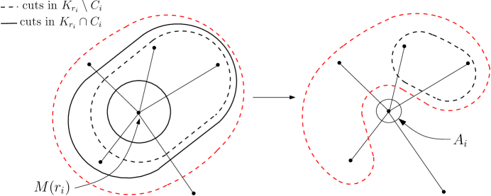
Figure 2: An iteration of algorithm Round-2 (Steps 3b & 3d)

For a terminal $i$ and edge $e$, if at the time that $i$ is picked in Step 3a of the algorithm $e$ is in $\delta(M(r_{i}))$, we say that $i$ accesses $e$. If $e\in E_{i}$, we say that $i$ defaults on $e$, and if $e$ is in $\delta(A_{i})$ after this iteration, then we say that $i$ loads $e$.

During the course of the algorithm integral loads on edges increase, but fractional loads may increase or decrease. To study how these edge loads change during the course of the algorithm, we divide edges into five sets. Let $X_{-1}$ denote the set of edges with ${{\ell_{e}^{{\mathcal{A}}}}}\leq c_{e}-1$ and ${{\ell_{e}^{{\mathcal{C}}}}}>0$. For $a\in\{0,1\}$, let $X_{a}$ denote the set of edges with ${{\ell_{e}^{{\mathcal{A}}}}}=c_{e}+a$ and ${{\ell_{e}^{{\mathcal{C}}}}}>0$. $Y$ denotes the set of edges with ${{\ell_{e}^{{\mathcal{A}}}}}\geq c_{e}+2$ and ${{\ell_{e}^{{\mathcal{C}}}}}>0$, and $Z$ denotes the set of edges with ${{\ell_{e}^{{\mathcal{C}}}}}=0$. Every edge starts out with a zero integral load. As the algorithm proceeds, the edge goes through one or more of the $X_{a}$s, may enter the set $Y$, and eventually ends up in the set $Z$. As for the CSCP, when an edge enters $Z$, we merge the end-points of the edge into a single meta-node. However, unlike for the CSCP, edges may get loaded even after entering $Z$. When an edge enters $Y$, we avoid loading it further (Step 3c), and instead load some edges in $Z$. Nevertheless, we ensure that edges in $Z$ are loaded no more than once.

As before our analysis has two components. First we show (Lemma 8) that the cuts produced by the algorithm are feasible. The following lemmas give the desired guarantees on the edges’ final loads: Lemmas 9 and 10 analyze the loads of edges in $X_{a}$ for $a\in\{-1,0,1\}$; Lemma 11 analyzes edges in $Y$ and Lemmas 12 and 13 analyze edges in $Z$. We put everything together in the proof of Lemma 4 at the end of this section.

  Input: Graph $G=(V,E)$ with capacities $c_{e}$ on edges, a set of terminals $T$ with a fractional laminar cut family ${\mathcal{C}}$.
Output: A collection of cuts ${\mathcal{A}}$, one for each terminal in $T$.
 

1. Preprocess the family ${\mathcal{C}}$ so that it satisfies the inclusion invariant.

2. Initialize $T^{\prime}=T$, ${\mathcal{A}}=\emptyset$, $Y,Z=\emptyset$, and $M(v)=\{v\}$ for all $v\in V$.

3. While there are terminals in $T^{\prime}$ do:

   1. Consider the set of unassigned terminals with the maximum depth, and of these let $i\in T^{\prime}$ be a terminal that is undominated in the cut inclusion ordering. Let $E_{i}=Y\cap\delta(M(r_{i}))$.

   2. If $E_{i}=\emptyset$, let $A_{i}=M(r_{i})$.

   3. If $E_{i}\neq\emptyset$ (we say that the terminal has “defaulted” on edges in $E_{i}$), let $U_{i}$ denote the set of end-points of edges in $E_{i}$ that lie in $M(r_{i})$. If $r_{i}\in U_{i}$, abort and return error. Otherwise, consider the vertex in $U_{i}$ that entered $M(r_{i})$ first during the algorithm’s execution, call this vertex $u_{i}$. Set $A_{i}$ to be the meta-node of $r_{i}$ just prior to the iteration where $M(u_{i})$ becomes equal to $M(r_{i})$.

   4. Add $A_{i}$ to ${\mathcal{A}}$. Remove ${\mathcal{C}}_{i}$ from ${\mathcal{C}}$ and $i$ from $T^{\prime}$. For every $j\in T^{\prime}$ and $C\in K_{r_{i}}^{1}\cap{\mathcal{C}}_{j}$, let $C=C\setminus\{M(r_{i})\}$.

   5. If for some edge $e$, ${{\ell_{e}^{{\mathcal{A}}}}}=c_{e}+2$ and ${{\ell_{e}^{{\mathcal{C}}}}}>0$, add $e$ to $Y$. If there exists an edge $e=(u,v)$ with ${{\ell_{e}^{{\mathcal{C}}}}}=0$, merge the meta-nodes $M(u)$ and $M(v)$ (we say that the edge $e$ has been “contracted”.) Add all edges $e$ with ${{\ell_{e}^{{\mathcal{C}}}}}=0$ to $Z$ and remove them from $Y$.

   6. Recompute the depths of vertices and terminals.

 

Figure 3: Algorithm Round-2—Rounding algorithm for multiway cut packing

Lemma 8

For all $i$, $r_{i}\in A_{i}\subseteq O_{i}$.

Proof.

Each cut $A_{i}$ is set equal to the meta-node of $r_{i}$ at some stage of the algorithm. Therefore, $r_{i}\in A_{i}$ for all $i$. Furthermore, at the time that $i$ is assigned an integral cut, $A_{i}\subseteq M(r_{i})\subseteq O_{i}$. ∎

Next we prove some facts about the fractional and integral loads as an edge goes through the sets $X_{a}$. The proofs of the following two lemmas are similar to that of Lemma 7.

Lemma 9

At any point of time, for every edge $e\in X_{-1}$, ${{\ell_{e}^{{\mathcal{A}}}}}+{{\ell_{e}^{{\mathcal{C}}}}}\leq c_{e}$.

Proof.

We prove the claim by induction over time. Note that in the beginning of the algorithm, we have for all edges ${{\ell_{e}^{{\mathcal{C}}}}}\leq c_{e}$ and ${{\ell_{e}^{{\mathcal{A}}}}}=0$, so the inequality ${{\ell_{e}^{{\mathcal{A}}}}}+{{\ell_{e}^{{\mathcal{C}}}}}\leq c_{e}$ holds.

Let us now consider a single iteration of the algorithm and suppose that the edge $e$ remains in the set $X_{-1}$ after this step. There are three events that influence the load of the edge $e=(u,v)$: (1) a terminal at some vertex in $M(u)$ accesses $e$; (2) a terminal at $M(v)$ accesses $e$; and, (3) a terminal at some other meta-node $M\neq M(u),M(v)$ is assigned an integral cut. Let us consider the third case first, and suppose that a terminal $i$ is assigned. Since $A_{i}\subseteq M$ and therefore $e\notin\delta(A_{i})$ its integral load does not increase. However, in the event that $S_{e}\cap{\mathcal{C}}_{i}$ is non-empty, the fractional load on $e$ may decrease (because cuts in ${\mathcal{C}}_{i}$ are removed from ${\mathcal{C}}$). Therefore, the inequality continues to hold.

Next we consider the case where a terminal, say $i$, with $r_{i}\in M(u)$ accesses $e$ (the second case is similar). Note that $M(r_{i})=M(u)$. In this case the integral load of the edge $e$ potentially increases by $1$ (if the terminal loads the edge). By the definition of $X_{-1}$, the new integral load on this edge is no more than $c_{e}-1$. The fractional load on $e$ changes in three ways:

• Cuts in ${\mathcal{C}}_{i}\cap S_{e}$ are removed from ${\mathcal{C}}$, decreasing ${{\ell_{e}^{{\mathcal{C}}}}}$.

• Some of the cuts in $(K_{r_{i}}^{1}\setminus{\mathcal{C}}_{i})\setminus S_{e}$ get “shifted” on to $e$ increasing ${{\ell_{e}^{{\mathcal{C}}}}}$ (we remove the meta-node $M(r_{i})$ from these cuts, and they may continue to contain $M(v)$).

• Cuts in $(K_{r_{i}}^{1}\setminus{\mathcal{C}}_{i})\cap S_{e}$ get shifted off from $e$ decreasing ${{\ell_{e}^{{\mathcal{C}}}}}$ (these cuts initially contain $M(r_{i})$ but not $M(v)$, and during this step we remove $M(r_{i})$ from these cuts).

So the decrease in ${{\ell_{e}^{{\mathcal{C}}}}}$ is at least the total weight of $K_{r_{i}}^{1}\cap S_{e}=K_{u}^{1}\cap S_{e}$, whereas the increase is at most the total weight of $K_{r_{i}}^{1}\setminus S_{e}=K_{u}^{1}\setminus S_{e}$.

In order to account for the two terms, let $\alpha$ denote the total weight of cuts in $K_{u}\cap S_{e}$, and $\beta$ denote the total weight of cuts in $K_{v}\cap S_{e}$. Then, $\alpha+\beta={{\ell_{e}^{{\mathcal{C}}}}}$. As in the proof of Lemma 7, we have $d_{v}=d_{u}-\alpha+\beta$, and therefore $d_{u}\geq d_{v}$ implies $\alpha\geq\beta$. Now, suppose that $\alpha\geq 1$. Then $K_{u}^{1}\subseteq S_{e}$. Therefore, the decrease in ${{\ell_{e}^{{\mathcal{C}}}}}$ due to the sets $K_{u}^{1}\cap S_{e}=K_{u}^{1}$ is at least $1$, and there is no corresponding increase, so the sum ${{\ell_{e}^{{\mathcal{A}}}}}+{{\ell_{e}^{{\mathcal{C}}}}}$ remains at most $c_{e}$.

Finally, suppose that $\alpha<1$. Then $K_{u}^{1}$ contains all the cuts in $K_{u}\cap S_{e}$, the weight of $K_{u}^{1}\cap S_{e}$ is exactly $\alpha$, and so the decrease in ${{\ell_{e}^{{\mathcal{C}}}}}$ is at least $\alpha$. Moreover, the total weight of $K_{u}^{1}\setminus S_{e}$ is $1-\alpha$, therefore, the increase in ${{\ell_{e}^{{\mathcal{C}}}}}$ due to the sets in $K_{u}^{1}\setminus S_{e}$ is at most $1-\alpha$. Since ${{\ell_{e}^{{\mathcal{C}}}}}$ starts out as being equal to $\alpha+\beta$, its final value after this step is $1-\alpha+\beta\leq 1$ as $\beta\leq\alpha$. Noting that ${{\ell_{e}^{{\mathcal{A}}}}}$ is at most $c_{e}-1$ after the step, we get the desired inequality. ∎

Lemma 10

For any edge $e=(u,v)$, from the time that $e$ enters $X_{0}$ to the time that it exits $X_{1}$, ${{\ell_{e}^{{\mathcal{C}}}}}\leq 1$. Furthermore suppose (without loss of generality) that during this time in some iteration $e$ is accessed by a terminal $i$ with $r_{i}\in M(u)$, then following this iteration until the next time that $e$ is accessed, we have $S_{e}\cap K_{u}=\emptyset$, and the next access to $e$ (if any) is from a terminal in $M(v)$.

Proof.

First we note that if the lemma holds the first time an edge $e=(u,v)$ enters a set $X_{a}$, $a\in\{0,1\}$, then it continues to hold while the edge remains in $X_{a}$. This is because during this time the integral load on the edge does not increase, and therefore throughout this time we assign integral cuts to terminals at meta-nodes different from $M(u)$ and $M(v)$ — this only reduces the fractional load on the edge $e$ and shrinks the set $S_{e}$.

Consider the first time that an edge $e=(u,v)$ moves from the set $X_{-1}$ to $X_{0}$. Suppose that at this step we assign an integral cut to a terminal $i$ residing at node $r_{i}\in M(u)$. Prior to this step, ${{\ell_{e}^{{\mathcal{A}}}}}=c_{e}-1$, and so by Lemma 9, ${{\ell_{e}^{{\mathcal{C}}}}}\leq 1$. As before define $\alpha$ to be the total weight of cuts $K_{u}\cap S_{e}$, and $\beta$ to be the total weight of cuts $K_{v}\cap S_{e}$. Then following the same argument as in the proof of Lemma 9, we conclude that the final fractional weight on $e$ is at most $\beta+1-\alpha\leq 1$. Furthermore, since $K_{u}\cap S_{e}\subseteq K_{u}^{1}$, we either remove all these cuts from ${\mathcal{C}}$ or shift them off of edge $e$. Moreover, any new cuts that we shift on to $e$ do not contain the meta-node $M(r_{i})=M(u)$, and in particular do not contain the vertex $u$. Therefore at the end of this step, $S_{e}\cap K_{u}=\emptyset$. This also implies that following this iteration terminals in $M(v)$ have depth larger than terminals in $M(u)$, and so the next access to $e$ must be from a terminal in $M(v)$.

The same argument works when an edge moves from $X_{0}$ to $X_{1}$. We again make use of the fact that prior to the step the fractional load on the edge is at most $1$. ∎

Lemma 11

During any iteration of the algorithm, for any edge $e\in Y$, the following are satisfied:

• ${{\ell_{e}^{{\mathcal{C}}}}}\leq 1$

• If the edge $e=(u,v)$ is accessed by a terminal $i$ with $r_{i}\in M(u)$, then following this iteration until the next time that $e$ is accessed, we have $S_{e}\cap K_{u}=\emptyset$, and the next access to $e$ (if any) is from a terminal in $M(v)$.

• If a terminal $i$ with $r_{i}\in M(u)$ accesses $e=(u,v)$, then $r_{i}\neq u$, $A_{i}\cap\{u,v\}=\emptyset$, and so $i$ does not load $e$. Also, consider any previous access to the edge by a terminal in $M(u)$; then prior to this access, $r_{i}\not\in M(u)$.

Proof.

The first two parts of this lemma extend Lemma 10 to the case of $e\in Y$, and are otherwise identical to that lemma. The proof for these claims is analogous to the proof of Lemma 10. The only difference is that terminals accessing an edge $e\in Y$ default on this edge. However, this does not affect the argument: when a terminal defaults on the edge, the edge’s fractional load changes in the same way as if the terminal did not default; the only change is in the way an integral cut is assigned to the terminal. Since these claims depend only on how the fractional load on the edge changes, they continue to hold while the edge is in $Y$.

For the third part of the lemma, since $A_{i}\subseteq M(r_{i})=M(u)$ and $v\not\in M(u)$, $v\not\in A_{i}$. Next we show that $u\not\in A_{i}$. Consider the iterations of the algorithm during which ${{\ell_{e}^{{\mathcal{C}}}}}\leq 1$. During this time the edge was accessed at least twice prior to being accessed by $i$ (once when $e$ moved from $X_{0}$ to $X_{1}$, once when $e$ moved from $X_{1}$ to $Y$, and possibly multiple times while $e\in Y$). Let the last two accesses be by the terminals $j_{1}$ and $j_{2}$, at iterations $t_{1}$ and $t_{2}$, $t_{1}\leq t_{2}$. For $a\in\{0,1\}$, let $M^{a}(u)$ and $M^{a}(v)$ denote the meta-nodes of $u$ and $v$ respectively just prior to iteration $t_{a}$, and $M(u)$ and $M(v)$ denote the respective meta-nodes just prior to the current iteration. Then by Lemma 10 and the second part of this lemma, we have $r_{j_{1}}\in M^{1}(u)$ and $r_{j_{2}}\in M^{2}(v)$. We claim that $i>_{CI}j_{2}>_{CI}j_{1}$. Given this claim, if $r_{i}\in M^{1}(u)=M^{1}(r_{j_{1}})$, then since $i$ and $j_{1}$ have the same depth at iteration $t_{1}$, we get a contradiction to the fact that the algorithm picks $j_{1}$ before $i$ in Step 3a. Therefore, $r_{i}\not\in M(u)$ at any iteration prior to $t_{1}$, and in particular, $r_{i}\neq u$. Finally, since $u\in U_{i}$ and $U_{i}\cap A_{i}=\emptyset$, this also implies that $u\not\in A_{i}$.

It remains to prove the claim. We will prove that $j_{2}>_{CI}j_{1}$. The proof for $i>_{CI}j_{2}$ is analogous. In fact we will prove a stronger statement: between iterations $t_{1}$ and $t_{2}$, all terminals with cuts in $S_{e}$ dominate $j_{1}$ in the cut-inclusion ordering. We prove this by induction. By Lemma 10, prior to iteration $t_{1}$, $S_{e}$ does not contain any cuts belonging to terminals at $M(v)$. Following the iteration, $S_{e}$ only contains fractional cuts in $K_{u}^{1}$ that got shifted on to the edge $e$. Prior to shifting, these cuts contain $M^{1}(u)$, and therefore $r_{j_{1}}$, but do not belong to $j_{1}$. Then, these cuts are subsets of $O_{j_{1}}$, and so by the inclusion invariant, they belong to terminals dominating $j_{1}$ in the cut-inclusion ordering. Therefore, the claim holds right after the iteration $t_{1}$. Finally, following the iteration until the next time that $e$ is accessed (by $j_{2}$), the set $S_{e}$ only shrinks, and so the claim continues to hold. ∎

In order to analyze the loading of edges in $Z$, we need some more notation. Let ${\mathcal{M}}$ denote the collection of sets of vertices that were meta-nodes at some point during the algorithm. For any edge $e\in Z$, let $M_{e}$ denote the meta-node formed when $e$ enters $Z$; then $M_{e}$ is the smallest set in ${\mathcal{M}}$ containing both the end points of $e$. Note that the collection ${\mathcal{A}}\cup{\mathcal{M}}$ is laminar.

Lemma 12

An edge $e\in Z$ is loaded only if after the formation of $M_{e}$ a terminal residing at a vertex in $M_{e}$ defaults on an edge in $\delta(M_{e})$. (Note that this may happen after $M_{e}$ has merged with some other meta-nodes.)

Proof.

Let $i$ be a defaulting terminal that loads the edge $e\in Z$. Then $e\in\delta(A_{i})$, and therefore, $A_{i}\subsetneq M_{e}$ and $r_{i}\in M_{e}$. Furthermore, since $A_{i}$ is a strict subset of $M_{e}$, $U_{i}\cap M_{e}\neq\emptyset$, and therefore, $i$ defaults on an edge $e^{\prime}\in Y$ with at least one end-point in $M_{e}$. But if both the end-points of $e^{\prime}$ are in $M_{e}$, then we must have $\ell_{e^{\prime}}^{{\mathcal{C}}}=0$ contradicting the fact that $e^{\prime}$ is in $Y$. Therefore, $e^{\prime}\in\delta(M_{e})$. ∎

Lemma 13

For any meta-node $M\in{\mathcal{M}}$, after its formation, at most one terminal residing at a vertex in $M$ can default on edges in $\delta(M)$ (even after $M$ has merged with other meta-nodes).

Proof.

For the sake of contradiction, suppose that two terminals $i$ and $j$, both residing at vertices in $M$ default on edges in $\delta(M)$ after the formation of $M$, with $i$ defaulting before $j$. Let $M_{1}$ ($M_{2}$) denote the meta-node containing $M$ just before $i$ ($j$) defaulted. Note that $M\subseteq M_{1}\subseteq M_{2}$. Consider an edge $e\in E_{j}\cap\delta(M)$ (recall that $E_{j}$ is the set of edges that $j$ defaults on, so this set is non-empty by our assumption). Then $e\in\delta(M)\cap\delta(M_{2})\subseteq\delta(M_{1})$. Therefore, at the time that $i$ defaulted, $e$ was accessed by $i$, and by the third claim in Lemma 11, $r_{j}\not\in M_{1}$. This contradicts the fact that $r_{j}\in M$. ∎

Finally we can put all these lemmas together to prove our main result on algorithm Round-2.

Lemma 4

Given a fractional laminar cut family ${\mathcal{C}}$ feasible for the MCP on a graph $G$ with integral edge capacities $c_{e}$, the algorithm Round-2 produces an integral family of cuts ${\mathcal{A}}$ that is feasible for the MCP on $G$ with edge capacities $c_{e}+3$.

Proof.

We first note that the third part of Lemma 11 implies that for all $i$, $r_{i}\not\in U_{i}$, and therefore the algorithm never aborts. Then Lemma 8 implies that we get a feasible cut packing. Finally, note that every edge starts out in the set $X_{-1}$, goes through one or more of the $X_{a}$’s, $a\in\{0,1\}$, potentially goes through $Y$, and ends up in $Z$. An edge $e$ enters $Y$ when its integral load becomes $c_{e}+2$. Lemma 11 implies that edges in $Y$ never get loaded, and so at the time that an edge $e$ enters $Z$, ${{\ell_{e}^{{\mathcal{A}}}}}\leq c_{e}+2$. After this point the edge stays in $Z$, and Lemmas 12 and 13 imply that it gets loaded at most once. Therefore, the final load on the edge is at most $c_{e}+3$. ∎

4 Constructing fractional laminar cut packings

We now show that fractional solutions to the program MCP-LP can be converted in polynomial time into fractional laminar cut families while losing only a small factor in edge load. We begin with the common sink case.

  Input: Graph $G=(V,E)$ with edge capacities $c_{e}$, commodities $S_{1},\cdots,S_{k}$, common sink $t$, a feasible solution $d$ to the program MCP-LP.
Output: A fractional laminar family of cuts ${\mathcal{C}}$ that is feasible for $G$ with edge capacities $c_{e}+o(1)$.
 

1. For every $a\in[k]$ and terminal $i\in S_{a}$ do the following: Order the vertices in $G$ in increasing order of their distance under $d_{a}$ from $r_{i}$. Let this ordering be $v_{0}=r_{i},v_{1},\cdots,v_{n}$. Let ${\mathcal{C}}_{i}$ be the collection of cuts $\{v_{0},v_{1},\cdots,v_{b}\}$, one for each $b\in[n]$, $d_{a}(r_{i},v_{b})<1$, with weights $w(\{v_{0},\cdots,v_{b}\})=d_{a}(r_{i},v_{b+1})-d_{a}(r_{i},v_{b})$. Let ${\mathcal{C}}$ denote the collection $\{{\mathcal{C}}_{i}\}_{i\in\cup_{a}S_{a}}$.

2. Let $N=nk$. Round up the weights of all the cuts in ${\mathcal{C}}$ to multiples of $1/N^{2}$, and truncate the collection so that the total weight of every sub-collection ${\mathcal{C}}_{i}$ is exactly $1$. Also split every cut with weight more than $1/N^{2}$ into multiple cuts of weight exactly $1/N^{2}$ each, assigned to the same commodity.

3. While there are pairs of cuts in ${\mathcal{C}}$ that cross, consider any pair of cuts $C_{i},C_{j}\in{\mathcal{C}}$ belonging to terminals $i\neq j$ that cross each other. Transform these cuts into new cuts for $i$ and $j$ according to Figure 5.

 

Figure 4: Algorithm Lam-1—Algorithm to convert an LP solution for the CSCP into a feasible fractional laminar family

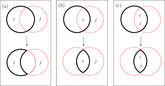
Figure 5: Rules for transforming an arbitrary cut family into a laminar one for the CSCP. The dark cuts in this figure correspond to the terminal $i$, and the light cuts to terminal $j$; $t$ lies outside all the cuts.

4.1 Obtaining laminarity in the common sink case

We prove Lemma 1 in this section. Our algorithm involves starting with a solution to MCP-LP, converting it into a feasible fractional non-laminar family of cuts, and then resolving pairs of crossing cuts one at a time by applying the rules in Figure 5. The algorithm is given in Figure 4.

Lemma 1

Consider an instance of the CSCP with graph $G=(V,E)$, common sink $t$, edge capacities $c_{e}$, and commodities $S_{1},\cdots,S_{k}$. Given a feasible solution $d$ to MCP-LP, algorithm Lam-1 produces in polynomial time a fractional laminar cut family ${\mathcal{C}}$ that is feasible for the CSCP on $G$ with edge capacities $c_{e}+o(1)$.

Proof.

We first note that the family ${\mathcal{C}}$ is feasible for the given instance of CSCP at the end of Step 2, but is not necessarily laminar. Since the number of distinct cuts in ${\mathcal{C}}$ after Step 1 is at most $nk=N$, at the end of Step 2, edge loads are at most $c_{e}+1/N$. As we tranform the cuts in Step 3, we maintain the property that no cut $C\in{\mathcal{C}}$ contains the sink $t$, but every cut $C\in{\mathcal{C}}_{i}$ contains the node $r_{i}$ for terminal $i$. It is also easy to see from Figure 5 that the load on every edge stays the same. Finally, in every iteration of this step, the number of pairs of crossing cuts strictly decreases. Therefore, the algorithm ends after a polynomial number of iterations. ∎

4.2 Obtaining laminarity in the general case

Obtaining laminarity in the general case involves a more careful selection and ordering of rules of the form given in Figure 5. The key complication in this case is that we must maintain separation of every terminal from every other terminal in its commodity set. We first show how to convert an integral collection of cuts feasible for the MCP into a feasible integral laminar collection of cuts. We lose a factor of $2$ in edge loads in this process (see Lemma 14 below). Obtaining laminarity for an arbitrary fractional solution requires converting it first into an integral solution for a related cut-packing problem and then applying Lemma 14 (see algorithm Lam-2 in Figure 8 and the proof of Lemma 2 following it).

Lemma 14

Consider an instance of the MCP with graph $G=(V,E)$and commodities $S_{1},\cdots,S_{k}$, and let ${\mathcal{C}}^{1}=\{C^{1}_{i}\}_{i\in S_{a},a\in[k]}$ be a family of cuts such that for each $a\in[k]$ and $i\in S_{a}$, $C^{1}_{i}$ contains $i$ but no other $j\in S_{a}$. Then algorithm Integer-Lam-2 produces a laminar cut collection ${\mathcal{C}}^{2}=\{C^{2}_{i}\}_{i\in S_{a},a\in[k]}$ such that for each $a\in[k]$ and $i\neq j\in S_{a}$, either $C^{2}_{i}$ or $C^{2}_{j}$ separates $i$ from $j$, and ${\ell_{e}^{{\mathcal{C}}^{1}}}\leq 2{\ell_{e}^{{\mathcal{C}}^{2}}}$ for every edge $e\in E$.

In the remainder of this section we interpret cuts as sets of vertices as well as sets of terminals residing at those vertices. The algorithm for laminarity in the integral case is given in Figure 6.

  Input: Graph $G=(V,E)$ with edge capacities $c_{e}$, commodities $S_{1},\cdots,S_{k}$, a family of cuts ${\mathcal{C}}$ with one cut for every terminal in $\cup_{a}S_{a}$, such that the cut for terminal $i\in S_{a}$ does not contain any terminal $j\neq i$ in $S_{a}$.
Output: A laminar collection of cuts, one for each terminal in $\cup_{a}S_{a}$, such that for all $a$ and for all $i,j\in S_{a}$, $i\neq j$, either the cut for $i$ or the cut for $j$ separates $i$ from $j$.
 

1. While there are pairs of cuts in ${\mathcal{C}}$ that cross, do (see Figure 7):

   1. Consider any pair of cuts $C_{i},C_{j}\in{\mathcal{C}}$ belonging to terminals $i\neq j$ that cross each other, such that $r_{i}\in C_{i}\setminus C_{j}$ and $r_{j}\in C_{j}\setminus C_{i}$. Reassign $C_{i}=C_{i}\setminus C_{j}$ and $C_{j}=C_{j}\setminus C_{i}$. Return to Step 1.

   2. Consider any three terminals $i_{1},i_{2},i_{3}$ with cuts $C_{1},C_{2}$ and $C_{3}$ such that $r_{i_{1}}\in C_{1}\cap C_{2}\setminus C_{3}$, $r_{i_{2}}\in C_{2}\cap C_{3}\setminus C_{1}$, and $r_{i_{3}}\in C_{3}\cap C_{1}\setminus C_{2}$. Then, reassign these respective intersections to the three terminals. Return to Step 1.

   3. Consider any pair of cuts $C_{i},C_{j}\in{\mathcal{C}}$ belonging to terminals $i,j\in S_{a}$ for some $a$ that cross each other, such that $r_{i}\in C_{i}\cap C_{j}$ and $r_{j}\in C_{j}\setminus C_{i}$. Reassign $C_{i}=C_{i}\cap C_{j}$ and $C_{j}=C_{i}\cup C_{j}$. Return to Step 1.

   4. Consider any pair of cuts $C_{i},C_{j}\in{\mathcal{C}}$ belonging to terminals $i\neq j$ that cross each other, such that $r_{i},r_{j}\in C_{i}\cap C_{j}$, $i\in S_{a}$ and $j\in S_{b}$ with $a\neq b$.

      • Suppose that there is no $i^{\prime}\in S_{a}\cap C_{j}$ with $C_{i}\subset C_{i^{\prime}}$. Then, reassign $C_{i}=C_{i}\cup C_{j}$ and $C_{j}=C_{i}\cap C_{j}$; return to Step 1. Conversely, if there is no $j^{\prime}\in S_{b}\cap C_{i}$ with $C_{j}\subset C_{j^{\prime}}$. Then, reassign $C_{j}=C_{i}\cup C_{j}$ and $C_{i}=C_{i}\cap C_{j}$; return to Step 1. (This transformation is similar to Step 1c.)

      • If neither of those cases hold, let $i_{0}=i$, and let $i_{1},\cdots,i_{x}$ denote the terminals in $S_{a}\cap C_{j}$ with $C_{i}\subset C_{i_{1}}\subset C_{i_{2}}\subset\cdots\subset C_{i_{x}}$. For $x^{\prime}\leq x-2$, reassign $C_{i_{x^{\prime}}}=(C_{i_{x^{\prime}+1}}\setminus C_{j})\cup C_{i_{x^{\prime}}}$, $C_{i_{x-1}}=C_{i_{x}}\cup C_{j}$, and $C_{i_{x}}=C_{i_{x}}\cap C_{j}\setminus C_{i_{x-1}}$. Reassign cuts to $j$ and terminals in $S_{b}\cap C_{i}$ likewise. Return to Step 1.

   5. If none of the above rules match, then go to Step 2.

2. Let ${\mathcal{G}}$ be a directed graph on the vertex set $\cup_{a}S_{a}$, with edges colored red or blue, defined as follows: for terminals $i\neq j$, ${\mathcal{G}}$ contains a red edge from $i$ to $j$ if and only if $C_{j}\subset C_{i}$, and contains a blue edge from $i$ to $j$ if and only if $r_{j}\in C_{i}$, $r_{i}\not\in C_{j}$, and $C_{j}\setminus C_{i}\neq\emptyset$. We note that since no pair of terminals $i$ and $j$ matches the rules in Step 1, whenever $C_{i}$ and $C_{j}$ intersect ${\mathcal{G}}$ contains an edge between $i$ and $j$.

   While there is a directed blue cycle in ${\mathcal{G}}$, consider the shortest such cycle $i_{1}\rightarrow i_{2}\rightarrow\cdots\rightarrow i_{x}\rightarrow i_{1}$. For $x^{\prime}\leq x$, $x^{\prime}\neq 1$, assign to $i_{x^{\prime}}$ the cut $C_{i_{x^{\prime}}}\cap C_{i_{x^{\prime}-1}}$, and assign to $i_{1}$ the cut $C_{i_{1}}\cap C_{i_{x}}$.

3. We show in Lemma 15 that at this step ${\mathcal{G}}$ is acyclic. For every connected component in ${\mathcal{G}}$ do:

   1. Let $T$ be the set of terminals in the component and $A$ be the set of corresponding cuts. Assign capacities $p_{e}=2{\ell_{e}^{A}}$ to edges in $G$. Let $G_{p}$ be the graph obtained by merging all pairs of vertices that have an edge $e$ with $p_{e}=0$ between them. We call the vertices of $G_{p}$ “meta-nodes” (note that these are sets of vertices in the original graph). At any point of time, let $R_{i}$ denote the meta-node at which a terminal $i$ resides.

   2. While there are terminals in $T$, pick any “leaf” terminal $i$ (that is, a terminal with no outgoing red or blue edges in ${\mathcal{G}}$). Reassign to $i$ the cut $R_{i}$. Reduce the capacity of every edge $e\in\delta(R_{i})$ by $1$. Remove $i$ from $T$; remove $i$ and all edges incident on it from ${\mathcal{G}}$. Recompute the graph $G_{p}$ based on the new capacities.

 

Figure 6: Algorithm Integer-Lam-2—Algorithm to convert an integral family of multiway cuts into a laminar one

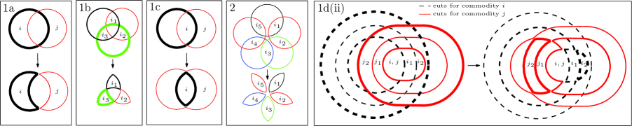
Figure 7: Some simple rules for resolving crossing cuts. See algorithm Integer-Lam-2 in Figure 6 for formal descriptions.

As in the common sink case, the algorithm starts by applying a series of simple rules to pairs of crossing cuts while maintaining the invariant that pairs of terminals belonging to the same commodity are always separated by at least one of the two cuts assigned to them. Certain kinds of crossings of cuts are easy to resolve while maintaining this invariant (Step 1 of the algorithm resolves these crossings; see also Figure 7). In Steps 2 and 3, we ignore the commodities that each terminal belongs to, and assign new laminar cuts to terminals while ensuring that the new cut of each terminal lies within its previous cut (and therefore, separation continues to be maintained). These steps incur a penalty of $2$ in edge loads.

The rough idea behind Steps 2 and 3 is to consider the set of all “conflicting” terminals, call it $F$. Then we can assign to each terminal $i\in F$ the cut $\cap_{j\in F}\hat{C}_{j}$ where $\hat{C}_{j}$ is either the cut of terminal $j$ or its complement depending on which of the two contains $r_{i}$. These intersections are clearly laminar, and are subsets of the original cuts assigned to terminals. Furthermore, if each terminal gets a unique intersection, then edge loads increase by a factor of at most $2$. Unfortunately, some groups of terminals may share the same intersections. In order to get around this, we assign cuts to terminals in a particular order suggested by the structure of the conflict graph on terminals (graph ${\mathcal{G}}$ in the algorithm) and assign appropriate intersections to them while explicitly ensuring that edge loads increase by a factor of no more than $2$.

Throughout the algorithm, every terminal in $\cup_{a}S_{a}$ has an integral cut assigned to it. The proof of Lemma 14 is established in three parts: Lemma 15 establishes the laminarity of the output cut family, Lemma 17 argues separation, and Lemma 18 analyzes edge loads.

Lemma 15

Algorithm Integer-Lam-2 runs in polynomial time and produces a laminar cut collection.

Proof.

As in the previous section define the crossing number of a family of cuts to be the number of pairs of cuts that cross each other. We first note that in every iteration of Steps 1 and 2 of the algorithm, the crossing number of the cut family ${\mathcal{C}}$ strictly decreases: no new crossings are created in these steps, while the crossings of the two or more cuts involved in each transformation are resolved (see Figure 7). Therefore, after a polynomial number of steps, we exit Steps 1 and 2 and go to Step 3.

Next, we claim that during Step 3 of the algorithm the graph ${\mathcal{G}}$ is acyclic. This implies that while ${\mathcal{G}}$ is non-empty, we can always find a leaf terminal in Step 3; therefore every terminal in ${\mathcal{G}}$ gets assigned a new cut. It is immediate that the graph does not contain any directed blue cycles or any directed red cycles (the latter follows because red edges define a partial order over terminals). Suppose the graph contains three terminals $i_{1}$, $i_{2}$ and $i_{3}$ with a red edge from $i_{1}$ to $i_{2}$, and a red or blue edge from $i_{2}$ to $i_{3}$, then it is easy to see that there must be a red or blue edge from $i_{1}$ to $i_{3}$. Therefore, any multi-colored directed cycle must reduce to either a smaller blue cycle or a cycle of length $2$. Neither of these cases is possible (the latter is ruled out by definition), and therefore the graph cannot contain any multi-colored cycles.

Now consider cuts assigned during Step 3. Let $T$ be the set of terminals corresponding to some component in ${\mathcal{G}}$ and $j\not\in T$. Then before $T$ is processed, $j$’s cut is laminar with respect to all the cuts in $A_{T}$, and is therefore a subset of some meta-node in $G_{p^{T}}$. So the new cuts assigned to terminals in $T$ are also laminar with respect to $j$’s cut.

Finally, consider any two cuts assigned during Step 3 of the algorithm and belonging to two terminals in the same component of ${\mathcal{G}}$. Consider the set of all meta-nodes created during this iteration of Step 3. This set is laminar, and the cuts assigned during this iteration are a subset of this laminar family. Therefore, they are laminar. ∎

Lemma 16

For a commodity $i$ assigned a cut in Step 3 of algorithm Integer-Lam-2, let $C^{1}_{i}$ be its cut before this step, and $C^{2}_{i}$ be the new cut assigned to it. Then $C^{2}_{i}\subseteq C^{1}_{i}$.

Proof.

We assume without loss of generality that prior to Step 3 each edge load is at most one; this can be achieved by splitting a multiply-loaded edge into many edges. We focus on the behavior of the algorithm for a single component $T$ of ${\mathcal{G}}$ and prove the lemma by induction over time.

Consider an iteration of Step 3b during which some terminal $i\in T$ is assigned and let $C_{i}$ be its original cut. Consider any vertex $v\not\in C_{i}$ and let $P$ be a shortest simple path from $r_{i}$ to $v$ in $G_{p^{T}}$ (where the length of an edge $e$ is given by $p^{T}_{e}$ just prior to when $i$ is assigned a new cut). It is easy to see that there is one such shortest path that crosses each new cut assigned prior to this iteration in Step 3b at most twice – suppose there are multiple entries and exits for some cut, we can “short-cut” the path by connecting the first point on the path inside the cut to the last point on the path inside the cut via a simple path of length $0$ lying entirely inside the cut. We pick $P$ to be such a path. We will prove that $P$’s length is at least $2$. So the meta-node containing $i$ must lie inside the cut $C_{i}$, and the lemma holds.

Let $T_{1}$ (resp. $T_{2}$) be the set of terminals in $T\setminus C_{i}$ (resp. $T\cap C_{i}$) that are assigned new cuts before $i$ in this iteration. We first note that for any $j$ in $T_{1}$, prior to this step, there is no edge from $j$ to $i$ (as $j$ is assigned before $i$), so $r_{i}\not\in C_{j}$, and this along with $r_{j}\not\in C_{i}$ implies that $C_{i}$ and $C_{j}$ are disjoint. This implies that the new cut of $j$ (which is a subset of $C_{j}$ by induction) is also disjoint from $C_{i}$, and therefore cannot load any edge with an end-point in $C_{i}$. So the only new cuts assigned this far in Step 3b that load edges in $P$ belong to terminals in $T_{2}$.

Now we will analyze $P$’s length by accounting for all the newly assigned cuts that load its edges. Let $S_{P}$ be the set of terminals in $T_{2}$ that load an edge in $P$, and $j\in S_{P}$. Since the new cut of $j$ intersects $P$, by the induction hypothesis, $C_{j}$ should either intersect $P$ or contain the entire path inside it. If $C_{j}$ contains $P$ entirely, then $C_{j}\setminus C_{i}\neq\emptyset$, and furthermore $r_{i},r_{j}\in C_{i}\cap C_{j}$. This implies that either $C_{i}\subset C_{j}$ and there is a directed red edge from $j$ to $i$, or $C_{i}\setminus C_{j}\neq\emptyset$, that is, $C_{i}$ and $C_{j}$ cross and should have matched the rule in Step 1d of the algorithm. Both possibilities lead to a contradiction. Therefore, $C_{j}$ must intersect $P$.

Finally, the original total length of the path is at least $2|S_{P}|+2$, because each terminal in $S_{P}$ contributes two units towards its length, and another two units is contributed by $C_{i}$. Out of these up to $2|S_{P}|$ units of length is consumed by terminals in $S_{P}$. Therefore, at the time that $i$ is assigned a cut, at least $2$ units remain. ∎

Lemma 17

When algorithm Integer-Lam-2 terminates, for every $a\in[k]$ and $i\neq j\in S_{a}$, either $C_{i}$ or $C_{j}$ separates $i$ from $j$.

Proof.

We claim that for every $a\in[k]$ and $i\neq j\in S_{a}$, at every time step during the execution of the algorithm, $|C_{i}\cap C_{j}\cap\{r_{i},r_{j}\}|\leq 1$. Then since by Lemma 15 the final solution is laminar, the lemma follows. We prove this claim by induction over time. First, if during any iteration of the algorithm, we “shrink” the cut of any terminal (that is, reassign to the terminal a cut that is a strict subset of its original cut), then the claim continues to hold for that terminal, because intersections of the terminal’s cut only shrink in that step. Note that cuts of terminals expand only in Steps 1c and 1d of the algorithm (by construction and by Lemma 16).

Suppose that during some iteration we apply the transformation in Step 1c to terminals $i$ and $j$, reassigning $C_{j}=C_{i}\cup C_{j}$, and the claim fails to hold for terminal $j$. Specifically, suppose that for some $j^{\prime}\in S_{a}$, after the iteration we have $r_{j},r_{j^{\prime}}\in C_{j}\cap C_{j^{\prime}}$. Then, $r_{j}\in C_{j^{\prime}}$, and therefore $C_{j^{\prime}}$ intersected $C_{j}$ prior to the iteration, and by the induction hypothesis $r_{j^{\prime}}\in C_{i}\setminus C_{j}$ prior to the iteration. If $r_{i}\in C_{j^{\prime}}$, then prior to the iteration, $i$ and $j^{\prime}$ contradicted the induction hypothesis. Otherwise, $i$, $j$ and $j^{\prime}$ satisfy the conditions in Step 1b of the algorithm, and this contradicts the fact that we apply the transformation in Step 1c at this iteration.

Next suppose that during some iteration we apply the transformation in the first part of Step 1d to terminals $i$ and $j$, reassigning $C_{j}=C_{i}\cup C_{j}$, and the claim fails to hold for terminal $j$; in particular, for some $j^{\prime}\in S_{a}$, after the iteration we have $r_{j},r_{j^{\prime}}\in C_{j}\cap C_{j^{\prime}}$. Then, since $r_{j}\in C_{j^{\prime}}$ and the pair of terminals did not match the criteria in Step 1c, it must be the case that $C_{j}\subset C_{j^{\prime}}$ prior to the iteration. Furthermore, $r_{j^{\prime}}\in C_{i}$ prior to the iteration and this contradicts the fact that we applied the transformation in the first part of Step 1d.

Finally, suppose that during some iteration we apply the transformation in the second part of Step 1d. Then the cut assigned to every $i_{x^{\prime}}$ for $x^{\prime}\leq x-2$ is a subset of the previous cut of $i_{x^{\prime}+1}$, but does not contain the latter terminal, and so by the arguments presented for the previous cases, once again the induction hypothesis continues to hold for those terminals. Furthermore, the cut assigned to $i_{x}$ is a subset of its original cut and $i_{x-1}$ does not belong to any of the new cuts except its own. The same argument holds for the $j_{y^{\prime}}$ terminals. ∎

Lemma 18

For the cut collection produced by algorithm Integer-Lam-2 the load on every edge is no more than twice the load of the integral family of cuts input to the algorithm.

Proof.

We first claim that edge loads are preserved throughout Steps 1 and 2 of the algorithm. This can be established via a case-by-case analysis by noting that in every transformation of these steps, the number of new cuts that an edge crosses is no more than the number of old cuts that the edge crosses prior to the transformation. It remains to analyze Step 3 of the algorithm. We claim that we only lose a factor of $2$ in edge loads during this step of the algorithm. This is easy to see. Note that for every edge $e$, $\sum_{T}p^{T}_{e}\leq 2{\ell_{e}^{{\mathcal{C}}_{\cup T}}}$, where ${\mathcal{C}}_{\cup T}$ is the family of cuts belonging to terminals in any non-singleton component of ${\mathcal{G}}$ prior to Step 3. Moreover, in each iteration of the step, we only load an edge $e$ to the extent of $p^{T}_{e}$. Therefore the lemma follows. ∎

Proof of Lemma 14: The proof follows immediately from Lemmas 15, 17 and 18. ∎

Given this lemma, algorithm Lam-2 in Figure 8 converts an arbitrary feasible solution for MCP-LP into a feasible fractional laminar family.

  Input: Graph $G=(V,E)$ with edge capacities $c_{e}$, commodities $S_{1},\cdots,S_{k}$, a feasible solution $d$ to the program MCP-LP.
Output: A fractional laminar family of cuts ${\mathcal{C}}$ that is feasible for $G$ with edge capacities $8c_{e}+o(1)$.
 

1. For every $a\in[k]$ and every terminal $i\in S_{a}$ do the following: Order the vertices in $G$ in increasing order of their distance under $d_{a}$ from $r_{i}$. Let this ordering be $v_{0}=r_{i},v_{1},\cdots,v_{n}$. Let ${\mathcal{C}}^{1}_{i}$ be the collection of cuts $\{v_{0},v_{1},\cdots,v_{b}\}$, one for each $b\in[n]$ with $d_{a}(r_{i},v_{b})<0.5$, with weights $w^{1}(\{v_{0},\cdots,v_{b}\})=2(\min\{d_{a}(r_{i},v_{b+1}),0.5\}-d_{a}(r_{i},v_{b}))$. Let ${\mathcal{C}}^{1}$ denote the collection $\{{\mathcal{C}}^{1}_{i}\}_{i\in\cup_{a}S_{a}}$.

2. Let $N=n\sum_{a}|S_{a}|$. Round up the weights of all the cuts in ${\mathcal{C}}^{1}$ to multiples of $1/N^{2}$, and truncate the collection so that the total weight of every sub-collection ${\mathcal{C}}^{1}_{i}$ is exactly $1$. Furthermore, split every cut with weight more than $1/N^{2}$ into multiple cuts of weight exactly $1/N^{2}$ each, assigned to the same commodity. Call this new collection ${\mathcal{C}}^{2}$ with weight function $w^{2}$. Note that every cut in this collection has weight exactly $1/N^{2}$.

3. Construct a new instance of MCP in the same graph $G$ as follows. For each $a\in[k]$, construct $N^{2}$ new commodities with terminal sets identical to that of $S_{a}$ (that is the terminals reside at the same nodes). For every new terminal corresponding to an older terminal $i$, assign to the new terminal a unique cut from ${\mathcal{C}}^{2}_{i}$ with weight $1$. Call this new collection ${\mathcal{C}}^{3}$, and the new instance $I$.

4. Apply algorithm Integer-Lam-2 from Figure 6 to the family ${\mathcal{C}}^{3}$ to obtain family ${\mathcal{C}}^{4}$.

5. For every $a\in[k]$ and every $i\in S_{a}$, let ${\mathcal{C}}^{5}_{i}$ be the set of $N^{2}/2$ innermost cuts in ${\mathcal{C}}^{4}$ assigned to terminals in the new instance $I$ that correspond to terminal $i$. (Note that these cuts are concentric as they belong to a laminar family and all contain $r_{i}$. Therefore “innermost” cuts are well defined.) Assign a weight of $2/N^{2}$ to every cut in this set. Output the collection ${\mathcal{C}}^{5}$.

 

Figure 8: Algorithm Lam-2—Algorithm to convert an LP solution into a feasible fractional laminar family

Lemma 2

Consider an instance of the MCP with graph $G=(V,E)$, edge capacities $c_{e}$, and commodities $S_{1},\cdots,S_{k}$. Given a feasible solution $d$ to MCP-LP, algorithm Lam-2 produces a fractional laminar cut family ${\mathcal{C}}$ that is feasible for the MCP on $G$ with edge capacities $8c_{e}+o(1)$.

Proof.

Note first that the cut collection ${\mathcal{C}}^{1}$ satisfies the following properties: (1) For every $a\in[k]$ and $i\in S_{a}$, every cut in ${\mathcal{C}}^{1}_{i}$ contains $r_{i}$, but not $r_{j}$ for $j\in S_{a}$, $j\neq i$; (2) The total weight of cuts in $C^{1}_{i}$ is $1$; (3) For every edge $e$, ${\ell_{e}^{{\mathcal{C}}^{1}}}\leq 2\sum_{a}d_{a}(e)\leq 2c_{e}$. The family ${\mathcal{C}}^{2}$ also satisfies the first two properties, however loads the edges slightly more than ${\mathcal{C}}^{1}$. Any edge belongs to at most $N$ cuts, and therefore the load on the edge goes up by an additive amount of at most $1/N$. Therefore, for every $e$, ${\ell_{e}^{{\mathcal{C}}^{2}}}\leq 2c_{e}+1/N$. Next, the collection ${\mathcal{C}}^{3}$ is a feasible integral family of cuts for the new instance $I$ with ${\ell_{e}^{{\mathcal{C}}^{3}}}=N^{2}{\ell_{e}^{{\mathcal{C}}^{2}}}$. Therefore, applying Lemma 14, we get that ${\mathcal{C}}^{4}$ is a feasible laminar integral family of cuts for $I$ with ${\ell_{e}^{{\mathcal{C}}^{4}}}\leq 2N^{2}(2c_{e}+1/N)$. Finally, in family ${\mathcal{C}}^{5}$, every terminal $i\in S_{a}$ gets assigned $N^{2}/2$ fractional cuts, each with weight $2/N^{2}$. Therefore, the total weight of cuts in ${\mathcal{C}}^{5}_{i}$ is $1$. Now consider any two terminals $i,j\in S_{a}$ with $i\neq j$. Then, in all the $N^{2}$ commodities corresponding to $S_{a}$ in instance $I$, either the cut assigned to $i$’s counterpart, or that assigned to $j$’s counterpart separates $i$ from $j$. Say that among at least $N^{2}/2$ of the commodities in $I^{\prime}$, the cut assigned to $i$’s counterpart separates $i$ from $j$. Then, the innermost $N^{2}/2$ cuts assigned to $i$ in ${\mathcal{C}}^{5}$ separate $i$ from $j$. Therefore, the family ${\mathcal{C}}^{5}$ satisfies the first two conditions of feasibility as given in Definition 2. Finally, it is easy to see that on every edge $e$, ${\ell_{e}^{{\mathcal{C}}^{5}}}\leq 2/N^{2}{\ell_{e}^{{\mathcal{C}}^{4}}}\leq 4(2c_{e}+1/N)$. ∎

5 NP-Hardness

We will now prove that CSCP and MCP are NP-hard. Since edge loads for any feasible solution to these problems are integral, the result of Theorem 5 is optimal for the CSCP assuming P$\neq$NP. The reduction in this theorem also gives us an integrality gap instance for the CSCP.

Theorem 19

CSCP and MCP are NP-hard. Furthermore the integrality gap of MCP-LP is at least $2$ for both the problems.

Proof.

We reduce independent set to CSCP. In particular, given a graph $G$ and a target $k$, we produce an instance of CSCP such that the load on every edge is at most $1$ if and only if $G$ contains an independent set of size at least $k$. Let $n$ be the number of vertices in $G$. We construct $G^{\prime}$ by adding a chain of $n-k+1$ new vertices to $G$. Let the first vertex in this chain be $t$ (the common sink) and the last be $v$. We connect every vertex of $G$ to the new vertex $v$, and place a terminal $i$ at every vertex $r_{i}$ in $G$ (therefore, there are a total of $n$ sources). We claim that there is a collection of $n$ edge-disjoint $r_{i}-t$ cuts in this new graph $G^{\prime}$ if and only if $G$ contains an independent set of size $k$.

One direction of the proof is straightforward: if $G$ contains an independent set of size $k$, say $S$, then for each vertex $r_{i}\in S$, consider the cut $\{r_{i}\}$, and for each of the $n-k$ source not in $S$, consider the cuts obtained by removing one of the $n-k$ chain edges in $G^{\prime}$. Then all of these $n$ cuts are edge-disjoint.

Next suppose that $G^{\prime}$ contains a collection of edge-disjoint cuts $C_{i}$, with $r_{i}\in C_{i}$ and $t\not\in C_{i}$ for all $i$. Note that the number of cuts $C_{i}$ containing any chain vertex is at most $n-k$ because each of them cuts at least one chain edge. Next consider the cuts that do not contain any chain vertex, specifically $v$, and let $T^{\prime}$ be the collection of terminals for such cuts. These are at least $k$ in number. Note that any cut $C_{i}$, $i\in T^{\prime}$, cuts the edges $(u,v)$ for $u\in C_{i}$. Therefore, in order for these cuts to be edge-disjoint, it must be the case that $C_{i}\cap C_{j}=\emptyset$ for $i,j\in T^{\prime}$, $i\neq j$. Finally, for two such cuts $C_{i}$ and $C_{j}$, edge-disjointness again implies that $r_{i}$ and $r_{j}$ are not connected. Therefore the vertices $r_{i}$ for $i\in T^{\prime}$ form an independent set in $G$ of size at least $k$.

For the integrality gap, let $G$ be the complete graph and $k$ be $n/2$. Then, there is no integral solution with load $1$ in $G^{\prime}$. However, the following fractional solution is feasible and has a load of $1$: let the chain of vertices added to $G$ be $v=v_{1},v_{2},\cdots,v_{n/2+1}=t$; assign to every terminal $i$, $i\in[n]$, the cut $\{r_{i}\}$ with weight $1/2$, and the cut $V\cup\{v_{0},\cdots,v_{\lfloor i/2\rfloor}\}$ with weight $1/2$. ∎

6 Concluding Remarks

Given that our algorithms rely heavily on the existence of good laminar solutions, a natural question is whether every feasible solution to the MCP can be converted into a laminar one with the same load. Figure 9 shows that this is not true. The figure displays one integral solution to the MCP where the solid edges represent the cut for commodity $a$, and the dotted edges represent the cut for commodity $b$. It is easy to see that this instance admits no fractional laminar solution with load $1$ on every edge.

Is the “laminarity gap” small for the more general set multiway cut packing and multicut packing problems as well? We believe that this is not the case and there exist instances for both of those problems with a non-constant laminarity gap.

Figure 9: Each edge has capacity $1$. There are two commodities with terminal sets $\{a_{0},a_{1},a_{2}\}$ and $\{b_{0},b_{1},b_{2}\}$.

References

- [1] G. Calinescu, H. Karloff, and Y. Rabani. An improved approximation algorithm for multiway cut. Journal of Computer and System Sciences, 60(3):564–574, 2000.
- [2] G. Calinescu, H. Karloff, and Y. Rabani. Approximation algorithms for the 0-extension problem. SIAM Journal on Computing, 34(2):358–372, 2004.
- [3] A. Caprara, A. Panconesi, and R. Rizzi. Packing cuts in undirected graphs. Networks, 44(1):1–11, 2004.
- [4] C. Chekuri, S. Khanna, J. Naor, and L. Zosin. A linear programming formulation and approximation algorithms for the metric labeling problem. SIAM J. on Discrete Mathematics, 18(3):608–625, 2004.
- [5] A. Karzanov. Minimum 0-extensions of graph metrics. European J. of Combinatorics, 19(1):71–101, 1998.
- [6] J. Kleinberg and E. Tardos. Approximation algorithms for classification problems with pairwise relationships: metric labeling and Markov random fields. Journal of the ACM, 49(5):616–639, 2002.
- [7] M. Li, B. Ma, and L. Wang. On the closest string and substring problems. Journal of the ACM, 49(2):157–171, 2002.
- [8] C. L. Lucchesi and D. H. Younger. A minimax theorem for directed graphs. J. London Math. Soc., 17:369–374, 1978.
- [9] Y. Rabani, L. Schulman, and C. Swamy. Approximation algorithms for labeling hierarchical taxonomies. In ACM Symp. on Discrete Algorithms, pages 671–680, 2008.
- [10] R. Ravi and J.Kececioglu. Approximation algorithms for multiple sequence alignment under a fixed evolutionary tree. Discrete Applied Mathematics, 88:355–366, 1998.
- [11] L. Wang and D. Gusfield. Improved approximation algorithms for tree alignment. Journal of Algorithms, 25(2):255–273, 1997.
- [12] L. Wang, T. Jiang, and D. Gusfield. A more efficient approximation scheme for tree alignment. SIAM Journal on Computing, 30(1):283–299, 2000.
- [13] L. Wang, T. Jiang, and E. Lawler. Approximation algorithms for tree alignment with a given phylogeny. Algorithmica, 16(3):302–315, 1996.