Information Geometry of $q$-Gaussian Densities and Behaviors of Solutions to Related Diffusion Equations

Abstract

This paper presents new geometric aspects of the behaviors of solutions to the porous medium equation (PME) and its associated equation. First we discuss thermostatistical structure with information geometry on a manifold of generalized exponential densities. A dualistic relation between the two existing formalisms is elucidated. Next by equipping the manifold of $q$-Gaussian densities with such a structure, we derive several physically and geometrically interesting properties of the solutions. The manifold is proved invariant and attracting for the evolving solutions, which play crutial roles in our analysis. We demonstrate that the moment-conserving projection of a solution coincides with a geodesic curve on the manifold. Further, the evolutional velocities of the second moments and the convergence rate to the manifold are evaluated in terms of the Bregman divergence. Finally we show that the self-similar solution is geometrically special in the sense that it is simultaneously geodesic with respect to the mutually dual two affine connections.

1 Introduction

Let $u(x,t)$ and $p(x,\tau)$ on ${\bf R}^{n}\times{\bf R}_{+}$ be, respectively, the solutions of the following nonlinear diffusion equation, which is called the porous medium equation (PME):

$$\frac{\partial u}{\partial t}=\Delta u^{m},\quad 1<m\in{\bf R}$$ (1)

with nonnegative initial data $0\leq u(x,0)=u_{0}(x)\in L^{1}(\mathbf{R}^{n})$, and the associated nonlinear Fokker-Planck equation (NFPE):

$$\frac{\partial p}{\partial\tau}=\nabla\cdot\left(\beta xp+D\nabla p^{m}\right),\quad 0<\beta\in{\bf R}$$ (2)

with nonnegative initial data $0\leq p(x,0)=p_{0}(x)\in L^{1}(\mathbf{R}^{n})$. Here, $D$ is a real symmetric positive definite matrix, which represents the diffusion coefficients. As is widely known [16, 17] and shown later, one solution is obtained from a simple transformation from the other, and vice versa.

The PME and NFPE with $m>1$ represent the slow diffusion phenomena, which naturally arise in many physical problems including percolation of fluid through porous media, intensive thermal waves and so on. Classical results can be found in [1]–[5] and the references therein. Hence the behaviors of their solutions have been studied analytically and thermostatistically in the literature [6]–[17], just to name a few. Further, these equations have been found to have close relations with optimal transport, Wasserstein metric and important inequalities in several branchs of mathematics such as functional analysis, probability theory or differential geometry [14]–[17] and [21]–[27]. Many research results are summerized in recent monographs [18, 19, 20, 21, 24, 27].

For a real number $q$, consider the $q$-Gaussian probability density function [28, 29] defined by

$$G_{q}(x;\theta,\Theta):=\exp_{q}\left(\theta^{T}x+x^{T}\Theta x-\psi(\theta,\Theta)\right),$$ (3)

$$\theta=(\theta^{i})\in{\bf R}^{n},\Theta=(\theta^{ij})\in{\bf R}^{n\times n},$$

where $\exp_{q}t:=[1+(1-q)t]_{+}^{1/(1-q)}$, $\Theta$ is a real symmetric negative definite matrix and $\psi(\theta,\Theta)$ is a normalizing constant. The symbol $\cdot^{T}$ denotes the transpose of a vector or matrix and $[a]_{+}$ for a real $a$ indicates $\max\{0,a\}$. Let ${\cal M}$ be the family of $q$-Gaussian densities specified by the parameters $(\theta,\Theta)$, i.e.,

$${\cal M}:=\left\{\left.G_{q}(x;\theta,\Theta)\right|\theta\in{\bf R}^{n},\;0>\Theta=\Theta^{T}\in{\bf R}^{n\times n}\right\}.$$ (4)

The main purpose of the present paper is to study how solutions of the PME and NFPE behave relatively to the $q$-Gaussian family ${\cal M}$. There are two major reasons for this novel viewpoint in the behavioral analysis. First, ${\cal M}$ is proved to be an invariant manifold which all the solutions of the PME and NFPE asymptotically approach. This implies that ${\cal M}$ analogously plays a central role in the analysis to the self-similar (Barenblatt-Pattle) solution of the PME [16] or the asymptotically stable equilibria of the NFPE. Hence, like the classical convergence analysis to the above two special solutions, we can expect to derive new interesting properties from this viewpoint. Secondly ${\cal M}$ admits information geometry [30, 31, 32, 33] compatible with the Legendre structure of generalized thermostatistics [34, 35]. The geometry supplies to us several concepts such as projections or geodesics, which are useful tools to characterize a certain geometrical aspect of those solutions. They also give us clear physical interpretations, like evolutions of moments or the maximization of entropy. Consequently, we derive several new and interesting geometrical properties and physical information of solutions to the PME and NFPE. In mathematical statistics several families of multivariate distributions have been studied via information geometry [38]–[40] because of their importance in many applications. Further, Riemmanian geometries of the family of $q$-Gaussians ${\cal M}$ are discussed with various Riemmanian metrics in [41].

In Section 2 we introduce and review Naudts’ generalized thermostatistical theory [34]–[37] from the standpoint of information geometry, in particular, via recent work by Eguchi et al. [32, 33]. See also [42, 43] for another context. As a by-product the dualistic relation between two types of Bregman divergence is obtained, which clearly connects two formalisms proposed by Naudts and Eguchi et al. Further, we define projections to the generalized exponential family and notions of geodesics, which are naturally induced from information geometric structure. Among them the m-projection and m-geodesic, as well as the Bregman divergence, are our important tools to study the behavior. In Section 3 we demonstrate the main results on behaviors of solutions in terms of introduced geometric concepts on the $q$-Gaussian family ${\cal M}$. We first prove that ${\cal M}$ is an invariant manifold for the PME and NFPE. Next, utilizing the convenient property that the m-projection of a density to ${\cal M}$ conserves its first and second moment, we study the behavior of the solutions to the PME and NFPE. Consequently, evolutions of the second moments and the convergence rate to the manifold are characterized by the divergence. Further, the trajectory of the m-projection for a solution is proved to be an m-geodesic curve on ${\cal M}$. Finally, we discuss a special geometric feature of the self-similar solution.

2 Legendre structure on the generalized exponential family

2.1 Generalized entropy and Bregman divergence

Following [34]–[37], we introduce generalized entropy and the Bregman divergence on the space of probability density functions. By bringing results derived from the U-divergence by Eguchi et al. [32, 33] within a scope, we show remarks that clarify the relation between their formalisms.

For a fixed strictly increasing and positive function $\phi(s)$ on $(0,\infty)$, define a generalized logarithmic function as follows:

$$\ln_{\phi}(t):=\int_{1}^{t}\frac{1}{\phi(s)}ds,\quad t>0.\;$$

Note that $\ln_{\phi}$ is concave and strictly increasing and satisfies $\ln_{\phi}(1)=0$. A generalized exponential function denoted by $\exp_{\phi}$ is defined as the inverse function of $\ln_{\phi}$, which can be extended on ${\bf R}$ by respectively putting 0 or $+\infty$ on the smaller or larger outside of the range $\ln_{\phi}$. The function $\exp_{\phi}$ is confirmed to be strictly increasing and convex. For two probability density functions $p(x)$ and $r(x)$, we define the Bregman divergence as follows:

$${\cal D}_{\phi}[p\|r]:=\int F_{\phi}(p(x))-F_{\phi}(r(x))-\ln_{\phi}r(x)(p(x)-r(x))dx,$$ (5)

where $F_{\phi}(s)$ is defined for $s>0$ by

$$F_{\phi}(s):=\int_{1}^{s}\ln_{\phi}(t)dt,\quad F_{\phi}(0):=\lim_{s\rightarrow 0_{+}}F_{\phi}(s)<+\infty\hbox{ :assumed}.$$ (6)

Note that $F_{\phi}$ is convex because $\ln_{\phi}$ is monotone increasing. The divergence, if it exists, is positive except $p(x)=r(x)$ (a.e.).

Introduce a generalized entropy functional defined by

$${\cal I}_{\phi}[p]:=\int-F_{\phi}(p(x))+(1-p(x))F_{\phi}(0)dx,$$ (7)

which is positive and concave with respect to $p$ because $F_{\phi}$ is convex and $F_{\phi}(1)=0$. We omit the justification of the definition (7) as the generalized entropy (see for [34, 35]) because it needs arguments for duality of the generalized logarithmic functions.

Here we should make two remarks. First, defining a function on ${\bf R}$ by

$$U_{\phi}(t):=\int_{0}^{t}\exp_{\phi}u\;du$$

and integrating the right-hand side of (6) by part, we have

$$F_{\phi}(s) = s\ln_{\phi}s-\int_{1}^{s}t\frac{d\ln_{\phi}t}{dt}dt$$

$$= s\ln_{\phi}s-\int_{0}^{\ln_{\phi}s}\exp_{\phi}u\;du$$

$$= s\ln_{\phi}s-U_{\phi}(\ln_{\phi}s),$$

or equivalently,

$$U_{\phi}(t)=t\exp_{\phi}t-F_{\phi}(\exp_{\phi}t).$$ (8)

Thus, $U_{\phi}$ is regarded together with the relation (6), as the Legendre conjugate of $F_{\phi}$, and hence, is convex. Then we have the dual expression of the divergence:

Proposition 1

The Bregman divergence (5) is expressed in the dual form by

$${\cal D}_{\phi}[p\|r]=\int U_{\phi}(\ln_{\phi}r(x))-U_{\phi}(\ln_{\phi}p(x))-p(\ln_{\phi}r(x)-\ln_{\phi}p(x))dx.$$ (9)

This form of the divergence is called the U-divergence [32] and have been studied in the fields of statistics [33] because it is quite convenient in statistical inference from empirical data. In this paper we mainly use this form to discuss geometry of generalized exponential family.

Second we see that the divergence is represented, using the entropy functional, by

$${\cal D}_{\phi}[p\|r] = {\cal I}_{\phi}[r]-{\cal I}_{\phi}[p]-\int(p(x)-r(x))\ln_{\phi}r(x)dx$$

$$= \Phi_{\phi}[r]-{\cal I}_{\phi}[p]-\int p(x)\ln_{\phi}r(x)dx.$$

Here the functional $\Phi_{\phi}[p]$ is defined by

$$\Phi_{\phi}[p]: = \int p(x)\ln_{\phi}p(x)dx+{\cal I}_{\phi}[p]$$

$$= \int U_{\phi}(\ln_{\phi}p(x))+(1-p(x))F_{\phi}(0)dx.$$

As is seen below, $\Phi_{\phi}$ vanishes for the standard case $\phi(u)=u$.

Example ($q$-logarithmic and exponential functions): The results calculated in this example are used in section 3. Set $\phi(u)=u^{q},q>0,q\not=1$, then we have the $q$-logarithmic and exponential functions [35, 37]:

$$\ln_{\phi}t=\ln_{q}t:=(t^{1-q}-1)/(1-q),\quad\exp_{\phi}t=\exp_{q}t:=[1+(1-q)t]_{+}^{1/(1-q)},$$

where $[x]_{+}=\max\{x,0\}$ for $x\in{\bf R}$. Note that when $q\rightarrow 1$, they recover natural logarithmic and exponential functions. If $2-q>0$, we have $F_{\phi}(s)$ and the constant $F_{\phi}(0)$, respectively,

$$F_{\phi}(s)=\int_{1}^{s}\frac{t^{1-q}-1}{1-q}dt=\frac{1}{1-q}\left(\frac{s^{2-q}}{2-q}-s\right)+\frac{1}{2-q},\quad F_{\phi}(0)=\frac{1}{2-q}.$$

Consequently it reproduces the corresponding generalized entropy ${\cal I}_{\phi}$:

$${\cal I}_{\phi}[p]=\frac{1}{2-q}\int\frac{p(x)^{2-q}-p(x)}{q-1}dx=\frac{1}{2-q}{\cal S}_{2-q}[p],$$ (10)

where is ${\cal S}_{q}$ is called the Tsallis entropy [47] defined by

$${\cal S}_{q}[p]=\int\frac{p(x)^{q}-p(x)}{1-q}dx.$$

Note that ${\cal S}_{2-q}$ is represented by

$${\cal S}_{2-q}[p]=-\int p(x)\ln_{q}p(x)dx=\int p(x)\ln_{2-q}\left(\frac{1}{p(x)}\right)dx.$$

Consider the case $1-q>0$, which is used in section 3, then for $s\geq-1/(1-q)$ we have

$$U_{\phi}(s)=\frac{1}{2-q}\{1+(1-q)s\}^{(2-q)/(1-q)}-\frac{1}{2-q}.$$

Since $\ln_{q}t\geq-1/(1-q)$ for $t\geq 0$, we see that

$$U_{\phi}(\ln_{\phi}s)=\frac{1}{2-q}(s^{2-q}-1),\;s\geq 0.$$

Then the corresponding Bregman divergence of the form (9) is

$${\cal D}_{\phi}[p\|r]=\int\frac{r(x)^{2-q}-p(x)^{2-q}}{2-q}-p(x)\frac{r(x)^{1-q}-p(x)^{1-q}}{1-q}dx,$$ (11)

which is called the $\beta$-divergence and applied to robust estimation in statistics or machine learning [44, 45, 46, 33]. Finally, we have

$$\Phi_{\phi}[p]=\frac{1}{2-q}\int p(x)^{2-q}-p(x)dx.$$

This functional disappears when $q\rightarrow 1$.

2.2 Generalized exponential family and its geometry

Let us consider the following finite dimensional statistical model called the generalized exponential family [37, 42] or $U$-statistical model [32], which is defined by

$$\mathcal{M}_{\phi}:=\{p_{\theta}(x)=\exp_{\phi}(\theta^{T}h(x)-\psi_{\phi}(\theta))\;|\;\theta\in\Omega\subset{\bf R}^{d}\}\subset L^{1}({\bf R}^{n}).$$

Here $h(x)=(h_{i}(x)),i=1,\cdots,d$ is a certain vector-valued function and $\psi_{\phi}(\theta)$ is a normalizing factor of $p_{\theta}$, i.e.,

$$\int\exp_{\phi}(\theta^{T}h(x)-\psi_{\phi}(\theta))dx=1.$$ (12)

On the open domain $\Omega$ we assume that the regularity condition holds, i.e., all the formal calculus necessary below such as convergence of integrations, differentiability of the map from $\theta$ to $p_{\theta}$ and so on are valid, so that we can regard ${\cal M}_{\phi}$ as a differentiable manifold. Since the parameter $\theta=(\theta^{i})$ specifies a density function in ${\cal M}_{\phi}$, it plays a role of the coordinate system for ${\cal M}_{\phi}$. Differentiating (12) by $\theta^{i}$ (we denote basis tangent vectors by $\partial_{i}:=\partial/\partial\theta^{i}$), we have

$$\int\exp^{\prime}_{\phi}(\theta^{T}h(x)-\psi_{\phi}(\theta))(h_{i}(x)-\partial_{i}\psi_{\phi}(\theta))dx=0,$$ (13)

which will be used later.

One of the simplest ways to define information geometric structure [30, 31] on ${\cal M}_{\phi}$, which is natural with the generalized entropy ${\cal I}_{\phi}$, is invoking the following potential function:

$$\Psi_{\phi}(\theta):=\Phi_{\phi}[p_{\theta}]+\psi_{\phi}(\theta)=\int U_{\phi}(\ln_{\phi}p_{\theta})+(1-p_{\theta}(x))F_{\phi}(0)dx+\psi_{\phi}(\theta).$$

Note that in the standard case $\phi(u)=u$, we have $\Psi_{\phi}(\theta)=\psi_{\phi}(\theta)=\log\int\exp\theta^{T}h(x)dx$ because $\Phi_{\phi}$ vanishes as is seen in the example of the previous section. It follows from the relation $\exp_{\phi}=U^{\prime}_{\phi}$ that

$$\eta_{i}(\theta):=\partial_{i}\Psi_{\phi}(\theta)=\int h_{i}(x)p_{\theta}(x)dx=\mathbf{E}_{p_{\theta}}[h_{i}(x)],$$ (14)

where we denote by ${\bf E}_{p}[\cdot]$ the expectation operator for the density $p$. Using (13) we have

$$\partial_{i}\partial_{j}\Psi_{\phi}(\theta) = \int h_{i}(x)\exp^{\prime}_{\phi}(\theta^{T}h(x)-\psi_{\phi}(\theta))(h_{j}(x)-\partial_{j}\psi_{\phi}(\theta))dx$$ (15)

$$= \int\tilde{h}_{i}(x)\exp^{\prime}_{\phi}(\theta^{T}h(x)-\psi_{\phi}(\theta))\tilde{h}_{j}(x)dx,$$

where $\tilde{h}_{i}(x):=h_{i}(x)-\partial_{i}\psi_{\phi}(\theta)$. Thus, the Hesse matrix of $\Psi_{\phi}(\theta)$ is expressed by

$$(\partial_{i}\partial_{j}\Psi_{\phi})=\int\tilde{h}(x)\tilde{h}^{T}(x)\exp^{\prime}_{\phi}(\theta^{T}h(x)-\psi_{\phi}(\theta))dx,$$

$$\mbox{where }\tilde{h}(x)=\left(\tilde{h}_{1}(x)\;\cdots\tilde{h}_{n}(x)\right)^{T},$$

and we see that it is positive semidefinite because $\exp^{\prime}_{\phi}$ is nonnegative, and hence, $\Psi_{\phi}$ is a convex function of $\theta$. In the sequel, we assume that $(\partial_{i}\partial_{j}\Psi_{\phi})=(\partial\eta_{j}/\partial\theta^{i})$ is positive definite for $\forall\theta\in\Omega$. Hence, $\eta=(\eta_{j})$ is locally bijective to $\theta$ and we call $(\eta_{i})$ the expectation coordinate system for ${\cal M}_{\phi}$. By the relation (14) the Legendre conjugate of $\Psi_{\phi}(\theta)$ is the sign-reversed generalized entropy of $p_{\theta}\in{\cal M}_{\phi}$, i.e,

$$\Psi^{*}_{\phi}(\eta) := \theta^{T}\eta-\Psi_{\phi}(\theta)=\int p_{\theta}\log_{\phi}p_{\theta}-U_{\phi}(\ln_{\phi}p_{\theta})-(1-p_{\theta})F_{\phi}(0)dx$$ (16)

$$= -{\cal I}_{\phi}[p_{\theta}].$$

Hence, $\Psi_{\phi}$ can be physically interpreted as the generalized Massieu potential [49, 48], and hence our Riemmanian metric $(\partial_{i}\partial_{j}\Psi_{\phi})=(\partial\eta_{j}/\partial\theta^{i})$ defined below is regarded as a susceptance matrix.

As a Riemannian metric $g=(g_{ij})$ on ${\cal M}_{\phi}$, which is an inner product for tangent vectors, we use the Hesse matrix of $\Psi_{\phi}$. Note that we can alternatively express (15) as

$$g_{ij}(\theta)=g(\partial_{i},\partial_{j}):=\partial_{i}\partial_{j}\Psi_{\phi}=\int\partial_{i}p_{\theta}(x)\partial_{j}\ln_{\phi}p_{\theta}(x)dx.$$

For an explict formula of $g$ in the case of $q$-Gaussian densities ${\cal M}$, see, for example, [41]. Further we define generalized mixture connection $\nabla^{({\rm m})}$ and exponential connection $\nabla^{({\rm e})}$ by their components

$$\Gamma^{({\rm m})}_{ij,k}(\theta)=g(\nabla^{({\rm m})}_{\partial_{i}}\partial_{j},\partial_{k}):=\int\partial_{i}\partial_{j}p_{\theta}(x)\partial_{k}\ln_{\phi}p_{\theta}(x)dx,$$

$$\Gamma^{({\rm e})}_{ij,k}(\theta)=g(\nabla^{({\rm e})}_{\partial_{i}}\partial_{j},\partial_{k}):=\int\partial_{k}p_{\theta}(x)\partial_{i}\partial_{j}\ln_{\phi}p_{\theta}(x)dx.$$ (17)

Then the duality relation of the connections [30, 31] $\partial_{i}g_{jk}=\Gamma^{({\rm m})}_{ij,k}+\Gamma^{({\rm e})}_{ik,j}$ holds. From the definition we see the coordinate system $(\theta^{i})$ is special in the sense that $\Gamma^{({\rm e})}_{ij,k}$ actually vanishes, i.e.,

$$\Gamma^{({\rm e})}_{ij,k}(\theta)=-\int\partial_{k}p_{\theta}(x)\partial_{i}\partial_{j}\psi_{\phi}(\theta)dx=-\partial_{i}\partial_{j}\psi_{\phi}(\theta)\partial_{k}\int p_{\theta}(x)dx=0.$$

Hence, $\nabla^{({\rm e})}$ is a flat connection on ${\cal M}_{\phi}$ and $(\theta^{i})$ is an affine coordinates with respect to $\nabla^{({\rm e})}$, in other words, each $\partial_{i}$ is parallel with respect to $\nabla^{({\rm e})}$. Note that we have $\Gamma^{({\rm m})}_{ij,k}=\partial_{i}\partial_{j}\partial_{k}\Psi_{\phi}$. Similarly, we can show that $\nabla^{({\rm m})}$ is also flat on ${\cal M}_{\phi}$ and $(\eta_{j})$ is affine with respect to $\nabla^{({\rm m})}$ via formal argument based on the duality [30, 31].

Thus, we have obtained dually flat [30, 31] structure $(g,\nabla^{({\rm m})},\nabla^{({\rm e})})$ on ${\cal M}_{\phi}$ introduced by the derivatives of $\Psi_{\phi}$. Note that if $\phi(u)=u$, then ${\cal M}_{\phi}$, $g$, $\nabla^{({\rm m})}$ and $\nabla^{({\rm e})}$ respectively reduce to the exponential family, the Fisher information matrix, the usual mixture and exponential connections. We shall find in the sequel that the structure offers useful tools to us for not only the statistical inference but also the analysis of the PME or NFPE.

The next result immediately follows from the fact that the coordinates are affine with respect to the flat connections, and is frequently used in this paper.

Proposition 2

Let ${\cal C}$ be a one-dimensional submanifold in ${\cal M}_{\phi}$. Each coordinate $\theta^{i}$ of ${\cal C}$ is a linear function of a common scalar variable, i.e., ${\cal C}$ is expressed as a straight line in the coordinate system $\theta=(\theta^{i})$, if and only if ${\cal C}$ coincides with a $\nabla^{({\rm e})}$-geodesic (e-geodesic, in short) curve. Similarly, ${\cal C}$ is expressed as a straight line in the coordinate system $\eta=(\eta_{i})$ if and only if ${\cal C}$ coincides with a $\nabla^{({\rm m})}$-geodesic (m-geodesic) curve.

In the rest of this subsection we assume that $\ln_{\phi}\circ\exp_{\phi}(t)=t$ holds for all $t\in{\bf R}$. For densities $p_{\theta}(x)\in{\cal M}_{\phi}$ and $p(x)$, we have

$${\cal D}_{\phi}[p\|p_{\theta}] = \int U_{\phi}(\ln_{\phi}p_{\theta}(x))-U_{\phi}(\ln_{\phi}p(x))$$ (18)

$$\qquad-p(x)\left[\theta^{T}h(x)-\psi_{\phi}(\theta)-\ln_{\phi}p(x)\right]dx$$

$$= \Psi_{\phi}(\theta)+\int F_{\phi}(p(x))-(1-p(x))F_{\phi}(0)dx-\theta^{T}{\bf E}_{p}[h(x)]$$

$$= \Psi_{\phi}(\theta)-{\cal I}_{\phi}[p]-\theta^{T}{\bf E}_{p}[h(x)].$$

Further, for $p_{\theta_{1}}$ and $p_{\theta_{2}}$ both in ${\cal M}_{\phi}$, the Bregman divergence is represented by

$${\cal D}_{\phi}[p_{\theta_{1}}\|p_{\theta_{2}}] = \Psi_{\phi}(\theta_{2})+\Psi_{\phi}^{*}(\eta_{1})-\eta_{1}^{T}\theta_{2}$$ (19)

$$= \Psi_{\phi}(\theta_{2})-\Psi_{\phi}(\theta_{1})-\eta_{1}^{T}(\theta_{2}-\theta_{1}),$$

where $\eta_{1}$ and $\eta_{2}$ are the expectation coordinates for $p_{\theta_{1}}$ and $p_{\theta_{2}}$, respectively. Using the above, we introduce the notion of m-projection, which is geometrically related to the m-geodesic and orthogonality [30, 31], and prove important properties essential in the behavioral analysis.

Definition 1

Let $p(x)$ be a given density. If there exists a minimizing density $\hat{p}_{\theta}(x)$ for the variational problem $\min_{p_{\theta}\in{\cal M}_{\phi}}{\cal D}_{\phi}[p\|p_{\theta}]$, or equivalently, a minimizing parameter $\hat{\theta}$ for the problem $\min_{\theta\in\Omega}{\cal D}_{\phi}[p\|p_{\theta}]$ exists, we call $\hat{p}_{\theta}(x)=p_{\hat{\theta}}(x)$ the m-projection of $p(x)$ to ${\cal M}_{\phi}$.

Proposition 3

Let $\hat{p}_{\theta}\in{\cal M}_{\phi}$ be the m-projection of $p$. Then the following properties hold:

i)

The m-projection conserves the expectation of $h(x)$, i.e., ${\bf E}_{p}[h(x)]={\bf E}_{\hat{p}_{\theta}}[h(x)]$,

ii)

The following triangular equality holds: ${\cal D}_{\phi}[p\|p_{\theta}]={\cal D}_{\phi}[p\|\hat{p}_{\theta}]+{\cal D}_{\phi}[\hat{p}_{\theta}\|p_{\theta}]$ for all $p_{\theta}\in{\cal M_{\phi}}$.

Proof) Consider the optimality condition for the convex optimization problem $\min_{p_{\theta}\in{\cal M}}{\cal D}_{\phi}[p\|p_{\theta}].$ Since the second term of the right-hand side of (18) is constant, we have

$$\frac{\partial\Psi_{\phi}}{\partial\theta^{i}}(\theta)-{\bf E}_{p}[h_{i}(x)]=0,\quad i=1,\cdots,d.$$ (20)

Let $\hat{\theta}$ be the solution for the above optimality condition, i.e., $\hat{p}_{\theta}=p_{\hat{\theta}}$. Then, from (14) and (20), the statement i) holds.

For the statement ii), we use (18) and (19). Since the statement i) implies that $\hat{\eta}:={\bf E}_{\hat{p}_{\theta}}[h(x)]={\bf E}_{p}[h(x)]$, and the identity $\Psi_{\phi}(\hat{\theta})+\Psi_{\phi}^{*}(\hat{\eta})-\hat{\theta}^{T}\hat{\eta}=0$ holds from (16), we can modify the right-hand side of the triangular equality as

$$\Psi_{\phi}(\hat{\theta})-{\cal I}_{\phi}[p]-\hat{\theta}^{T}{\bf E}_{p}[h(x)]+\Psi_{\phi}(\theta)+\Psi^{*}_{\phi}(\hat{\eta})-\theta^{T}\hat{\eta}$$

$$=\Psi_{\phi}(\theta)-{\cal I}_{\phi}[p]-\theta^{T}{\bf E}_{p}[h(x)],$$ (21)

which is equal to ${\cal D}_{\phi}[p\|p_{\theta}]$. Q.E.D.

Remark 1

From the statement i) the m-projection $\hat{p}_{\theta}$ is characterized as the density in ${\cal M}_{\phi}$ with the expectation coordinate equal to ${\bf E}_{p}[h(x)]$. In other words, for any $p$ satisfying ${\bf E}_{p}[h(x)]={\bf E}_{\hat{p}_{\theta}}[h(x)]=\hat{\eta}$, we have

$${\cal D}_{\phi}[p\|\hat{p}_{\theta}] = \Psi_{\phi}(\hat{\theta})-{\cal I}_{\phi}[p]-\hat{\theta}^{T}{\bf E}_{p}[h(x)]$$

$$= \Psi_{\phi}(\hat{\theta})-\hat{\theta}^{T}\hat{\eta}-{\cal I}_{\phi}[p]={\cal I}_{\phi}[\hat{p}_{\theta}]-{\cal I}_{\phi}[p]\geq 0.$$

Thus, $\hat{p}_{\theta}$ achieves the maximum entropy among densities $p$ with the equal expectation of $h(x)$.

3 Several geometric properties of the porous medium and the associated Fokker-Planck equation

3.1 Preliminaries

In this section, we study the Cauchy problems of the PME (1) and the NFPE (2) from a viewpoint of information geometry on the $q$-Gaussian family ${\cal M}$ given in (4). In other words, we apply the general argument in the previous section to the case where $\phi(u)=u^{q},q>0$ (cf. the example in section 2) and $h(x)$ is quadratic, i.e., $\theta^{T}h(x)$ is actually $\Theta\cdot(xx^{T})+\theta\cdot x$. Here, $\cdot$ used for matrices $A$ and $B$ denotes their inner product, i.e., $A\cdot B={\rm trace}(A^{T}B)$.

In the sequel we fix the relation between the exponents of the PME and the parameter of the $q$-exponential function by $m=2-q$. Hence, we consider the case $1<m<2$, or equivalently, $0<q<1$. For the brevity, we omit the subscripts $\phi$. Further, for $G_{q}(x;\theta,\Theta)\in{\cal M}$ and an arbitrary density $p(x)$, we modify the divergence (9) as

$${\cal D}[p(x)\|G_{q}(x;\theta,\Theta)] := \int U(\ln_{q}G_{q}(x;\theta,\Theta))-U(\ln_{q}p(x))$$

$$\;-p(x)[\theta^{T}x+x^{T}\Theta x-\psi(\theta,\Theta)-\ln_{q}p(x)]dx.$$

The modified divergence also satisfies positivity, convexity in $\theta$ and Proposition 3. In the NFPE (2) we can always choose $\beta$ as an arbitrary constant by a suitable linear scaling of $\tau$ and $D$. Hence, we set $\beta$ and introduce another constant $\alpha$ for notational simplicity as follows:

$$\beta:=\frac{1}{n(m-1)+2},\quad\alpha:=n\beta.$$

For the $q$-Gaussian family ${\cal M}$, we can regard $(\theta,\Theta)$ as the canonical coordinates. On the other hand, the expectation coordinates are nothing but the first moment vector and second moment matrix $(\eta,H)$ defined by

$$\eta=\int xG_{q}(x;\theta,\Theta)dx,\quad H=\int xx^{T}G_{q}(x;\theta,\Theta)dx.$$

Note that the dimension of ${\cal M}$ is $N:=n+n(n+1)/2=n(n+3)/2$.

We assume that $u(x,0)$ and $p(x,0)$, which respectively denote the initial data of the PME and NFPE, are nonnegative and integrable function with finite second moments. Under these assumptions, it is proved that there exists a unique nonnegative weak solution if $m>0$, and that the mass $M=\int u(x,t)dx$ is conserved for all $t>0$ if $m\geq(n-2)/n$. See [16] for details and additional properties. When we consider the solutions, we restrict their initial masses to be normalized to one without loss of generalities.

In this subsection we show three fundamental facts, of which the last one might be new. First of all, we review how the solutions of the PME and NFPE relate each other (Cf. [16, 17]). Because of this fact the properties of the solution of the PME (1) are important to investigate those of NFPE (2) and vise versa.

Proposition 4

Let $u(x,t)$ be a solution of the PME (1) with initial data $u(x,0)=u_{0}(x)\in L^{1}({\bf R}^{n}),$ Define

$$p(z,\tau):=(t+1)^{\alpha}u(x,t),\quad z:=(t+1)^{-\beta}Rx,\;\tau:=\ln(t+1),$$

then $p(z,\tau)$ is a solution of (2) with $\nabla=\nabla_{z}$, $D=RR^{T}$ and initial data $p(z,0)=u_{0}(R^{-1}z).$

Proof: It is known [16] that

$$p(y,\tau):=(t+1)^{\alpha}u(x,t),\quad y:=x(t+1)^{-\beta},\;\tau:=\ln(t+1)$$ (22)

is a solution of the following NFPE:

$$\frac{\partial p}{\partial\tau}=\nabla_{y}\cdot(\beta yp+\nabla_{y}p^{m}),$$ (23)

where $\nabla_{y}=(\partial/\partial y^{1}\;\cdots\;\partial/\partial y^{n})^{T}$. Since it holds, for the transformation $z=Ry$, that

$$\nabla_{z}=\left(\frac{\partial}{\partial z^{1}}\cdots\displaystyle\frac{\partial}{\partial z^{n}}\right)^{T}=R^{-T}\nabla_{y},$$

we see that $p(y,\tau)$ is the solution of (23) if and only if $p(R^{-1}z,\tau)$ is the solution of

$$\frac{\partial p(R^{-1}z,\tau)}{\partial\tau}=\nabla_{z}\cdot\left(\beta zp(R^{-1}z,\tau)+D\nabla_{z}p(R^{-1}z,\tau)^{m}\right).$$

Note that the drift vector is invariant. Thus, the statement follows. Q.E.D.

Next, the equilibrium density for the NFPE (2) is solved using generalized thermostatistical concept and Lyapunov approach. To analyze the behavior of (2) let us define a generalized free energy:

$${\cal F}[p] := \int\frac{\beta}{2m}x^{T}D^{-1}xp(x)dx-{\cal I}[p]$$ (24)

$$= \frac{1}{m}\int\frac{\beta}{2}x^{T}D^{-1}xp(x)+p(x)\ln_{q}p(x)dx.$$

This type of functional was first introduced in [8, 9] and developed by many researchers [13, 16, 17] to discuss convergence of the PME and NFPE. Note that when $n=1$, it reduces to $U/D-S_{2-q}$ up to constant, with the average energy $U={\bf E}_{p}[\beta x^{2}/2]$ for a drift vector $\beta x$. Hence, the diffusion coefficient $D$ can be interpreted as the temperature in the thermodynamical argument.

Note that (2) can be rewritten as

$$\frac{\partial p(x,\tau)}{\partial\tau}=(R\nabla)\cdot\left[\beta R^{-1}xp(x,\tau)+R\nabla p(x,\tau)^{2-q}\right]$$

using a symmetric matrix $R$ satisfying $R^{2}=D$. Recalling the relation $q=2-m$, we have

$$\frac{\delta{\cal F}}{\delta p}=\frac{1}{m}\left\{\frac{\beta}{2}(R^{-1}x)\cdot(R^{-1}x)-\frac{mp(x,\tau)^{m-1}-1}{1-m}\right\}.$$

Hence, it holds that

$$\frac{d{\cal F}[p(x,\tau)]}{d\tau} = \int\frac{\delta{\cal F}}{\delta p}\frac{\partial p}{\partial\tau}dx=\int\frac{\delta{\cal F}}{\delta p}(R\nabla)\cdot(\beta R^{-1}xp+R\nabla p^{m})dx$$ (25)

$$= -\int\left((R\nabla)\frac{\delta{\cal F}}{\delta p}\right)\cdot(\beta R^{-1}xp+R\nabla p^{m})dx$$

$$= -\frac{1}{m}\int p\|\beta R^{-1}x+mp^{m-2}R\nabla p\|^{2}dx\leq 0.$$

Thus, ${\cal F}[p(x,\tau)]$ serves as a Lyapunov functional for (2) and the equilibrium density $p_{\infty}(x)$ is determined from (25) as a $q$-Gaussian:

$$p_{\infty}(x)=G_{q}(x;0,\Theta_{\infty}) = \exp_{q}(x^{T}\Theta_{\infty}x-\psi(0,\Theta_{\infty})),$$ (26)

$$= \exp_{q}(\Theta_{\infty}\cdot(xx^{T})-\psi(0,\Theta_{\infty})),$$

where the parameters are given by

$$\theta_{\infty}=0,\quad\Theta_{\infty}=-\frac{\beta}{2m}D^{-1}.$$

From (16) the generalized Massieu potential on the $q$-Gaussian family ${\cal M}$ is represented by

$$\Psi(\theta,\Theta)=\theta^{T}{\bf E}_{G_{q}{(\theta,\Theta)}}[x]+\Theta\cdot{\bf E}_{G_{q}{(\theta,\Theta)}}[xx^{T}]+{\cal I}[G_{q}{(\theta,\Theta)}].$$

Since the generalized free energy is written as

$${\cal F}[p]=-\Theta_{\infty}\cdot{\bf E}_{p}[xx^{T}]-{\cal I}[p],$$

we can express the difference of the free energies at $p_{\infty}(x)\in{\cal M}$ and $p(x)$ by the divergence via (18):

$${\cal D}[p||p_{\infty}] = \Psi(0,\Theta_{\infty})-{\cal I}[p]-\Theta_{\infty}\cdot{\bf E}_{p}[xx^{T}]$$

$$= {\cal F}[p]-{\cal F}[p_{\infty}].$$

Thus, the minimization of ${\cal F}[\cdot]$ is equivalent to that of ${\cal D}[\cdot\|p_{\infty}]$, which can be interpreted as the H-theorem in statistical physics.

Finally, we show the $q$-Gaussian family ${\cal M}$ is invariant and attracting for the PME and NFPE, i.e., a solution belongs to ${\cal M}$ for all future time if its initial density is in ${\cal M}$, and converges to ${\cal M}$ otherwise. Hence, together with the previous fact on the equilibrium, analysis with respect to ${\cal M}$ is expected to add basic knowledge about the behaviors of the solutions.

Proposition 5

The $q$-Gaussian family ${\cal M}$ is an invariant and attracting manifold for the PME and NFPE.

Proof) We prove that $\Delta G_{q}(x;\theta,\Theta)^{m}$ belongs to the tangent space of ${\cal M}$ at each $G_{q}(x;\theta,\Theta)$. For the $q$-Gaussian density $G_{q}(x;\theta,\Theta)$ defined by (3), we see that $\Delta G_{q}(x;\theta,\Theta)^{m}$ is of the form

$$\Delta G_{q}(x;\theta,\Theta)^{m}=\left\{\begin{array}[]{cl}Q(x;\theta,\Theta)G_{q}(x;\theta,\Theta)^{2-m},&x\in{\rm supp}G_{q}(x;\theta,\Theta),\\ 0,&x\not\in{\rm supp}G_{q}(x;\theta,\Theta),\end{array}\right.$$

with a certain quadratic function of $x$, i.e, $Q(x;\theta,\Theta)=x^{T}Ax+b^{T}x+c$, where the coefficients $A=(a_{ij}),b=(b_{i})$ and $c$ depend on $\theta=(\theta^{i})$ and $\Theta=(\theta^{ij})$. Note that it holds that

$$\int\Delta G_{q}(x;\theta,\Theta)^{m}d\mu=0\quad\forall\theta,\;\forall\Theta$$

from the mass conservation property of the PME. Hence, $A,b$ and $c$ have a linear constraint and the scalar coefficient $c$ is determined by $A$ and $b$. On the other hand, the natural tangent basis vectors of ${\cal M}$ are calculated by

$$\frac{\partial G_{q}}{\partial\theta^{i}}(x;\theta,\Theta) = \left\{\begin{array}[]{cl}\displaystyle\left(x_{i}+\frac{\partial\psi}{\partial\theta^{i}}\right)G_{q}(x;\theta,\Theta)^{2-m},&x\in{\rm supp}G_{q}(x;\theta,\Theta),\\ 0,&x\not\in{\rm supp}G_{q}(x;\theta,\Theta),\end{array}\right.$$

$$\frac{\partial G_{q}}{\partial\theta^{ij}}(x;\theta,\Theta) = \left\{\begin{array}[]{cl}\displaystyle\left((2-\delta_{ij})x_{i}x_{j}+\frac{\partial\psi}{\partial\theta^{ij}}\right)G_{q}(x;\theta,\Theta)^{2-m},&x\in{\rm supp}G_{q}(x;\theta,\Theta),\\ 0,&x\not\in{\rm supp}G_{q}(x;\theta,\Theta),\end{array}\right.$$

for $i,j=1,\cdots,n$ with $i\leq j$. Here, $\delta_{ij}$ is the Kronecker’s delta. From the definition of ${\cal M}$ they also conserve the mass, i.e.,

$$\int\frac{\partial G_{q}}{\partial\theta^{i}}(x;\theta,\Theta)dx=0,\quad\int\frac{\partial G_{q}}{\partial\theta^{ij}}(x;\theta,\Theta)dx=0,\quad\forall\theta,\;\forall\Theta.$$

Consider the following linear combination of these tangent vectors with the coefficients $a_{ij}$ and $b_{i}$:

$$v:=\sum_{i,j}a_{ij}\frac{\partial G_{q}}{\partial\theta^{ij}}(x;\theta,\Theta)+\sum_{i}b_{i}\frac{\partial G_{q}}{\partial\theta^{i}}(x;\theta,\Theta).$$

Then $v$ is equal to $\Delta G_{q}(x;\theta,\Theta)^{m}$ because the both satisfy the mass conservation constraint and the remaining coefficient $c$ should be consequently represented by

$$c=\sum_{i,j}a_{ij}\frac{\partial\psi}{\partial\theta^{ij}}+\sum_{i}b_{i}\frac{\partial\psi}{\partial\theta^{i}}\quad\forall\theta,\;\forall\Theta.$$

Thus, $\Delta G_{q}(x;\theta,\Theta)^{m}$ belongs to the tangent space of ${\cal M}$ at $G_{q}(x;\theta,\Theta)$. The attractivity is straightforward from the well-known fact that all the solutions of the PME asymptotically converge to the self-similar (Barenblatt-Pattle) solution $u^{\rm BP}(x,t)$ lying on ${\cal M}$. (Cf. subsection 3.4.) The invariance and attractivity of ${\cal M}$ for the NFPE follows from this result and the transformation in Proposition 4. Q.E.D.

3.2 Trajectories of m-projections

First we study the behavior of a solution $u(x,t)$ of the PME in terms of its m-projection to ${\cal M}$ denoted by $\hat{u}(x,t)$. Owing to the properties of the divergence described in section 2, this is equivalent to consider the first and second moments of $u(x,t)$. Let $\eta^{\rm PM}=(\eta^{\rm PM}_{i})$ and $H^{\rm PM}=(\eta^{\rm PM}_{ij})$ be, respectively, the first moment vector and the second moment matrix of $u$:

$$\eta^{\rm PM}_{i}(t):=\mathbf{E}_{u}[x_{i}],\quad\eta^{\rm PM}_{ij}(t):=\mathbf{E}_{u}[x_{i}x_{j}].$$

Theorem 1

Consider solutions of the PME with the common initial first and second moments. Then their m-projections to ${\cal M}$ evolve monotonically along with the common m-geodesic curve that starts from the density determined by the initial moments.

Proof) Differentiating $\eta^{\rm PM}_{ij}$ by $t$, we have

$$\dot{\eta}^{\rm PM}_{ij} = \int\frac{\partial u}{\partial t}x_{i}x_{j}dx=\int\Delta u^{m}x_{i}x_{j}dx=-\int\nabla u^{m}\cdot\nabla\left(x_{i}x_{j}\right)dx$$

$$= \int u^{m}\Delta\left(x_{i}x_{j}\right)dx=2\delta_{ij}\int u^{m}dx.$$

Hence, the second moment evolves as follows:

$$\eta^{\rm PM}_{ij}(t)=\eta^{\rm PM}_{ij}(0)+\delta_{ij}\sigma_{u}^{\rm PM}(t),\quad\sigma_{u}^{\rm PM}(t):=2\int_{0}^{t}dt^{\prime}\int u(x,t^{\prime})^{m}dx.$$

Note that $\sigma_{u}^{\rm PM}(t)$ is positive and monotone increasing on $t>0$. By similar argument we see that $\dot{\eta}^{\rm PM}=0$, i.e., the first moment vector is invariant. Thus, the evolution of $(\eta^{{\rm PM}}(t),H^{{\rm PM}}(t))$ for every solution $u(x,t)$ is represented as a straight line. Recalling that the m-projection conserves these moments from Proposition 3, we see that $(\eta^{{\rm PM}}(t),H^{{\rm PM}}(t))$ is just the expectation coordinates of $\hat{u}(x,t)$. Thus, the trajectory of the m-projection of $u(x,t)$ is an m-geodesic curve by Proposition 2. Q.E.D.

Remark 2

i) From the argument for the NFPE, we will see that $\sigma_{u}^{\rm PM}(t)=O(t^{2\beta})$ as $t\rightarrow\infty$.

ii) Theorem implies that the trajectories of m-projections on ${\cal M}$ for all the PME solutions $u(x,t)$ are parallelized in the expectation coordinates, i.e.,

$$\eta^{\rm PM}(t) = \eta^{\rm PM}(0),$$ (29)

$$H^{\rm PM}(t) = H^{\rm PM}(0)+\sigma_{u}^{\rm PM}(t)I,$$ (30)

where $I$ is the $n$ by $n$ identity matrix. In other words, the PME has the following $N(={\rm dim}{\cal M})$ constants of motion including the mass $M$:

$$J_{0}(=M):=\int u(x,t)dx,$$

$$J_{i}(=\eta^{\rm PM}_{i}):=\int x_{i}u(x,t)dx,\quad i=1,\cdots,n,$$

$$J_{ij}(=\eta^{\rm PM}_{ij}):=\int x_{i}x_{j}u(x,t)dx,\quad i=1,\cdots,n,\;j=1,\cdots,n,\;i\not=j,$$

$$J_{kk}:=\sum_{i=1}^{n}e_{i}^{(k)}\left(\int x_{i}^{2}u(x,t)dx-\eta^{\rm PM}_{ii}(0)\right)\equiv 0,\quad k=1,\cdots,n-1,$$

where $e^{(k)}=(e_{1}^{(k)}\cdots e_{n}^{(k)}),k=1,\cdots,n-1$ are a set of $n-1$ basis vectors of the hyperplane ${\cal H}=\{x\in{\bf R}^{n}|\sum_{i=1}^{n}x_{i}=0\}$. Particularly, a solution on the $N$-dimensional manifold ${\cal M}$ has $N-1$ constants of motion except the trivial one $J_{0}$. This implies possibility that solutions on ${\cal M}$ may be explicitly solved by quadratures.

Note that the m-projection $\hat{u}(x,t)$ of a solution $u(x,t)$ satisfies the PME (1) only when $\hat{u}(x,t)=u(x,t)$, in other words, $u(x,t)$ is a solution on the invariant manifold ${\cal M}$. This is because the evolutional velocity of each m-projection $\hat{u}(x,t)$ along a common m-geodesic curve depends on how far from ${\cal M}$ the corresponding original solution $u(x,t)$ evolves. This phenomena is specific to the slow diffusion, and is quantitatively evaluated in terms of the expectation coordinates and the divergence as follows:

Let $\hat{f}_{0}(x)\in{\cal M}$ be the m-projection of the density $f_{0}(x)$. Consider two solutions $u_{1}(x,t)$ and $u_{2}(x,t)$ of the PME satisfying $u_{1}(x,t_{0})=f_{0}(x)$ and $u_{2}(x,t_{0})=\hat{f}_{0}(x)$ at a certain time $t=t_{0}$. Note that $u_{2}(x,t)\in{\cal M}$ for all $t$ because ${\cal M}$ is invariant. From the moment conservation property of the m-projection stated in Proposition 3, the second moment matrices $H^{\rm PM}_{i}(t)$ of $u_{i}(x,t)$ for $i=1,2$ satisfy $H^{\rm PM}_{1}(t_{0})=H^{\rm PM}_{2}(t_{0})$. However, their velocities at $t_{0}$ have the following relation:

$$\dot{H}^{\rm PM}_{1}(t_{0})-\dot{H}^{\rm PM}_{2}(t_{0}) = 2\int f_{0}^{m}(x)-\hat{f}_{0}^{m}(x)dx\;I$$

$$= 2m(m-1)\left({\cal I}[\hat{f}_{0}(x)]-{\cal I}[f_{0}(x)]\right)I$$

by (30) and the expression of the generalized entropy (10). Using the relation in Remark 1, we have the following:

Corollary 1

Let $\hat{f}_{0}(x)\in{\cal M}$ be the m-projection of $f_{0}(x)$ and assume that two solutions $u_{1}(x,t)$ and $u_{2}(x,t)$ of the PME satisfy the conditions $u_{1}(x,t_{0})=f_{0}(x)$ and $u_{2}(x,t_{0})=\hat{f}_{0}(x)$ at a certain time $t=t_{0}$. Then velocities of their respective second moment matrices at $t_{0}$ are related by

$$\dot{H}^{\rm PM}_{1}(t_{0})-\dot{H}^{\rm PM}_{2}(t_{0})=2m(m-1){\cal D}[f_{0}(x)\|\hat{f}_{0}(x)]I.$$

Thus, the m-projection $\hat{u}_{1}(x,t)$ of $u_{1}(x,t)\not\in{\cal M}$, which has the common second moment matrix $H_{1}^{\rm PM}(t)$ for all $t$, evolves faster than $u_{2}(x,t)\in{\cal M}$, while $\hat{u}_{1}(x,t)$ and $u_{2}(x,t)$ pass along a common m-geodesic curve on ${\cal M}$ by Theorem 1. (See Figure 1 and [50] for numerical experiments.) Finally the corollary suggests that by measuring the diagonal elements of $H_{1}^{\rm PM}(t)$ we can estimate how far $u_{1}(x,t)$ is from ${\cal M}$ in terms of the divergence. Note that the difference of velocities vanishes when $m\rightarrow 1$. Hence, this is the specific property of the slow diffusions governed by the PME.

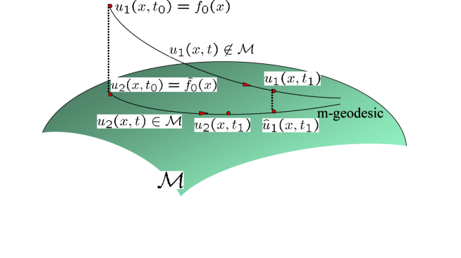
Figure 1: For two solutions $u_{1}(x,t)\not\in{\cal M}$ and $u_{2}(x,t)\in{\cal M}$, the m-projection $\hat{u}_{1}(x,t)$ and $u_{2}(x,t)$ evolve along a common m-geodesic curve on ${\cal M}$ with different velocities.

Next we study the behavior of the solutions $p(x,\tau)$ of the NFPE (2). Recall the transformation from a solution $u(x,t)$ of the PME to $p(x,\tau)$ given in Proposition 4. Since it holds that $dz=(t+1)^{-\alpha}\det(R)dx$, we have the relations of the moments:

$$\int p(z,\tau)dz = \int(t+1)^{\alpha}u(x,t)dz=\det(R)\int u(x,t)dx$$ (31)

$$\int zp(z,\tau)dz = (t+1)^{-\beta}\det(R)R\int xu(x,t)dx$$ (32)

$$\int zz^{T}p(z,\tau)dz = (t+1)^{-2\beta}\det(R)R\left(\int xx^{T}u(x,t)dx\right)R^{T}$$ (33)

The first relation shows that the solution of the NFPE also conserves its mass. Let $\eta^{\rm FP}(\tau)$ and $H^{\rm FP}(\tau)$ be, respectively, the first and second moments of $p(x,\tau)$, i.e.,

$$\eta^{\rm FP}=(\eta_{i}^{\rm FP}),\quad H^{\rm FP}=(\eta_{ij}^{\rm FP}),$$

where

$$\eta_{i}^{\rm FP}:=\mathbf{E}_{p}[x_{i}],\quad\eta_{ij}^{\rm FP}:=\mathbf{E}_{p}[x_{i}x_{j}].$$

From the behavior of the moments of the PME and the above relations, we have

$$\eta^{\rm FP}(\tau) = (t+1)^{-\beta}\det(R)R\eta^{\rm PM}(t)=e^{-\beta\tau}\det(R)R\eta^{\rm PM}(0)$$

$$= e^{-\beta\tau}\eta^{\rm FP}(0),$$

$$H^{\rm FP}(\tau) = (t+1)^{-2\beta}\det(R)RH^{\rm PM}(t)R^{T}$$

$$= e^{-2\beta\tau}\det(R)[RH^{\rm PM}(0)R^{T}+\sigma^{\rm PM}_{u}(e^{\tau}-1)D]$$

$$= e^{-2\beta\tau}H^{\rm FP}(0)+e^{-2\beta\tau}\sigma^{\rm FP}_{p}(e^{\tau}-1)D,$$

where the scaling $\tau=\ln(t+1)$ is assumed and $\sigma^{\rm FP}_{p}(t)$ is defined by

$$\sigma^{\rm FP}_{p}(t) := \det(R)\sigma^{\rm PM}_{u}(t)$$

$$= 2\int_{0}^{\ln(1+t)}d\tau^{\prime}e^{\tau^{\prime}+\alpha(1-m)\tau^{\prime}}\int p(x,\tau^{\prime})^{m}dx$$

for a solution $u$ of the PME and the corresponding solution $p$ of the NFPE. Note that differentiating the above by $t$, we have

$$(1+t)^{\alpha(1-m)}\int p(x,\tau)^{m}dx=\det(R)\int u(x,t)^{m}dx.$$ (34)

For the limiting case $m\rightarrow 1$ (and accordingly $\beta\rightarrow 1/2$), we see that the above expressions recover the well-known linear Fokker-Plank case with a drift vector $x/2$:

$$\eta^{\rm FP}(\tau)=e^{-\tau/2}\eta^{\rm FP}(0),\quad H^{\rm FP}(\tau)=e^{-\tau}H^{\rm FP}(0)+2(1-e^{-\tau})D.$$

Since we know that $p(x,\tau)$ converges to $p_{\infty}(x)\in{\cal M}$ in (26) and it holds that

$$\lim_{\tau\rightarrow\infty}H^{\rm FP}(\tau)=\sqrt{\det D}\left(\lim_{t\rightarrow\infty}(t+1)^{-2\beta}\sigma^{\rm PM}_{u}(t)\right)D$$ (35)

because $\det R=\sqrt{\det D}$, we conclude that the left-hand side of (35) exists and $\sigma^{\rm PM}_{u}(t)=O(t^{2\beta})$ as $t\rightarrow\infty$ (Cf. Remark 2). Summing up the above with Proposition 2, we obtain the following geometric property of the NFPE:

Corollary 2

Consider solutions of the NFPE with the common initial first and second moments. Then their m-projections to ${\cal M}$ evolve along with the common m-geodesic curve from the density determined by the initial moments to the equilibrium $p_{\infty}(x)$.

Note that the following relation holds with the scaling $\tau=\ln(t+1)$:

$$\frac{d}{d\tau}H^{\rm FP}(\tau)=(t+1)^{-2\beta}\left(-2\beta H^{\rm FP}(0)-2\beta\sigma_{u}^{\rm PM}(t)D+(t+1)\frac{d\sigma_{u}^{\rm PM}(t)}{dt}D\right).$$ (36)

Hence, we cannot guarantee the monotonic behavior of the second moment matrix $H^{\rm FP}(\tau)$ unlike the linear Fokker-Planck equation. For example, if the initial density $p(x,0)$ is not on ${\cal M}$ but has the common second moments with the equilibrium density, we cannot expect the right-hand side of (36) is zero and the second moment matrix possibly oscillates around its equilibrium.

3.3 Convergence rate of the solution of the PME to ${\cal M}$

Finally, we show that the triangle equality of the divergence is useful to estimate the convergence rate of the solution of the PME to ${\cal M}$. It is known [14, 15, 17] that a solution of the NFPE decays exponentially with respect to the divergence, i.e.,

$${\cal D}[p(x,\tau)\|p_{\infty}(x)]={\cal F}[p(x,\tau)]-{\cal F}[p_{\infty}(x)]\leq{\cal D}[p(x,0)\|p_{\infty}(x)]e^{-2\beta\tau}.$$ (37)

Proposition 6

Let $u(x,t)$ be a solution of the PME and $\hat{u}(x,t)$ be the m-projection of $u(x,t)$ to the $q$-Gaussian family ${\cal M}$ at each $t$. Then $u(x,t)$ asymptotically approaches ${\cal M}$ satisfying

$${\cal D}[u(x,t)\|\hat{u}(x,t)]\leq\frac{C_{0}}{1+t},$$

where $C_{0}$ is a constant depending on the initial function $u(x,0)$.

Proof) Owing to the triangular equality of the m-projection in Proposition 3, it holds that

$${\cal D}[p(x,\tau)\|\hat{p}(x,\tau)]+{\cal D}[\hat{p}(x,\tau)\|p_{\infty}(x)]={\cal D}[p(x,\tau)\|p_{\infty}(x)].$$

Together with (37), we have

$${\cal D}[p(x,\tau)\|\hat{p}(x,\tau)]\leq{\cal D}[p(x,0)\|p_{\infty}(x)]e^{-2\beta\tau}.$$

Let $u(x,t)$ and $\hat{u}(x,t)$ be functions defined from $p(x,\tau)$ and $\hat{p}(x,\tau)$, respectively, through the transformation in Proposition 4. Then, it is easy to see that $\hat{u}(x,t)\in{\cal M}$ if and only if $\hat{p}(x,\tau)\in{\cal M}$ at each fixed $t$ (and $\tau$). Further, since the first and second moments of $p(x,\tau)$ and $\hat{p}(x,\tau)$ are equal, so are those of $u(x,t)$ and $\hat{u}(x,t)$ from (32) and (33). Thus, we conclude that $\hat{u}(x,t)$ is also the m-projection of $u(x,t)$. It holds from (34) that

$$\det(R)\int\hat{u}(x,t)^{m}-u(x,t)^{m}dx=(1+t)^{\alpha(1-m)}\int\hat{p}(x,\tau)^{m}-p(x,\tau)^{m}dx.$$

Hence, the relation in Remark 1 shows that

$${\cal D}[u(x,t)\|\hat{u}(x,t)] = (1+t)^{\alpha(1-m)}{\cal D}[p(x,\tau)\|\hat{p}(x,\tau)]/\det(R)$$

$$\leq (1+t)^{\alpha(1-m)-2\beta}C_{0}=(1+t)^{-1}C_{0}$$

because $\alpha(1-m)-2\beta=-1$. Q.E.D.

Remark 3

From the above result we can conclude that the $L^{1}$ convergence of $u(x,t)$ to ${\cal M}$ is with the rate $1/\sqrt{1+t}$, using the Csiszar-Kullback inequality [14]. This implies that the convergence to ${\cal M}$ is faster than that to the self-similar solution of the PME (cf. the next subsection), the rate of which is known to be $1/t^{\beta}$ when $1<m\leq 2$ [16, 17]. This might be a new aspect of the convergence properties for solutions of the PME.

3.4 The trajectory of self-similar solution

For the PME (1) there exists a special solution on ${\cal M}$ called the self-similar solution or Barenblatt-Pattle solution [51, 52]. The solution is expressed in terms of the $q$-Gaussian density for the case of unit mass by

$$u^{\rm BP}(x,t) := t^{-\alpha}\left(C-\frac{(m-1)\beta}{2m}t^{-2\beta}x^{T}x\right)^{1/(m-1)}$$ (38)

$$= t^{-\alpha}\exp_{q}\left(t^{-2\beta}x^{T}\Theta(1)x-\psi(0,\Theta(1))\right)$$

$$= \exp_{q}\left(x^{T}\Theta(t)x-\psi(0,\Theta(t))\right)$$

$$= G_{q}(x;0,\Theta(t)),\quad\Theta(t)=-t^{-1}\frac{\beta}{2m}I,$$

where $C$ is a constant for $u^{\rm BP}(x,t)$ to have unit mass and the normalizing constant satisfies

$$\psi(0,\Theta(t))=\frac{1-Ct^{\alpha(1-m)}}{m-1}.$$

The self-similar solution plays an important role in analysis of the PME [16]. It is known that any solution for the PME with unit initial mass converges to $u^{\rm BP}(x,t)$, e.g., in $L^{1}$ norm $\lim_{t\rightarrow\infty}\|u(x,t)-u^{\rm BP}(x,t)\|_{1}=0$ [16, 17]. Geometrically, it is also special in the following sense:

Lemma 1

The trajectory of the self-similar solution $u^{\rm BP}(x,t)$ is a curve on ${\cal M}$ that is simultaneously an m- and e-geodesic.

Proof) In Theorem 1 we have already proved that the trajectory is an m-geodesic. Since (38) shows that the trajectory is expressed as a straight line in the canonical coordinate system $(\theta,\Theta)$, the statement follows from Proposition 2. Q.E.D.

Remark 4

The property of the self-similar solution stated in the above lemma is called doubly autoparallel [53]. From this we can readily conclude that the trajectory of the self-similar solution is also a geodesic with respect to the Levi-Civita connection.

As an application of this property, we have the following decomposition of the divergence:

Proposition 7

Let $u(x,t)$ be a solution of the PME and $\hat{u}(x,t)$ be its m-projection to ${\cal M}$. For the trajectory of the self-similar solution $u^{\rm BP}(x,t)$ with $0<t$ denoted by $\gamma$, define the m-projection of $\hat{u}(x,t)$ to $\gamma$ by

$$u^{*}(x,t):=\arg\min_{r(x)\in\gamma}{\cal D}[\hat{u}(x,t)\|r(x)].$$

Then it holds for all $t>0$ that

$${\cal D}[u(x,t)\|u^{\rm BP}(x,t)] = {\cal D}[u(x,t)\|\hat{u}(x,t)]$$

$$+{\cal D}[\hat{u}(x,t)\|u^{*}(x,t)]+{\cal D}[u^{*}(x,t)\|u^{\rm BP}(x,t)].$$

Proof) From Proposition 3, we have

$${\cal D}[u(x,t)\|u^{\rm BP}(x,t)]={\cal D}[u(x,t)\|\hat{u}(x,t)]+{\cal D}[\hat{u}(x,t)\|u^{\rm BP}(x,t)].$$

The decomposition

$${\cal D}[\hat{u}(x,t)\|u^{\rm BP}(x,t)]={\cal D}[\hat{u}(x,t)\|u^{\rm BP}(x,t)]+{\cal D}[u^{*}(x,t)\|u^{\rm BP}(x,t)]$$

follows from the standard argument of the Pythagorean relation in information geometry [30, 31]. Q.E.D.

4 Conclusions

We have studied the behavior of the solutions to the PME and NFPE focusing on the $q$-Gaussian family ${\cal M}$. By proving that ${\cal M}$ is a stable invariant manifold of the both equations, we have obtained several properties of the solutions, e.g, $N(={\rm dim}{\cal M})$ constants of motions, the convergence rate to ${\cal M}$ and geometrical characterization of the self-similar solution of the PME. In particular, the dependency of the evolutional velocity on the divergence from ${\cal M}$ (Corollary 1) would be a peculiar phenomena to the slow diffusion.

Through the analysis, we see that the generalized concepts of statistical physics and the compatibly defined information geometric structure on ${\cal M}$ provide us with abundant and precise information on the behavior of solutions.

In [15], Otto reported that the PME can be regarded as a gradient system via Riemannian geometry with the Wasserstein metric. The relation with the framework in the present paper is left unclear. Another important future work would be to confirm how the obtained results are analogously extended to the other parameter ranges: $2\leq m$ or $m<1$ (fast diffusion), or the other type of nonlinear diffusion equation.

References

References

- [1] Muskat M 1937 The Flow of Homogeneous Fluids Through Porous Media (New York: McGraw-Hill)
- [2] Buckmaster J 1977 Viscous sheets advancing over dry beds J. Fluid Mech. 81 735–56
- [3] Larsen E W and Pomraning G C 1980 Asymptotic analysis of nonlinear Marshak waves SIAM J. Appl. Math. 39 201–12
- [4] Kath W L 1985 Waiting and propagating fronts in nonlinear diffusion Physica D 12 375–81
- [5] Barenblatt G I 1996 Scaling, self-similarity and intermediate asymptotics (Cambridge: Cambridge Univ. Press)
- [6] Friedman A and Kamin S 1980 The asymptotic behavior of gas in an N-dimensional porous medium Trans. Amer. Math. Soc. 262 551–63
- [7] Aronson D G 1985 The Porous Medium Equation Lecture Notes in Mathematics 1224 (Berlin/New York: Springer-Verlag)
- [8] Newman W 1984 A Lyapunov functional for the evolution of solutions to the porous medium equation to self-similarity I J. of Math. Phys. 25 3124–27
- [9] Ralston J 1984 A Lyapunov functional for the evolution of solutions to the porous medium equation to self-similarity II J. of Math. Phys. 25 3120–23
- [10] Plastino A R and Plastino A 1995 Non-extensive statistical mechanics and generalized Fokker-Planck equation Physica A 222 347–54
- [11] Shiino M 1998 H-theorem with generalized relative entropies and the Tsallis statistics J. Phys. Soc. Jpn. 67 3658–60
- [12] Frank T D 2001 Lyapunov and free energy functionals of generalized Fokker-Planck equations Physics Letters A 290 93–100
- [13] Frank T D 2002 Generalized Fokker-Planck equations derived from generalized linear nonequilibrium thermodynamics Physica A 310 397–412
- [14] Carrillo J A and Toscani G 2000 Asymptotic L1-decay of solutions of the porous medium equation to self-similarity Indiana Univ. Math. J. 49 113–41
- [15] Otto F 2001 The geometry of dissipative evolution equations: the porous medium equation Comm. Partial Differential Equations 26 101–74
- [16] Vázquez J L 2003 Asymptotic behaviour for the porous medium equation posed in the whole space J. Evol. Equ. 3 67–118
- [17] Toscani G 2005 A central limit theorem for solutions of the porous medium equation J. Evol. Equ. 5 185–203
- [18] Frank T D 2005 Nonlinear Fokker-Planck Equations: Fundamentals and Applications (Berlin/Heidelberg: Springer-Verlag)
- [19] Vázquez J L 2006 Smoothing and decay estimates for nonlinear diffusion equations : equations of porous medium type (Oxford: Oxford University)
- [20] Vázquez J L 2007 The porous medium equation: Mathematical theory (Oxford: Oxford University)
- [21] Ambrosio L A, Gigli N and Savaré G 2005 Gradient flows: in metric spaces and in the space of probability measures (Basel: Birkhäuser)
- [22] Carrillo J A, Di Francesco M and Toscani G 2006 Intermediate asymptotics beyond homogeneity and self-similarity: long time behavior for Arch. Ration. Mech. Anal. 180 127–49
- [23] Dolbeault J and del Pino M 2002 Best constants for gagliardo-nirenberg inequalities and application to nonlinear diffusions J. Math. Pures Appl. 81 847–75
- [24] Villani C 2003 Topics in optimal transportation (Providence: American Mathematical Society)
- [25] Carrillo J A, McCann R J and Villani C 2006 Contractions in the 2-Wasserstein Length Space and Thermalization of Granular Media Arch. Ration. Mech. Anal. 179 217–63
- [26] Otto F and Westdickenberg M 2006 Eulerian calculus for the contraction in thewasserstein distance SIAM J. Math. Anal. 37 1227–55
- [27] Villani C 2009 Optimal transport: old and new (Berlin/Heidelberg: Springer-Verlag)
- [28] Tsallis C, Levy S V F, Souza A M C and Maynard R 1995 Statistical-mechanical foundation of the ubiquity of Levy distributions in nature Physical Review Letters 75 3589–93, 1996 Errata, 77 5442
- [29] Suyari H and Tsukada M 2002 Law of errors in Tsallis statistics IEEE Trans. Inf. Theory 51 2, 753–7
- [30] Amari S-I 1985 Differential-Geometrical Methods in Statistics Lecture Notes in Statistics, Vol. 28, (New York: Springer-Verlag)
- [31] Amari S-I and Nagaoka H 2000 Methods of Information Geometry Trans. Math. Mono., Vol.191, (Providence: AMS)
- [32] Eguchi S 2006, Information geometry and statistical pattern recognition Sugaku Expositions 19 197–216, (originally 2004 Sūgaku, 56 380–99 in Japanese.)
- [33] Murata N, Takenouchi T, Kanamori T and Eguchi S 2004 Information geometry of U-Boost and Bregman divergence Neural Computation 16 1437–81
- [34] Naudts J 2002 Deformed exponentials and logarithms in generalized thermodynamics Physica A 316 323–34
- [35] Naudts J 2004 Generalized thermodynamics based on deformed exponentials and logarithmic functions Physica A 340 32-40
- [36] Naudts J 2004 Continuity of a class of entropies and relative entropies, Reviews in Mathematical Physics 16 809–22
- [37] Naudts J 2004 Estimators, escort probabilities, and -exponential families in statistical physics J. Ineq. Pure Appl. Math 5 102
- [38] Burbea J 1986 Informative geometry of probability spaces Expo. Math. 4 347–78
- [39] Mitchell A F S 1989 The information matrix, skewness tensor and -connections for the general multivariate elliptic distribution Ann. Inst. Statist. Math. 41 289–304
- [40] Oller J M and Corcuera J M 1995 Intrinsic analysis of statistical estimation Ann. Stat. 23 1562–81
- [41] Andai A 2008 On the geometry of generalized Gaussian distributions J. Multivariate Anal. 100 777-93
- [42] Grunwald P D and David A P 2004 Game theory, maximum entropy, minimum discrepancy and robust baysian decision theory Annals of Statistics 32 1367–433
- [43] David A P 2007 The geometry of proper scoring rules, Annals of Institute of Statistics 59, 77-93
- [44] Minami M and Eguchi S 2002 Robust blind source separation by beta-divergence Neural Computation 14, 1859-86
- [45] Higuchi I and Eguchi S 2004 Robust principal component analysis with adaptive selection for Tuning Parameters, J. Machine Learning Research 5, 453–71
- [46] Takenouchi T and Eguchi S 2004 Robustifying AdaBoost by adding the naive error rate Neural Computation 16 767–87
- [47] Tsallis C 1988 Possible generalization of Boltzmann-Gibbs statistics, J. Stat. Phys. 52 479–87
- [48] Wada T and A.M.Scarfone A M 2005 Connection between Tsallis’ formalisms employing the standard linear average energy and ones employing the normalized -average energy Physics Letters A 335 351–62
- [49] Callen H B 1985 Thermodynamics and an Introduction to Thermostatistics second ed. (New York: Wiley)
- [50] Ohara A 2009 Geometric study for the Legendre duality of generalized entropies and its application to the porous medium equation, Topical issue on SigmaPhi 2008, European Physical Journal B 70 15-28
- [51] Barenblatt G I 1952 On some unsteady motions of a liquid or a gas in a porous medium Prikl. Mat. Mekh. 16 67-78 (in Russian)
- [52] Pattle R E 1959 Diffusion from an instantaneous point source with concentration dependent coefficient Quart. Jour. Mech. Appl. Math. 12 407–09
- [53] Uohashi K and Ohara A 2004 Jordan Algebras and Dual Affine Connections on Symmetric Cones Positivity 8 369–78