Spherical Deformation for one-dimensional Quantum Systems

Abstract

System-size dependence of the ground-state energy $E^{N}_{~{}}$ is investigated for $N$-site one-dimensional (1D) quantum systems with open boundary condition, where the interaction strength decreases towards the both ends of the system. For the spinless Fermions on the 1D lattice we have considered, it is shown that the finite-size correction to the energy per site, which is defined as $E^{N}_{~{}}\!/N-\lim_{N\rightarrow\infty}^{~{}}E^{N}_{~{}}\!/N$, is of the order of $1/N^{2}_{~{}}$ when the reduction factor of the interaction is expressed by a sinusoidal function. We discuss the origin of this fast convergence from the view point of the spherical geometry.

1 Introduction

A purpose of numerical studies in condensed matter physics is to obtain bulk properties of systems in the thermodynamic limit. In principle numerical methods are applicable to systems with finite degrees of freedom, and therefore occasionally it is impossible to treat infinite system directly. A way of estimating the thermodynamic limit is to study finite-size systems, and subtract the finite-size corrections by means of extrapolation with respect to the system size. [1, 2].

As an example of extensive functions, which is essential for bulk properties, we consider the ground state energy $E^{N}_{~{}}$ of $N$-site one-dimensional (1D) quantum systems. In this article we focus on the convergence of energy per site $E^{N}_{~{}}/N$ with respect to the system size $N$. In order to clarify the discussion, we specify the form of lattice Hamiltonian

$$\hat{H}=\sum_{\ell}^{~{}}\,\hat{h}_{\ell,\ell+1}^{~{}}+\sum_{\ell}^{~{}}\,\hat{g}_{\ell}^{~{}}\,,$$ (1)

which contains on-site terms $\hat{g}_{\ell}^{~{}}$ and nearest neighbor interactions $\hat{h}_{\ell,\ell+1}^{~{}}$. We assume that the operator form of $\hat{h}_{\ell,\ell+1}^{~{}}$ and $\hat{g}_{\ell}^{~{}}$ are independent of the site index $\ell$, which means that $\hat{H}$ is translationally invariant in the infinite $N$ limit. It is possible to include $\hat{g}_{\ell}^{~{}}$ into $\hat{h}_{\ell,\ell+1}^{~{}}$ by the redefinition

$$\hat{h}_{\ell,\ell+1}^{~{}}+\frac{\hat{g}_{\ell}^{~{}}+\hat{g}_{\ell+1}^{~{}}}{2}\,\,\,\,\rightarrow\,\,\,\,\hat{h}_{\ell,\ell+1}^{~{}}\,,$$ (2)

and therefore we group $\hat{g}_{\ell}^{~{}}$ with $\hat{h}_{\ell,\ell+1}^{~{}}$ as shown in Eq. (1$\cdot$2) if it is convenient. A typical example of such $\hat{H}$ is the spin Hamiltonian of the Heisenberg chain

$$\hat{H}=J\,\sum_{\ell}^{~{}}\,\hat{\bf S}_{\ell}^{~{}}\cdot\hat{\bf S}_{\ell+1}^{~{}}-B\,\sum_{\ell}^{~{}}\,\hat{S}_{\ell}^{Z}\,,$$ (3)

where $\hat{\bf S}_{\ell}^{~{}}$ represents the spin operator at $\ell$-th site, and $\hat{S}_{\ell}^{Z}$ its $Z$-component. The parameters $J$ and $B$ are, respectively, the neighboring interaction strength and the external magnetic field. In this case $\hat{h}_{\ell,\ell+1}^{~{}}$ and $\hat{g}_{\ell}^{~{}}$ are, respectively, $J\,\hat{\bf S}_{\ell}^{~{}}\cdot\hat{\bf S}_{\ell+1}^{~{}}$ and $-B\hat{S}_{\ell}^{Z}$. If the chain is infinitely long, $\hat{H}$ in Eq. (1$\cdot$3) is translational invariant, and the ground state $|\Psi_{0}^{~{}}\rangle$ is uniform when there is no symmetry breaking. For example, the bond-energy $J\,\langle\,\hat{\bf S}_{\ell}^{~{}}\cdot\hat{\bf S}_{\ell+1}^{~{}}\rangle=J\,\langle\Psi_{0}^{~{}}|\,\hat{\bf S}_{\ell}^{~{}}\cdot\hat{\bf S}_{\ell+1}^{~{}}\,|\Psi_{0}^{~{}}\rangle$ of the integer-spin Heisenberg chain is independent on $\ell$.

This homogeneous property of the system is violated if only a part of the interactions $\hat{h}_{1,2}^{~{}}$, $\hat{h}_{2,3}^{~{}}$, $\ldots$, and $\hat{h}_{N-1,N}^{~{}}$ is present, and the rest does not exist. In other words, if we consider an $N$-site open boundary system defined by the Hamiltonian

$$\hat{H}_{\rm Open}^{~{}}=\sum_{\ell=1}^{N-1}\,\hat{h}_{\ell,\ell+1}^{~{}}+\sum_{\ell=1}^{N}\,\hat{g}_{\ell}^{~{}}\,,$$ (4)

the ground state $|\Psi_{0}^{~{}}\rangle$ is normally non-uniform. As a result the expectation values $\langle\hat{h}_{\ell,\ell+1}^{~{}}\rangle$ and $\langle\hat{g}_{\ell}^{~{}}\rangle$ are position dependent, especially near the boundary of the system. The ground state energy $E_{~{}}^{N}$ of this $N$-site system is normally not proportional to the system size $N$, which shows the presence of boundary energy correction. Such a finite-size effect is non-trivial when the system is gapless, as observed in the $S=1/2$ Heisenberg spin chain [18].

In case that we are interested in the bulk property of the system, it is better to reduce the boundary effect as rapidly as possible. For this purpose Vekić and White introduced a sort of smoothing factor $A_{\ell}^{~{}}$ to the Hamiltonian

$$\hat{H}_{\rm Smooth}^{~{}}=\sum_{\ell=1}^{N-1}A_{\ell}^{~{}}\,\left(\hat{h}_{\ell,\ell+1}^{~{}}+\frac{\hat{g}_{\ell}^{~{}}+\hat{g}_{\ell+1}^{~{}}}{2}\right)\,,$$ (5)

where $A_{\ell}^{~{}}$ is almost unity deep inside the system and decays to zero near the both boundaries of the system [3]. The factor $A_{\ell}^{~{}}$ is adjusted so that the boundary effect disappears rapidly with respect to the distance from the boundary. A simplest parametrization is to reduce only $A_{1}^{~{}}$ and $A_{N-1}^{~{}}$ from unity, leaving other factors equal to unity. This simple choice of $A_{\ell}^{~{}}$ is often used for calculations of the Haldane gap [4].

As an alternative approach, Ueda and Nishino recently introduced the hyperbolic deformation, which is characterized by the non-uniform Hamiltonian

$$\hat{H}_{\rm Hyp.}^{~{}}=\sum_{\ell=1}^{N-1}\cosh\left(\lambda\,\frac{2\ell-N-1}{2}\right)\,\,\left(\hat{h}_{\ell,\ell+1}^{~{}}+\frac{\hat{g}_{\ell}^{~{}}+\hat{g}_{\ell+1}^{~{}}}{2}\right)\,,$$ (6)

where $\lambda$ is a small positive constant of the order of $0.01\sim 0.1$ [21, 22]. As long as the form of the Hamiltonian is concerned, $\hat{H}_{\rm Hyp.}^{~{}}$ can be regarded as a special case of $\hat{H}_{\rm Smooth}^{~{}}$ in Eq. (1$\cdot$5) with $A_{\ell}^{~{}}=\cosh\left(\lambda\,{\textstyle\frac{2\ell-N-1}{2}}\right)$. But in the scheme of hyperbolic deformation, the factor $\cosh\left(\lambda\,{\textstyle\frac{2\ell-N-1}{2}}\right)$ is an increasing function of $|(2\ell-N-1)/2|$, and therefore the boundary effect is in principle enhanced. This enhancement works uniformly for most of the lattice sites, and the expectation value $\langle h_{\ell,\ell+1}^{~{}}\rangle=\langle\Psi_{0}^{~{}}|\,h_{\ell,\ell+1}^{~{}}\,|\Psi_{0}^{~{}}\rangle$ for the ground state $|\Psi_{0}^{~{}}\rangle$ becomes nearly independent on $\ell$ for most of the bonds. After obtaining the expectation value $\langle h_{\ell,\ell+1}^{~{}}\rangle$ at the center of the system for several values of the deformation parameter $\lambda$, one can perform an extrapolation towards $\lambda=0$ to get the energy per site of the undeformed system. Such an extrapolation is possible since the hyperbolic deformation has an effect of decreasing the correlation length of the system.

The hyperbolically deformed system is closely related to classical lattice models on the hyperbolic plane with a constant and negative curvature. [5, 6, 7, 8, 9, 10, 11, 12, 13, 14, 15, 16] In this article we imagine the case of a positive constant curvature, where the classical lattice models are on a sphere. The corresponding quantum Hamiltonian can be written as

$$\hat{H}_{\rm Sph.}^{~{}}=\sum_{\ell=1}^{N-1}\sin\frac{\ell\pi}{N}\,\left(\hat{h}_{\ell,\ell+1}^{~{}}+\frac{\hat{g}_{\ell}^{~{}}+\hat{g}_{\ell+1}^{~{}}}{2}\right)\,,$$ (7)

where $A_{\ell}^{~{}}=\sin(\ell\pi/N)$ decreases to zero toward the system boundary. We call such a modification of the bond strength as the spherical deformation, and consider $N$ as the system size. We analyze the ground state $|\Psi_{0}^{~{}}\rangle$ and the ground-state energy $E^{N}_{~{}}$ of this deformed Hamiltonian for the case of spinless free Fermions on the lattice. We find that the difference

$$\frac{E^{N}_{~{}}}{N}-\lim_{N\rightarrow\infty}^{~{}}\frac{E^{N}_{~{}}}{N}\,,$$ (8)

which is the finite-size correction included in the energy per site $E^{N}_{~{}}/N$, is of the order of $1/N^{2}_{~{}}$. Note that this $1/N^{2}_{~{}}$ dependence is the same as observed for the system with periodic boundary conditions, described by the Hamiltonian

$$\hat{H}_{\rm Periodic}^{~{}}=\sum_{\ell=1}^{N-1}\left(\hat{h}_{\ell,\ell+1}^{~{}}+\frac{\hat{g}_{\ell}^{~{}}+\hat{g}_{\ell+1}^{~{}}}{2}\right)+\left(\hat{h}_{N,1}^{~{}}+\frac{\hat{g}_{N}^{~{}}+\hat{g}_{1}^{~{}}}{2}\right)\,.$$ (9)

In a certain sense, the spherically deformed system does not contain system boundary.

Structure of this article is as follows. In the next section we introduce a spinless free Fermion model on 1D lattice. For tutorial purpose, the finite-size effect is reviewed for systems with open and periodic boundary conditions. In Sec. 3 we show our numerical results obtained from the diagonalization of the spherically deformed Hamiltonian $\hat{H}_{\rm Sph.}^{~{}}$ in Eq. (1$\cdot$7). In Sec. 4 we consider geometrical meaning of the spherical deformation by way of the Trotter decomposition applied to the deformed Hamiltonian. We also consider a continuous limit, where the lattice spacing becomes zero. We summarize the obtained results in the last section.

2 Energy corrections in the free fermion system

As an example of 1D quantum systems, we consider the spinless free Fermions on the 1D lattice. The Hamiltonian is defined as

$$\hat{H}=-t\,\sum_{\ell}^{~{}}\left(\hat{c}_{\ell}^{\dagger}\hat{c}_{\ell+1}^{~{}}+\hat{c}_{\ell+1}^{\dagger}\hat{c}_{\ell}^{~{}}\right)-\mu\,\sum_{\ell}^{~{}}\hat{c}_{\ell}^{\dagger}\hat{c}_{\ell}^{~{}}\,,$$ (10)

where $t$ and $\mu$ are, respectively, the hopping parameter and the chemical potential. For simplicity we set $\mu=0$ and treat the half-filled state in this Section when $\mu$ is not explicitly shown. As a preparation for the spherical deformation, let us observe the ground state properties of the above Hamiltonian, when open or periodic boundary conditions are imposed for finite-size systems at half filling.

First we consider the $N$-site system with open boundary conditions, where the Hamiltonian is written as

$$\hat{H}^{~{}}_{\rm O}=-t\,\sum_{\ell=1}^{N-1}\left(\hat{c}_{\ell}^{\dagger}\hat{c}_{\ell+1}^{~{}}+\hat{c}_{\ell+1}^{\dagger}\hat{c}_{\ell}^{~{}}\right)\,.$$ (11)

Since there is no interaction, the one-particle eigenstate $|\psi_{m}^{~{}}\rangle$ represented by the wave function

$$\langle 0|\hat{c}_{\ell}^{~{}}|\psi_{m}^{~{}}\rangle=\psi^{~{}}_{m}(\ell)=\sqrt{\frac{2}{N+1}}\,\sin\frac{m\pi\ell}{N+1}$$ (12)

is essential for the ground-state analysis, where $m$ is the integer within the range $1\leq m\leq N$. The corresponding one particle energy is

$$\varepsilon_{m}^{~{}}=-2t\,\cos\frac{m\pi}{N+1}\,,$$ (13)

and the ground-state energy at half filling is obtained by summing up all the negative eigenvalues. Assuming that $N$ is even, the ground-state energy is obtained as

$$E_{\rm O}^{N}=\sum_{m=1}^{N/2}\varepsilon_{m}^{~{}}=t\left[1-\left(\sin\frac{\pi/2}{N+1}\right)^{-1}_{~{}}\right]\,$$ (14)

after a short calculation. Expanding the r.h.s. with respect to $N$, one finds the asymptotic form

$$\frac{E_{\rm O}^{N}}{N}\sim-\frac{2}{\pi}t+\frac{t}{N}\left(\frac{2}{\pi}-1\right)\,.$$ (15)

Compared with the energy per site in the thermodynamic limit

$$\lim_{N\rightarrow\infty}^{~{}}\frac{E_{\rm O}^{N}}{N}=\frac{1}{\pi}\int_{0}^{\pi/2}-2t\,\cos k\,dk=-\frac{2}{\pi}t\,,$$ (16)

it is shown that the finite-size correction to the energy per site (or even to the energy per bond) is of the order of $1/N$.

The $N$-dependence of the energy correction changes if we impose the periodic boundary conditions, where the Hamiltonian is given by

$$\hat{H}^{~{}}_{\rm P}=-t\,\sum_{\ell=1}^{N-1}\left(\hat{c}_{\ell}^{\dagger}\hat{c}_{\ell+1}^{~{}}+\hat{c}_{\ell+1}^{\dagger}\hat{c}_{\ell}^{~{}}\right)-t\left(\hat{c}_{N}^{\dagger}\hat{c}_{1}^{~{}}+\hat{c}_{1}^{\dagger}\hat{c}_{N}^{~{}}\right)\,.$$ (17)

In this case, the one-particle wave function is the plane wave

$$\psi^{~{}}_{m}(\ell)=\sqrt{\frac{1}{N}}\,\exp\left[i\frac{2m\pi(\ell-1)}{N}\right]\,,$$ (18)

where $m$ is an integer that satisfies $-N/2+1<m\leq N/2$. The corresponding one-particle energy is

$$\varepsilon_{m}^{~{}}=-2t\,\cos\frac{2m\pi}{N}\,.$$ (19)

If $N$ is a multiple of four, the ground state energy at half filling is calculated as

$$E_{\rm P}^{N}=\sum_{m=-N/4+1}^{N/4}\varepsilon_{m}^{~{}}=-2t\,\cot\frac{\pi}{N}\,.$$ (20)

Thus, the finite-size correction to the energy per site

$$\frac{E_{\rm P}^{N}}{N}-\left(-\frac{2}{\pi}t\right)=-\frac{2t}{N}\,\cot\frac{\pi}{N}+\frac{2t}{\pi}\,\,\sim\,\,\frac{2\pi t}{3N^{2}_{~{}}}$$ (21)

is of the order of $1/{N^{2}_{~{}}}$.

As verified in the above calculations, the finite-size correction to the energy per site $E^{N}_{~{}}/N$ decreases faster for the system with the periodic boundary conditions than with the open boundary conditions. Regardless of this fact, the open boundary systems are often chosen in numerical studies by the density matrix renormalization group (DMRG) method [18, 17, 19, 20] because of the simplicity in numerical calculation. It should be noted that for those systems that exhibits incommensurate modulation, the open boundary condition is more appropriate than the periodic boundary condition. Thus, it will be convenient if there is a way of decreasing the finite-size correction to $E^{N}_{~{}}/N$ as fast as $1/N^{2}_{~{}}$ also for the open boundary systems.

3 Spherical deformation

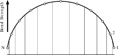
Figure 1: A spherically deformed lattice, which contains $(N\!=\!11)$-sites, drawn on the upper half of the circumference. Open circles denote lattice sites, where the angle of the $\ell$-th site is $\theta_{\ell}^{~{}}=(\ell-\frac{1}{2})\pi/N$ for $\ell=1,\,2,\,\ldots,\,N$. The length of the vertical line shows the relative strength $\sin(\ell\pi/N)$ of the bond drawn by the thick arc between $\ell$-th and $(\ell+1)$-th sites.

We first consider the $N$-site open boundary system described by the Hamiltonian

$$\hat{H}^{~{}}_{\rm S}=-t\,\sum_{\ell=1}^{N-1}\sin\frac{\ell\pi}{N}\,\left(\hat{c}_{\ell}^{\dagger}\hat{c}_{\ell+1}^{~{}}+\hat{c}_{\ell+1}^{\dagger}\hat{c}_{\ell}^{~{}}\right)\,.$$ (22)

Compared with the undeformed Hamiltonian $\hat{H}^{~{}}_{\rm O}$ in Eq. (2$\cdot$2), the strength of the hopping term is scaled by the factor $A_{\ell}^{~{}}=\sin(\ell\pi/N)$, which decreases towards the system boundary as shown in Fig. 1. For a geometrical reason which we discuss in the next section, we call the modification from $\hat{H}^{~{}}_{\rm O}$ to $\hat{H}^{~{}}_{\rm S}$ as the spherical deformation. We regard $N$, the number of sites on the upper half of the circumference shown in Fig. 1, as the system size.

Let us observe the $N$ dependence of the ground-state energy at half filling, where $n_{\ell}^{~{}}=\langle{\hat{c}}_{\ell}^{\dagger}{\hat{c}}_{\ell}^{~{}}\rangle=1/2$ is satisfied by the particle-hole symmetry. So far we have not obtained the analytic form of the one-particle wave function $\psi^{~{}}_{m}$, except for the zero-energy state, and the corresponding one-particle eigenvalue $\varepsilon^{~{}}_{m}$ for the deformed Hamiltonian $\hat{H}_{\rm S}^{~{}}$. We therefore calculate them numerically by diagonalizing $\hat{H}^{~{}}_{\rm S}$ in the one-particle subspace. We then obtain the expectation value $\langle\hat{c}_{\ell}^{\dagger}\hat{c}_{\ell+1}^{~{}}+\hat{c}_{\ell+1}^{\dagger}\hat{c}_{\ell}^{~{}}\rangle$ and the ground state energy $E_{\rm S}^{N}$ at half filling. In the following numerical calculations, we set $t$ as the unit of the energy.

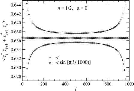
Figure 2: The circles shows the expectation value $\langle\hat{c}_{\ell}^{\dagger}\hat{c}_{\ell+1}^{~{}}+\hat{c}_{\ell+1}^{\dagger}\hat{c}_{\ell}^{~{}}\rangle$ of the spherically deformed lattice Fermion model defined by ${\hat{H}}_{\rm S}^{~{}}$ when $N=1000$. For comparison, we also plot the same expectation value for the undeformed case defined by ${\hat{H}}_{\rm O}^{~{}}$ by the cross marks.

Figure 2 shows $\langle\hat{c}_{\ell}^{\dagger}\hat{c}_{\ell+1}^{~{}}+\hat{c}_{\ell+1}^{\dagger}\hat{c}_{\ell}^{~{}}\rangle$ of the ground state when $N=1000$. For comparison, we also show the same quantity obtained by the undeformed Hamiltonian $\hat{H}^{~{}}_{\rm O}$ of the same system size. As it is observed, the spherical deformation suppresses the position dependence in $\langle\hat{c}_{\ell}^{\dagger}\hat{c}_{\ell+1}^{~{}}+\hat{c}_{\ell+1}^{\dagger}\hat{c}_{\ell}^{~{}}\rangle$. In this sense we can say that the ground state of $\hat{H}^{~{}}_{\rm S}$ is more uniform than that of $\hat{H}^{~{}}_{\rm O}$.

One expects that the ground state energy $E^{N}_{\rm S}$, which is the sum of negative one-particle eigenvalues

$$E^{N}_{\rm S}=\sum_{m=1}^{N/2}\varepsilon^{~{}}_{m}=-t\,\sum_{\ell=1}^{N-1}\sin\frac{\ell\pi}{N}\,\langle\hat{c}_{\ell}^{\dagger}\hat{c}_{\ell+1}^{~{}}+\hat{c}_{\ell+1}^{\dagger}\hat{c}_{\ell}^{~{}}\rangle\,,$$ (23)

is nearly proportional to the sum of the bond strength

$$B^{N}_{~{}}=\sum_{\ell=1}^{N-1}\sin\frac{\ell\pi}{N}=\cot\frac{\pi}{2N}\,.$$ (24)

It is also expected that the ratio $E^{N}_{\rm S}/B^{N}_{~{}}$ rapidly converges to $-2t/\pi$, which is the expectation value $\langle\hat{c}_{\ell}^{\dagger}\hat{c}_{\ell+1}^{~{}}+\hat{c}_{\ell+1}^{\dagger}\hat{c}_{\ell}^{~{}}\rangle$ in the thermodynamic limit. Figure 3 shows $E^{N}_{\rm S}/B^{N}_{~{}}$ and $E^{N}_{\rm P}/N$ with respect to $1/N^{2}_{~{}}$. Obviously, the finite-size corrections $E^{N}_{\rm P}/N+2t/\pi$ and $E^{N}_{\rm S}/B^{N}_{~{}}+2t/\pi$ are nearly proportional to $1/N^{2}_{~{}}$. In order to confirm this $1/N^{2}_{~{}}$ dependence, we show $[E_{\rm P}^{N}/N-E_{\rm S}^{N}/B^{N}_{~{}}]N^{2}_{~{}}$ in Fig. 4, where the value converges to a constant in the limit $N\rightarrow\infty$. Calculating the ratio between $|E^{N}_{\rm P}/N+2t/\pi|$ and $|E^{N}_{\rm S}/B^{N}_{~{}}+2t/\pi|$, we find that the former is twice as large as the latter in the limit $N\rightarrow\infty$. The result suggests that the spherically deformed $N$-site system is related to a system of size $2N$ with periodic boundary conditions.

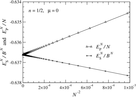
Figure 3: The finite-size corrections to the energy per site at half filling $n=1/2$. Crosses show $E^{N}_{\rm S}/B^{N}_{~{}}$ and the open circles $E^{N}_{\rm P}/N$.

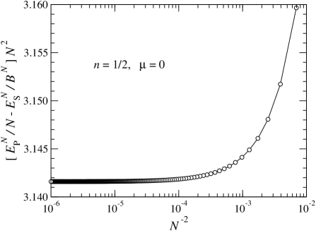
Figure 4: The convergence of $[E_{\rm P}^{N}/N-E_{\rm S}^{N}/B^{N}_{~{}}]N^{2}_{~{}}$ with respect to $1/N^{2}_{~{}}$.

We have considered the half-filled case. Away of the half filling we must include the chemical potential term, which is proportional to $\mu$, into the deformed Hamiltonian. A natural way of introducing $\mu$ is to put it into the bond operator $\hat{h}_{\ell,\ell+1}^{~{}}$, as stated in Eq. (1$\cdot$2). From this extension we obtain the following Hamiltonian

$$\hat{H}^{~{}}_{\rm S}=\sum_{\ell=1}^{N-1}\sin\frac{\ell\pi}{N}\,\left(-t\,\hat{c}_{\ell}^{\dagger}\hat{c}_{\ell+1}^{~{}}-t\,\hat{c}_{\ell+1}^{\dagger}\hat{c}_{\ell}^{~{}}-\mu\frac{\hat{c}_{\ell}^{\dagger}\hat{c}_{\ell}^{~{}}+\hat{c}_{\ell+1}^{\dagger}\hat{c}_{\ell+1}^{~{}}}{2}\right)\,.$$ (25)

It is also possible to introduce the spherical deformation to the on-site terms as

$$\hat{H}^{\prime}_{\rm S}=-t\,\sum_{\ell=1}^{N-1}\sin\frac{\ell\pi}{N}\,\left(\hat{c}_{\ell}^{\dagger}\hat{c}_{\ell+1}^{~{}}+\,\hat{c}_{\ell+1}^{\dagger}\hat{c}_{\ell}^{~{}}\right)-\mu\sum_{\ell=1}^{N}\sin\frac{(\ell-\frac{1}{2})\pi}{N}\,\hat{c}_{\ell}^{\dagger}\hat{c}_{\ell}^{~{}}\,,$$ (26)

according to the height in Fig. 1 at each site. Note that both $\hat{H}^{~{}}_{\rm S}$ in Eq. (3$\cdot$4) and $\hat{H}^{\prime}_{\rm S}$ in Eq. (3$\cdot$5) give the same thermodynamic limit, and that the chemical potential terms do not commute with the kinetic energy in both cases. This is in contrast to the undeformed Hamiltonian

$${\hat{H}}_{\rm O}^{~{}}=-t\,\sum_{\ell=1}^{N-1}\left(\hat{c}_{\ell}^{\dagger}\hat{c}_{\ell+1}^{~{}}+\,\hat{c}_{\ell+1}^{\dagger}\hat{c}_{\ell}^{~{}}\right)-\mu\sum_{\ell=1}^{N}\hat{c}_{\ell}^{\dagger}\hat{c}_{\ell}^{~{}}\,,$$ (27)

where the chemical potential term is proportional to the total number of particles. Since we do not know the analytic formulation of one-particle energy of the deformed Hamiltonians in Eqs. (3$\cdot$4) and (3$\cdot$5), the relation between $\mu$ and the particle filling $n=\sum_{\ell}^{~{}}\langle{\hat{c}}_{\ell}^{\dagger}{\hat{c}}_{\ell}^{~{}}\rangle/N$ is non-trivial. But we are interested in the cases where $N$ is relatively large, therefore it is possible to use the relation $\mu=-2t\,\cos(\pi n)$, which is satisfied by the undeformed Hamiltonian in Eq. (3$\cdot$6) in the limit $N\rightarrow\infty$, as a good approximation for $\mu$ for the spherically deformed system.

Let us observe the occupation $n_{\ell}^{~{}}=\langle\hat{c}_{\ell}^{\dagger}\hat{c}_{\ell}^{~{}}\rangle$ with respect to the position $\ell$ at $1/2$, $1/4$ and $1/8$ fillings, respectively, where the corresponding $\mu$ is $0$, $-2\cos(\pi/4)$, and $-2\cos(\pi/8)$. It is obvious that $n_{\ell}^{~{}}$ is always $1/2$ at half filling, equivalently, when $\mu=0$. Figure 5 shows $n_{\ell}^{~{}}$ calculated for ${\hat{H}}_{\rm S}^{~{}}$ in Eq. (3$\cdot$4) when $N=1000$. The particle distribution is almost uniform, since the ratio of the hopping strength and the chemical potential is independent on the position $\ell$ on the lattice. Figure 6 shows $n_{\ell}^{~{}}$ near the boundary of the system. The oscillations in $n_{\ell}^{~{}}$ decay rapidly with the distance from the boundary. It should be noted that the amplitude of this small oscillation in the particle density decreases with increasing the system size $N$.

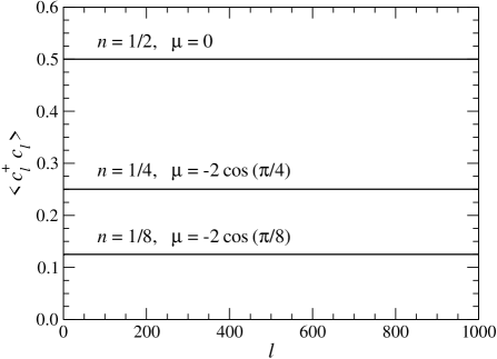
Figure 5: Occupation number $n_{\ell}^{~{}}=\langle\hat{c}_{\ell}^{\dagger}\hat{c}_{\ell}^{~{}}\rangle$ calculated at $1/2$, $1/4$, and $1/8$ filling, respectively, corresponding to the chemical potential $\mu=0$, $-2\cos(\pi/4)$, and $-2\cos(\pi/8)$ for ${\hat{H}}_{\rm S}^{~{}}$ in Eq. (3$\cdot$4).

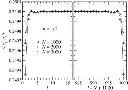
Figure 6: Position dependence in $n_{\ell}^{~{}}=\langle{\hat{c}}_{\ell}^{\dagger}{\hat{c}}_{\ell}^{~{}}\rangle$ near the system boundary at quarter filling.

Figure 7 shows the finite-size correction to the energy per bond at $1/4$ and $1/8$ fillings, calculated for both $H_{\rm S}^{~{}}$ in Eq. (3$\cdot$4) and $H_{\rm S}^{\prime}$ in Eq. (3$\cdot$5). As it is observed at half filling shown in Figs. 3 and 4, the correction is again proportional to $1/N^{2}_{~{}}$. We have thus confirmed the $1/N^{2}_{~{}}$ scaling for the correction to the ground-state energy per site of the spherically deformed lattice-free-Fermion model.

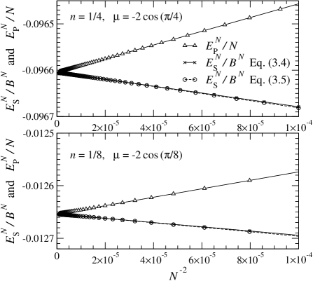
Figure 7: The finite-size corrections to the energy per site, where the crosses show $E^{N}_{\rm S}/B^{N}_{~{}}$ calculated from the Hamiltonian $H_{\rm S}^{~{}}$ Eq. (3.4), the open circles $E^{N}_{\rm S}/B^{N}_{~{}}$ from $H_{\rm S}^{\prime}$ in Eq. (3.5). For comparison we also show the correction $E^{N}_{\rm P}/N$ for the system with periodic boundary conditions by the triangles.

4 Geometrical interpretation

There is a 2D classical system behind a 1D quantum system, where the relation is called as the quantum-classical correspondence. We show that spherically deformed Hamiltonian $\hat{H}_{\rm S}^{~{}}$ corresponds to a classical system on a sphere. We first consider the quantum-classical correspondence by way of the Trotter decomposition [23, 24]. For simplicity we consider the half-filled case ($\mu=0$) for the moment. Let us divide $\hat{H}_{\rm S}^{~{}}$ in Eq. (3$\cdot$4) into two parts

$$\hat{H}_{\rm S}^{~{}}=\sum_{\ell={\rm even}}^{~{}}A_{\ell}^{~{}}\,\hat{h}_{\ell,\ell+1}^{~{}}+\sum_{\ell={\rm odd}}^{~{}}A_{\ell}^{~{}}\,\hat{h}_{\ell,\ell+1}^{~{}}=\hat{H}_{1}^{~{}}+\hat{H}_{2}^{~{}}\,,$$ (28)

where we have used the notation $h_{\ell,\ell+1}^{~{}}=-t\left(\hat{c}_{\ell}^{\dagger}\hat{c}_{\ell+1}^{~{}}+\hat{c}_{\ell+1}^{\dagger}\hat{c}_{\ell}\right)$, and where the deformation factor is given by $A_{\ell}^{~{}}=\sin(\ell\pi/N)$.

The imaginary time evolution of amount of $\beta$ is then expressed by the operator $e^{-\beta\hat{H}_{\rm S}^{~{}}}_{~{}}$. By applying the Trotter decomposition to $e^{-\beta\hat{H}_{\rm S}^{~{}}}_{~{}}$, we obtain

$$e^{-\beta\hat{H}_{\rm S}^{~{}}}_{~{}}=\left(e^{-\beta\hat{H}_{\rm S}^{~{}}/M}_{~{}}\right)^{M}_{~{}}\sim\left(e^{-\beta\hat{H}_{1}^{~{}}/M}_{~{}}\,e^{-\beta\hat{H}_{2}^{~{}}/M}_{~{}}\right)^{M}_{~{}}=\left(e^{-\Delta\beta\hat{H}_{1}^{~{}}}_{~{}}\,e^{-\Delta\beta\hat{H}_{2}^{~{}}}_{~{}}\right)^{M}_{~{}}\,,$$ (29)

where $M$ is the Trotter number [23, 24] and $\Delta\beta=\beta/M$. Looking at the structure of infinitesimal time evolution by $\hat{H}_{1}^{~{}}$

$$e^{-\Delta\beta\hat{H}_{1}^{~{}}}_{~{}}=\exp\left(-\Delta\beta\sum_{\ell={\rm even}}^{~{}}A_{\ell}^{~{}}\,\hat{h}_{\ell,\ell+1}^{~{}}\right)=\exp\left(-\sum_{\ell={\rm even}}^{~{}}\left(\Delta\beta A_{\ell}^{~{}}\right)\,\hat{h}_{\ell,\ell+1}^{~{}}\right)\,,$$ (30)

we find that the quantity

$$\Delta\tau_{\ell}^{~{}}=\Delta\beta\,A_{\ell}^{~{}}$$ (31)

plays the role of the rescaled imaginary time. We can treat $e^{-\Delta\beta\hat{H}_{2}^{~{}}}_{~{}}$ in the same manner. It is possible to interpret $\Delta\tau_{\ell}^{~{}}$ as a kind of proper time [25] at the position $\ell$. Such interpretation leads us to an inhomogeneous time evolution on a (multiply covered) sphere as shown in Fig. 8. This is the reason why we have used the term spherical deformation. Since the surface of the sphere is equivalent everywhere, it is natural to expect that the ground state of the spherically deformed Hamiltonian is approximately uniform.

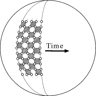
Figure 8: Imaginary time evolution on a sphere.

In the rest of this section we show the correspondence with the spherical geometry by taking the continuous limit to the lattice Hamiltonian $\hat{H}_{\rm S}^{~{}}$ or ${\hat{H}}^{\prime}_{\rm S}$. Consider a 1-particle state

$$|\psi({\tt t})\rangle=\sum_{\ell=1}^{N}\psi_{\ell}^{~{}}({\tt t})\,\hat{c}_{\ell}^{\dagger}|0\rangle$$ (32)

at time ${\tt t}$. (Since we have been using the letter $t$ for the hopping parameter, we use ${\tt t}$ for the time.) The real-time evolution of the wave function $\psi_{\ell}^{~{}}({\tt t})$ is described by the Schrödinger equation

$$i\hbar\frac{\partial}{\partial{\tt t}}\psi_{\ell}^{~{}}=-t\,\sin\frac{\ell\pi}{N}\,\psi_{\ell+1}^{~{}}-t\,\sin\frac{(\ell-1)\pi}{N}\,\psi_{\ell-1}^{~{}}-\mu\sin\frac{(\ell-\frac{1}{2})\pi}{N}\,\psi_{\ell}^{~{}}\,$$ (33)

under the Hamiltonian $\hat{H}_{S}^{\prime}$ in Eq. (3$\cdot$5). Note that the difference between $\hat{H}_{S}^{~{}}$ in Eq. (3$\cdot$4) and $\hat{H}_{S}^{\prime}$ in Eq. (3$\cdot$5) is not relevant in the large $N$ limit. There are two different continuous limits for this spatially discrete Schrödinger equation. We first consider the massive case where $\mu$ is nearly equal to $-2t$. Introducing the notation $f_{\ell}^{~{}}=\sin\left[(\ell-\frac{1}{2})\pi/N\right]$, we can rewrite Eq. (4$\cdot$6) by use of differentials

$$i\hbar\frac{\partial}{\partial{\tt t}}\psi_{\ell}^{~{}} = -t\,f_{\ell+\frac{1}{2}}^{~{}}\,\psi_{\ell+1}^{~{}}-t\,f_{\ell-\frac{1}{2}}^{~{}}\,\psi_{\ell-1}^{~{}}-\mu\,f_{\ell}^{~{}}\,\psi_{\ell}^{~{}}$$

$$= -t\left[f_{\ell+\frac{1}{2}}^{~{}}\left(\psi_{\ell+1}^{~{}}-\psi_{\ell}^{~{}}\right)-f_{\ell-\frac{1}{2}}^{~{}}\left(\psi_{\ell}^{~{}}-\psi_{\ell-1}^{~{}}\right)\right]-\left(\mu\,f_{\ell}^{~{}}+t\,f_{\ell+\frac{1}{2}}^{~{}}+t\,f_{\ell-\frac{1}{2}}^{~{}}\right)\psi_{\ell}^{~{}}\,,$$

where we have substituted the trivial relations $\psi_{\ell+1}^{~{}}=(\psi_{\ell+1}^{~{}}-\psi_{\ell}^{~{}})+\psi_{\ell}^{~{}}$ and $\psi_{\ell-1}^{~{}}=-(\psi_{\ell}^{~{}}-\psi_{\ell-1}^{~{}})+\psi_{\ell}^{~{}}$. Using the relations

$$f_{\ell+\frac{1}{2}}^{~{}} = \frac{1}{2}\left(f_{\ell+\frac{1}{2}}^{~{}}+f_{\ell-\frac{1}{2}}^{~{}}\right)+\left(f_{\ell+\frac{1}{2}}^{~{}}-f_{\ell-\frac{1}{2}}^{~{}}\right)$$

$$f_{\ell-\frac{1}{2}}^{~{}} = \frac{1}{2}\left(f_{\ell+\frac{1}{2}}^{~{}}+f_{\ell-\frac{1}{2}}^{~{}}\right)-\left(f_{\ell+\frac{1}{2}}^{~{}}-f_{\ell-\frac{1}{2}}^{~{}}\right)$$ (35)

we can further rewrite Eq. (4$\cdot$7) as

$$i\hbar\frac{\partial}{\partial{\tt t}}\psi_{\ell}^{~{}}= - \frac{t}{2}\left(f_{\ell+\frac{1}{2}}^{~{}}+f_{\ell-\frac{1}{2}}^{~{}}\right)\left[\left(\psi_{\ell+1}^{~{}}-\psi_{\ell}^{~{}}\right)-\left(\psi_{\ell}^{~{}}-\psi_{\ell-1}^{~{}}\right)\right]$$ (36)

$$- \frac{t}{2}\left(f_{\ell+\frac{1}{2}}^{~{}}-f_{\ell-\frac{1}{2}}^{~{}}\right)\left[\left(\psi_{\ell+1}^{~{}}-\psi_{\ell}^{~{}}\right)+\left(\psi_{\ell}^{~{}}-\psi_{\ell-1}^{~{}}\right)\right]$$

$$- \frac{t}{2}\left(f_{\ell+\frac{1}{2}}^{~{}}+f_{\ell-\frac{1}{2}}^{~{}}\right)2\,\psi_{\ell}^{~{}}-\mu\,f_{\ell}^{~{}}\psi_{\ell}^{~{}}\,.$$

Now we introduce the lattice constant $a=\pi R/N$, where $R$ is the radius of the sphere. We also introduce the spacial co-ordinate $x=a(\ell-\frac{1}{2})$, which satisfies $0<x<\pi R$. Using these notations we rewrite $\psi_{\ell}^{~{}}({\tt t})$ as $\psi(x,{\tt t})$, and $f_{\ell}^{~{}}$ as $f(x)=\sin(x/R)=\sin\theta$, where $\theta=x/R$ is the angle measured from the north pole. The continuous limit can be taken by increasing the number of sites $N$ keeping $R$ constant, where the lattice constant $a$ decreases with $N$. Simultaneously we increase the hopping parameter $t$ so that the relation $a^{2}_{~{}}t=\hbar^{2}_{~{}}/2m$ always holds, where $m$ is the particle mass, and $\hbar$ the Dirac constant. To prevent the divergence in the potential term, we adjust $\mu$ so that $\mu+2t=-V$ is satisfied, where $V$ is a finite constant. Using these parametrizations, we obtain the Schrödinger equation in continuous space

$$i\hbar\frac{\partial}{\partial{\tt t}}\psi(x,{\tt t})=-\frac{\hbar^{2}_{~{}}}{2m}\frac{\partial}{\partial x}\left[f(x)\frac{\partial}{\partial x}\psi(x,{\tt t})\right]+V\,f(x)\psi(x,{\tt t})\,.$$ (37)

This equation is derived from the Lagrangian

$${\cal L}=-i\hbar\,\psi^{*}_{~{}}(x,{\tt t})\frac{\partial}{\partial{\tt t}}\psi(x,{\tt t})+f(x)\left[\frac{\hbar^{2}_{~{}}}{2m}\frac{\partial\psi^{*}_{~{}}(x,{\tt t})}{\partial x}\frac{\partial\psi(x,{\tt t})}{\partial x}+V\psi^{*}_{~{}}(x,{\tt t})\psi(x,{\tt t})\right]\,,$$ (38)

where introduction of proper time $\tau(x,{\tt t})$ that satisfies ${\rm d}{\tt t}=\frac{1}{f(x)}{\rm d}\tau(x,{\tt t})$ draws the following Lagrangian

$${\cal L}=f(x)\left[-i\hbar\,\psi^{*}_{~{}}(x,\tau)\frac{\partial}{\partial\tau}\psi(x,\tau)+\frac{\hbar^{2}_{~{}}}{2m}\frac{\partial\psi^{*}_{~{}}(x,\tau)}{\partial x}\frac{\partial\psi(x,\tau)}{\partial x}+V\psi^{*}_{~{}}(x,\tau)\psi(x,\tau)\right]$$ (39)

in the $x$-$\tau$ space. The action ${\cal S}$ is then written as

$${\cal S}=\int\left[-i\hbar\,\psi^{*}_{~{}}\frac{\partial}{\partial\tau}\psi+\frac{\hbar^{2}_{~{}}}{2m}\frac{\partial\psi^{*}_{~{}}}{\partial x}\frac{\partial\psi}{\partial x}+V\psi^{*}_{~{}}\psi\right]\sin\frac{x}{R}\,\,{\rm d}\tau{\rm d}x\,.$$ (40)

As it is seen, $f(x)\,{\rm d}\tau{\rm d}x=\sin(x/R)\,{\rm d}\tau{\rm d}x$ plays the role of the integral measure on the sphere of radius $R$. Note that the continuous limit for the field operator $\hat{c}_{\ell}^{~{}}\rightarrow\hat{\psi}(x)$ can be taken in the same manner as in Eqs. (4$\cdot$6)-(4$\cdot$13) using the correspondence in Eq. (4$\cdot$5).

Since $f(x)=0$ at the both ends, where $x=0$ and $x=\pi R$, the continuous one-dimensional quantum system in Eqs. (4$\cdot$10)-(4$\cdot$13) does not effectively contain the system boundaries. We can observe the fact by way of the conformal mapping

$$y=-R\,\log\,\cot\left(\frac{x}{2R}\right)$$ (41)

from the sphere embedded in three dimensions onto the infinite plane. We have the relations

$$\sin\frac{x}{R}=2\sin\frac{x}{2R}\cos\frac{x}{2R}=\left(\cosh\frac{y}{R}\right)^{-1}_{~{}}$$ (42)

and $\sin(x/R)\,dy=\sin\theta\,dy=dx$. The action $\cal S$ on this infinite ${\tt t}$-$y$ plane is then written as

$${\cal S}=\int\left[-i\hbar\,\psi^{*}_{~{}}\left(\frac{1}{\sin\theta}\frac{\partial\psi}{\partial{\tt t}}\right)+\frac{\hbar^{2}_{~{}}}{2m}\left(\frac{1}{\sin\theta}\frac{\partial\psi^{*}_{~{}}}{\partial y}\right)\left(\frac{1}{\sin\theta}\frac{\partial\psi}{\partial y}\right)+V\psi^{*}_{~{}}\psi\right]\sin^{2}_{~{}}\theta\,\,{\rm d}{\tt t}{\rm d}y\,,$$ (43)

where $\sin\theta=\left(\cosh\frac{y}{R}\right)^{-1}_{~{}}$ is satisfied. The corresponding one-particle Hamiltonian is obtained as follows

$$H=-\frac{\hbar^{2}_{~{}}}{2m}\frac{\partial}{\partial x}\left(\sin\frac{x}{R}\frac{\partial}{\partial x}\right)+V\,\sin\frac{x}{R}=-\frac{\hbar^{2}_{~{}}}{2m}\cosh\frac{y}{R}\frac{\partial^{2}_{~{}}}{\partial y^{2}_{~{}}}+V\left(\cosh\frac{y}{R}\right)^{-1}_{~{}}\,.$$ (44)

We can also formulate a massless limit, which appears in the case $-2t<\mu<2t$ where there is a Fermi surface, in the same manner as in Eqs. (4$\cdot$6)-(4$\cdot$9). In this case we substitute $\psi_{\ell}^{~{}}=e^{\pm ik\ell}_{~{}}\phi_{\ell}^{~{}}$ to Eq. (4$\cdot$6), where $k$ and $-k$ are, respectively, the Fermi wave number for the right and the left going modes. One finds that the quantity $\nu=at$ is the leading order in the small lattice constant limit $a\rightarrow 0$, equivalently in the large $N$ limit. Adjusting $\mu$ so that $2t\cos k+\mu=-V$ is satisfied, we obtain the equation of motion

$$i\hbar\frac{\partial}{\partial\tt t}\phi(x,{\tt t})=\mp 2i\nu\sin k\frac{\partial}{\partial x}\bigl{[}f(x)\phi(x,{\tt t})\bigr{]}+Vf(x)\phi(x,{\tt t})\,,$$ (45)

for the continuous field $\phi(x,{\tt t})$. The corresponding Lagrangian in $x$-$\tau$ plane is

$${\cal L}=f(x)\left[-i\hbar\,\phi^{*}_{~{}}(x,\tau)\frac{\partial}{\partial\tau}\phi(x,\tau)\pm 2i\nu\sin k\,\phi(x,\tau)\frac{\partial\phi^{*}_{~{}}(x,\tau)}{\partial x}+V\psi^{*}_{~{}}(x,\tau)\psi(x,\tau)\right]\,,$$ (46)

where we have used the fact that $f(0)=f(2R)=0$. Similar to Equations (4$\cdot$13)-(4$\cdot$16), we can consider the conformal mapping for this massless case. The $1/N^{2}_{~{}}$ dependence of the corrections to the ground-state energy per site might be explained by the boundary conformal field theory, where we leave the conjectures for the future study.

5 Conclusions and discussions

We have investigated the ground state of the spherically deformed 1D free Fermion system, for both at the half filling and away of the half filling. The finite-size correction to the energy per site is of the order of $1/N^{2}_{~{}}$ for both cases. The reason for such fast convergence is qualitatively explained by the quantum-classical correspondence, where the spherically deformed Hamiltonians essentially correspond to classical fields on a sphere. In such a sense the spherically deformed system does not contain the system boundary.

Interest in the spherical deformation rests in dynamical properties. We conjecture that a moving one-particle wave packet on the spherically deformed lattice oscillates nearly harmonically as a consequence of the circulation on the sphere. The oscillation may be also explained by a continuous refraction caused by a slower dynamics near the both ends of the system.

As a generalizations of the spherically deformed Hamiltonian ${\hat{H}}_{\rm S}^{~{}}$ in Eq. (1$\cdot$7), one can consider a decoupled Hamiltonian

$$\hat{H}_{\rm sin}^{~{}}=\sum_{\ell=1}^{2N-1}\sin\frac{\ell\pi}{N}\,\left(\hat{h}_{\ell,\ell+1}^{~{}}+\frac{\hat{g}_{\ell}^{~{}}+\hat{g}_{\ell+1}^{~{}}}{2}\right)\,,$$ (47)

where $\ell=2N+1$ is equivalent to $\ell=1$, for a system of size $2N$. The differential with respect to $\ell$ draws

$$\hat{H}_{\rm cos}^{~{}}=\sum_{\ell=1}^{2N-1}\cos\frac{\ell\pi}{N}\,\left(\hat{h}_{\ell,\ell+1}^{~{}}+\frac{\hat{g}_{\ell}^{~{}}+\hat{g}_{\ell+1}^{~{}}}{2}\right)\,,$$ (48)

which is again the decoupled Hamiltonian when $N$ is an even number. [21] Both $\hat{H}_{\rm sin}^{~{}}$ and $\hat{H}_{\rm cos}^{~{}}$ seems to be generators of rotation on a kind of discrete sphere. Their commutation relation would be discussed elsewhere.

If one is interested in the estimation of the excitation gap, the spherical deformation is not appropriate. This is because weak bonds near the system boundary induce spurious low-energy excitations. For this purpose, the hyperbolic deformation is more appropriate [21, 22]. The quantum-classical correspondence discussed in this article can be also considered for the hyperbolic deformation, which would deduce continuous field model on the Poincare disc.

References

[1] M.E Fisher in Proc. Int. School of Physics ‘Enrico Fermi’51
M.S. Green (Ed.) (Academic Press, New York, 1971) 1.
[2] M.N. Barber in Phase Transitions and Critical Phenomena8 (Ed.)
C. Domb and J.L. Lebowitz (Academic Press, New York, 1983) 146.
[3] M. Vekić and S.R. White: Phys. Rev. Lett. 71 (1993) 4283.
[4] S.R. White and D.A. Huse: Phys. Rev. B 48 (1993) 3844.
[5] K. Ueda, R. Krcmar, A. Gendiar, and T. Nishino:
J. Phys. Soc. Jpn. 76 (2007) 084004.
[6] R. Krcmar, A. Gendiar, K. Ueda, and T. Nishino:
J. Phys. A Math. Theor 41 (2008) 215001.
[7] A. Gendiar, R. Krcmar, K. Ueda, and T. Nishino:
Phys. Rev. E 77 (2008) 041123.
[8] S.K. Baek, P. Minnhagen, and B.J. Kim:
Europhys. Lett. 79 (2007), 26002.
[9] F. Sausset and G. Tarjus: J. Phys. A 40 (2007) 12873.
[10] J.C. Anglés d’Auriac, R. Mélin, P. Chandra, and B. Douçot:
J. Phys. A 34 (2001), 675.
[11] N. Madras and C. Chris Wu:
Combinatorics, Probab., Comput. 14 (2005), 523.
[12] C. Chris Wu: J. Stat. Phys. 100 (2000), 893.
[13] H. Shima and Y. Sakaniwa: J. Phys. A 39 (2006), 4921.
[14] I. Hasegawa, Y. Sakaniwa, and H. Shima: Surface Science 601 (2007), 5232.
[15] R. Rietman, B. Nienhuis, and J. Oitmaa:
J. Phys. A 25 (1992), 6577.
[16] B. Doyon and P. Fonseca: J. Stat. Mech. (2004) P07002.
[17] S.R. White: Phys. Rev. Lett. 69 (1992) 2863.
[18] S.R. White: Phys. Rev. B 48 (1993) 10345.
[19] I. Peschel, X. Wang, M. Kaulke, and K. Hallberg (Eds.)
(Springer Berlin, 1999) Lecture Notes in Physics 528‘Density-Matrix Renormalization, A New Numerical Method in Physics’
[20] U. Schollwöck: Rev. Mod. Phys. 77 (2005) 259.
[21] H. Ueda and T. Nishino: J. Phys. Soc. Jpn. 78 (2008) 014001.
[22] H. Ueda and T. Nishino: arXiv/0812.4513.
[23] H.F. Trotter: Proc. Am. Math. Soc. 10 (1959) 545.
[24] M. Suzuki: Prog. Theor. Phys. 56 (1976) 1454.
[25] Note that we are considering an infinitesimal time evolution, and
we do not consider the global geodesics that starts from the position on the
discretized sphere.