Numerical simulation of stochastic motion of vortex loops under action
of random force. Evidence of the thermodynamic equilibrium.

Abstract

Numerical simulation of stochastic dynamics of vortex filaments under action of random (Langevin) force is fulfilled. Calculations are performed on base of the full Biot–Savart law for different intensities of the Langevin force. A new algorithm, which is based on consideration of crossing lines, is used for vortex reconnection procedure. After some transient period the vortex tangle develops into the stationary state characterizing by the developed fluctuations of various physical quantities, such as total length, energy etc. We tested this state to learn whether or not it the thermodynamic equilibrium is reached. With the use of a special treatment, so called method of weighted histograms, we process the distribution energy of the vortex system. The results obtained demonstrate that the thermodynamical equilibrium state with the temperature obtained from the fluctuation dissipation theorem is really reached.
PACS-numbers: 67.40.Vs 98.80.Cq 7.37.+q

I Introduction

Quantized vortices appeared in quantum fluids and other systems play a fundamental role in the properties of the latter. For that reason they have been an object of intensive study for many years (for review and bibliography see e.g. Don ). The greatest success in investigations of dynamics of quantized vortices has been achieved in relatively simple cases such as a vortex array in rotating helium or vortex rings. However these simple cases are rather exception than a rule. Due to extremely involved dynamics initially straight lines or rings evolve to form highly entangled chaotic structure. Thus, the necessity of statistic methods to describe chaotic vortex loop configurations arises. A most tempting way is to treat vortices as a kind of excitations and to use thermodynamic methods. One of first examples of that way was an use the Landau criterium for critical velocity where vortex energy and momentum were applied to relation having pure thermodynamic sense. More extended examples would be the famous Kosterlitz–Thouless theory or its 3D variant intensively being developed currently {for review and bibliography see e.g. Williams ). In the examples above and in many other it is assumed that chaotic vortex configuration is in thermal equilibrium and their statistics obeys the Gibbs distribution. That belief is based on fundamental physical principles and can be justified in a standard way considering vortex loops as a subsystem submerged into thermostat and exchanging with energy with the latter. However numerous experiments on counterflowing HeII, and direct numerical simulations of vortex line dynamics Don , NF , Chorin94 convincingly demonstrate that this dynamics is essentially nonequilibrium and possesses all features inherent in turbulent phenomena. Thus a question arises how a thermal equilibrium is destroyed and what mechanisms are responsible for that. To answer that question we have firstly to understand in details how a thermal equilibrium in vortex loop configuration space is established. A general principle of maximum entropy does not give any details the dynamic details are absorbed by a temperature definition. It is well known however that the Gibbs distribution can be alternatively obtained on the basis of some reduced model like kinetic equations or Fokker–Planck equation (FPE). That way of course is not of such great generality as a principle of maximum entropy, but instead it allows to clarify the mechanisms how the Gibbs distribution established nemirTMF .

In the presented paper we report preliminary results of numerical study on dynamics of vortex tangle under action of random (Langevin) forcing delta correlated both in space and time. The data obtained were tested to learn whether or not the stationary state reached in numerical experiment is the thermodynamical equilibrium state. With use a special treatment, so called method of weighted histograms, to process distribution energy of the vortex system. The results obtained demonstrated that the thermodynamical equilibrium with the temperature obtained from the the fluctuation dissipation theorem is really reached.

II The Numerical Simulation and Results

We consider the dynamics of vortex loops in three-dimensional space with no boundaries. The equation of motion of the vortex line elements is supposed to be:

$$\dot{\mathbf{s}}=\dot{\mathbf{s}}_{B}+\alpha(\mathbf{s^{\prime}\times(v}_{n}\mathbf{-\dot{s}}_{B}\mathbf{))-}\alpha\mathbf{{}^{\prime}s^{\prime}\times[s^{\prime}\times(v}_{n}\mathbf{-\dot{s}}_{B}\mathbf{)]+f(}\xi,t\mathbf{),\quad\quad\quad\quad\quad}$$ (1)

where $\dot{\mathbf{s}}_{B}$ is the propagation velocity of the vortex filament at a point $\mathbf{s}$, defined by Biot-Savart low; $\mathbf{s(\xi,t)}$ is the radius-vector of the vortex line points; $\mathbf{v}_{n}$ is the normal velocity of the superfluid helium; $\xi$ is a label parameter, in this case it the arc length; $\mathbf{s^{\prime}}$ is the derivative wrt the arc length, $\alpha$, $\alpha^{\prime}$ are the friction coefficients, describing interaction of vortex filament with normal component, and $\mathbf{f(}\xi,t\mathbf{)}$ is the Langevin force. Further we will take $\mathbf{v}_{n}=0$ and neglect the term with $\alpha^{\prime}$. The Langevin force is supposed to be a white noise with the following correlator

$$\left\langle\mathbf{f}_{i}(\xi_{1},t_{1})\mathbf{f}_{j}(\xi_{2},t_{2})\right\rangle\ =D\delta_{ij}\delta\ (t_{1}-t_{2})\delta\ (\xi_{1}-\xi_{2}).$$ (2)

Here $i,j$ are the spatial components; $t_{1},t_{2}$ are the arbitrary time moments; $\xi_{1},\xi_{2}$ define any points on the vortex line; $D$ is the intensity of the Langevin’s force. Let us consider the probability distribution functional nemirTMF defined as

$$\mathcal{P}(\{\mathbf{s}(\xi)\},t)=\left\langle\delta\left(\mathbf{s}(\xi)-\mathbf{s}(\xi,t)\right)\right\rangle.$$ (3)

The Fokker-Planck equation for the time evolution of quantity $\mathcal{P}(\{\mathbf{s}(\xi)\},t)$ can be derived from equation of motion (1) in standard way (see e.g. Zinn-Justin96 ,nemirTMF )

$$\frac{\partial\mathcal{P}}{\partial t}+\int d\xi\frac{\delta}{\delta\mathbf{s}(\xi)}\left[\dot{\mathbf{s}}_{B}+\alpha\mathbf{s}^{\prime}(\xi)\times\dot{\mathbf{s}}_{B}\right]\mathcal{P}+$$ (4)

$$\int\int d\xi d\xi^{\prime}\left\langle\mathbf{f(}\xi\mathbf{)f(}\xi^{\prime})\right\rangle\delta(\xi\mathbf{-}\xi^{\prime})~{}\delta(t_{1}-t_{2})~{}\delta_{\eta_{1},\eta_{2}}~{}\frac{\delta}{\delta\mathbf{s}(\xi)}\frac{\delta}{\delta\mathbf{s}(\xi^{\prime})}\mathcal{P}=0.$$

As it was shown in nemirTMF the Fokker-Planck equation (4) has a stationary solution

$$\mathcal{P}(\{\mathbf{s}(\xi)\},t)=\exp(-H\left\{\mathbf{s}\right\}/k_{B}T).$$ (5)

Here $H\left\{\mathbf{s}\right\}$ is the hamiltonian - the energy of the vortex system expressed via the whole line configuration

$$H\left\{\mathbf{s}\right\}=E=\int\frac{{\rho}_{s}\mathbf{v}_{s}^{2}}{2}\;d^{3}\mathbf{r}=\frac{\rho_{s}\kappa^{2}}{8\pi}\int\limits_{0}^{L}\int\limits_{0}^{L^{\prime}}\frac{(d\mathbf{s}_{1}d\mathbf{s}_{2})}{|\mathbf{s}_{1}-\mathbf{s}_{2}|}.$$ (6)

The “ temperature” $T$ enterring equation (4) is determined with the help of the fluctuation dissipation theorem

$$\left\langle\mathbf{f}_{\eta_{1}}\mathbf{(}\xi_{1},t_{1})~{}\mathbf{f}_{\eta_{2}}\mathbf{(}\xi_{2},t_{2})\right\rangle~{}=\frac{k_{B}T\alpha}{\rho_{s}\pi(\hbar/m)}~{}\delta(\xi_{1}\mathbf{-}\xi_{2})~{}\delta(t_{1}-t_{2})~{}\delta_{\eta_{1},\eta_{2}}.$$ (7)

In discrete variant of parametrization of the curve, used in numerical simulation, the delta function $~{}\delta(\xi_{1}\mathbf{-}\xi_{2})$ is changed with $1/a$, where $a$ is the step along the curve. Thus intensity $D$ of pumping external Langevin force is connected to the “ temperature” via relation

$$D=2kTa/(\rho_{s}\kappa).$$ (8)

Thus, we demonstated that the set of filament agitating by the random white noise is driven into thermodynamical equilibrium with the temperature relating to intensity of the random forcing. The main purpose of the the present work is to demonstrate it in the direct numerical simulation.

Details of numerical simulation were described in our early publication K04 . The new algorithm for vortex reconnection processes basing on the consideration of crossing lines is used . We run the calculations with $\alpha=0.098$, $D_{1}=9.8\cdot 10^{-5}$ cm²/s, $D_{2}=10.2\cdot 10^{-5}$ cm² /s. In our calculations we start with an initial vortex configuration of twenty four vortex rings (see Fig. 1 (a)). The initial condition was chosen to make the total momentum of the system is equal to zero.

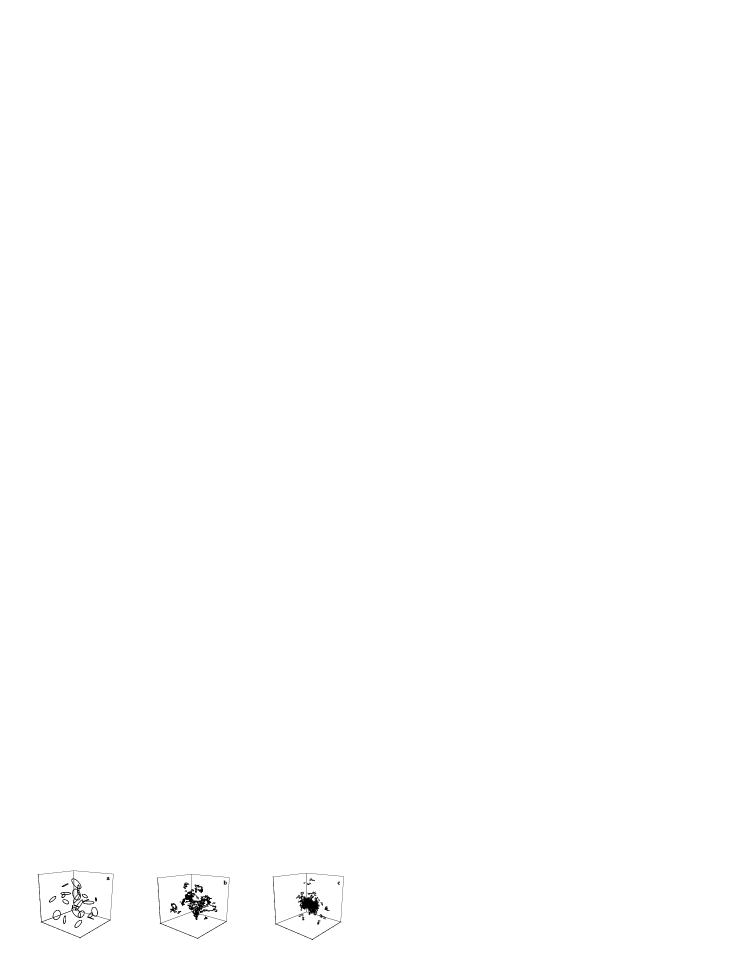
Figure 1: Development of a vortex tangle: t = 0 ($a$) , $t=6$ ($b$), $t=120$ ($c$) ms.

To check the behavior of the system we had been monitoring the total length of the vortex tangle. These quantities for two different intensities of the random forcing were plotted as functions of time in Fig. 2. One can see, at the beginning the total length rapidly increases. When the vortex tangle becomes dense enough many small vortex loops appear due to reconnection processes (see Fig.1(b)). These small loops are radiated in the ambient space and the total length decrease. Finally a stationary state with the strongly fluctuating is achieved see Fig.1 (c). We aim now to study this steady state and give some proofs it be in thermal equilibrium. We use for it the the weighted histogram analysis method, widely used in the Monte Carlo computer simulations of the Ising model F88 .

Figure 2: The lengths of lines as a function of time for different intensity of the Langevin’s force $D$.

To apply the weighted histogram analysis method we take for every run $N$ configurations of the vortex tangle at $\ N$ different moments in time. We supposed these configurations to be statistically independent. We calculate  further (With the use of relation (6)) the energies of the every configurations. Dividing then the whole interval of energies in pieces of width $\Delta E$ we build up the histograms showing relative frequency of meeting the configuration with the energies lying in the interval between $E_{j}$ and $E_{j}+\Delta E$ (see Fig.3). Let us introduce the probability density $P(E_{j})$ of the observing the vortex system state with the energies lying in the interval between $E_{j}$ and $E_{j}+\Delta E.$ Obviously, the $P(E_{j})$ can be simply counted  from histogams with the following relation

$$P(E_{j})=N(E_{j})/(N\Delta E).$$ (9)

Here $N(E_{j})$ is the number of states in the interval between $E_{j}$ and $E_{j}+\Delta E$, $N=\sum\limits_{j}N(E_{j})$ is the full number of configurations (for each of two different intensities of the Langevin’s force $D$ ).

Figure 3: Probability density distributions for different intensities of the Langevin’s force $D$ which are approximated by Gaussian curves.

Consequently assuming that the vortex loops system is in the thermal equilibrium we propose that the histograms depicted in Fig.3 can be describes as well with the use of the Gibbs distribution:

$$P(E_{j})=\frac{g(E_{j})e^{-E_{j}/k_{B}T}}{\sum\limits_{j}g(E_{j})e^{-E_{j}/k_{B}T}},$$ (10)

where $g(E_{j})$ is the density of states, and $T$ is the temperature (either $T_{1}$ or $T_{2}$ for each of the runs), calculated from the fluctuation dissipation theorem (7),(8) for different intensities of the Langevin’s force $D_{1}$, $D_{2}$ correspondingly. Relation (10) included the density of states $g(E_{j})$, which is not only known but even is not defined well for set of continious curves. This problem however can be eliminated with the trick offered in paper F88 . Indeed, it is possible to prove that the probability density distribution at $T_{2}$ can be expressed in terms of the distribution at $T_{1}$ in the following way:

$$\tilde{P}_{T_{2}}(E_{j})=\frac{P_{T_{1}}(E_{j})e^{-(\frac{E_{j}}{k_{B}T_{1}}-\frac{E_{j}}{k_{B}T_{2}})}}{\Delta E\sum\limits_{j}P_{T_{1}}(E_{j})e^{-(\frac{E_{j}}{k_{B}T_{1}}-\frac{E_{j}}{k_{B}T_{2}})}}.$$ (11)

Using relation (11) we calculated the probability density $\tilde{P}_{T_{2}}(E_{j})$ for the temperature $T_{2}$ via the probability density $P_{T_{1}}(E_{j})$ and the compared the result obtained with the initial histogram for the $P_{T_{2}}(E_{j})$. At this point there appeared one difficulty. We mentioned that the discrete variant of the fluctuation dissipation theorem we have to change the delta function $~{}\delta(\xi_{1}\mathbf{-}\xi_{2})$ with quantity $1/a$, where $a$ is the step along the curve.  But during evolution the distance between points does not preserves, the elements of line either shrink or stretch. We nontheless retain the initial value of the space step in the definition of the temperature but introduce the fitting parameter for it. As a fitting parameter we taken half as much again the maximum step along the vortex line using in calculation of dynamics of vortex loops. The curves calculated according to equations (9)  (for the temperature $T_{2}$) and (11) are shown in Fig. 4. As it can seen the curves are very close to each other. It means that the ensemble of vortex filaments is driven into thermodynamical equilibrium state.

Figure 4: Probability density distributions at the temperature $T_{2}$: 1 - the curve calculated according to equation (7); 2 - the curve calculated according to equation (8).

As well it is known that in a thermal equilibrium the variance in the energy (or ‘energy fluctuation‘) is connected with the temperature in the following way :

$$\delta E^{2}=Ck_{B}T^{2},$$ (12)

were

$$\delta E^{2}=\left\langle(E-\left\langle E\right\rangle)^{2}\right\rangle,$$ (13)

$C=(\left\langle E_{2}\right\rangle-\left\langle E_{1}\right\rangle)/(T_{2}-T_{1})$ is the heat capacity. We determined energy fluctuations according to equation (12): $\delta E(T_{1})=2.55\cdot 10^{-16}$ J, $\delta E(T_{2})=2.65\cdot 10^{-16}$ J, as well as according to equation  (13): $\delta E(T_{1})=2.30\cdot 10^{-16}$ J, $\delta E(T_{2})=2.87\cdot 10^{-16}$ J. Obtained energy fluctuations are close to each other. It corroborate that the ensemble of vortex filaments is driven into thermodynamical equilibrium state too.

III Conclusion

Grounding on results of theoretical study made by one of the authors we propose that the vortex tangle filaments undergoing the random “ white noise” forcing  is driven into thermodynamical equilibrium state. The temperature of the vortex system determined by the fluctuation dissipation theorem. With the direct numerical simulation we present the proofs of our supposition. The proof was based on the observation that the distribution of the energy satisfied to the Gibbs law. It was shown with the method of weighted histograms, widely used approach in statistical physics.

References

- (1) Donnelly, R.J. Quantized Vortices in Helium II, Cambridge University Press, 1991.
- (2) G.A.Williams, Vortex-Loop Phase Transitions in Liquid Helium, Cosmic Strings, and High-Tc Superconductors, Phys.Rev.Lett., 1999, 82, N6, 1201.
- (3) S. K. Nemirovskii and W. Fiszdon, Chaotic quantized vortices and hydrodynamic processess superfluid helium, Rev. Mod. Phys., 1995, 67, N1, 37.
- (4) A. Chorin, Voticity and Turbulence, Springer-Verlag, New-Yourk, 1994.
- (5) S.K. Nemirovskii, Thermodynamic equilibrium in the system of chaotic quantized vortices in a weakly imperfect Bose gas, Teoretical and Matematical Physics, 2004, 141, N 1, 141.
- (6) Jean Zinn-Justin, Quantum Field Theory and Critical Phenomena, Claberson Press, Oxford, 1992.
- (7) L.P. Kondaurova and S.K. Nemirovskii, Full Biot-Savart numerical simulation of vortices in He II, J. Low Temperature Physics, 2005, 138, N3/4, 555.
- (8) Alan M. Ferrenberg and Robert H. Swendsen, New Monte Carlo technique for studying phase transitions, Phys. Rev. Lett., 1988, 61, 2635.