Ground-State Entropy of the Random Vertex-Cover Problem

Abstract

Counting the number of ground states for a spin-glass or NP-complete combinatorial optimization problem is even more difficult than the already hard task of finding a single ground state. In this paper the entropy of minimum vertex-covers of random graphs is estimated through a set of iterative equations based on the cavity method of statistical mechanics. During the iteration both the cavity entropy contributions and cavity magnetizations for each vertex are updated. This approach overcomes the difficulty of iterative divergence encountered in the zero temperature first-step replica-symmetry-breaking (1RSB) spin-glass theory. It is still applicable when the 1RSB mean-field theory is no longer stable. The method can be extended to compute the entropies of ground-states and metastable minimal-energy states for other random-graph spin-glass systems.

A combinatorial optimization (CO) problem is defined by an energy function $E(\vec{\sigma})$ on configurations $\vec{\sigma}=(\sigma_{1},\sigma_{2},\ldots,\sigma_{N})$ of a $N$-dimensional space, where each variable $\sigma_{i}$ has only a finite number of states (e.g., $\sigma_{i}=\pm 1$). For CO problems in the non-deterministic polynomial-complete (NP-complete) class, searching for configurations of energy equal or very close to the lowest possible value is in general a very difficult task. Statistical physicists relate this computational hardness to the emergence of complex structures in the problem’s configuration space and the proliferation of metastable macroscopic states (macrostates). The entropy spectrum (number of configurations at each minimal-energy level) gives a characterization of the energy landscape of a hard CO problem. Using the first-step replica-symmetry-breaking (1RSB) cavity method of spin-glass theory Mézard and Parisi (2001, 2003); Mézard et al. (2002), the ground-state energy densities for several hard CO problems on random graphs have been calculated with high precision (see, e.g., Refs. Mézard and Parisi (2003); Weigt and Zhou (2006); Mézard and Tarzia (2007)). But estimating the ground-state entropy and the entropies of metastable states is still a challenging theoretical and computational issue.

In the 1RSB cavity approach, the ground-state energy $E^{0}$ of a hard CO problem is evaluated by first assuming the configuration space of the system can be clustered into many macrostates. A variable $i$ experiences in each macrostate an integer-valued field $h_{i}$. The distribution of this field among all the macrostates, $P_{i}(h_{i})$, is then obtained through an iterative numerical scheme Mézard and Parisi (2003). To calculate the ground-state entropy, a conventional technique is to introduce a temperature $T$ and expand the field $h_{i}$ to first order in $T$ at the limit $T\rightarrow 0$ Zdeborová and Mézard (2006):

$$h_{i}=m_{i}+Tr_{i}\ ,$$ (1)

with $m_{i}$ being an integer and $r_{i}$ a finite real value. A set of iterative equations are derived to obtain the joint distribution $P_{i}(m_{i},r_{i})$ of the values $m_{i}$ and $r_{i}$ for each variable $i$. The ground-state entropy $S^{0}$ is then the first order term in the free energy expansion $F(T)=E^{0}-TS^{0}$. This approach works for some relatively simple problems (e.g., graph-matching whose configuration space is ergodic Zdeborová and Mézard (2006), random $Q$-coloring and $K$-SAT which have zero ground-state energy Mézard et al. (2005); Krzakala et al. (2007); Montanari et al. (2008)) but it fails for many other NP-complete CO problems, for which the ground-state energy $E^{0}$ is positive and the $T\rightarrow 0$ 1RSB cavity equations are not stable. For these later systems, at $T=0$ the field $h_{i}$ is not necessarily an integer and the correction $r_{i}$ in Eq. (1) usually diverges at the $T\rightarrow 0$ limit. Consequently, although the $T\rightarrow 0$ 1RSB cavity method is able to estimate the ground-state energy of a hard CO problem with high accuracy (as only the value of $m_{i}$ but not that of $r_{i}$ is used), it often reports a negative or divergent ground-state entropy.

In this paper we use a different way to estimate the ground-state entropy of a CO problem or a finite-connectivity spin-glass. We work directly at temperature zero and, within the 1RSB cavity framework, calculate both the cavity magnetizations and cavity entropies of each variable in each macrostate. A very small cutoff $\epsilon$ is naturally introduced in the iteration of cavity magnetizations to avoid divergence in the iteration of cavity entropies. This approach gives good results when tested on the random vertex-cover problem, the random $3$-SAT problem, and the random $\pm J$ spin-glass model, even when the $T\rightarrow 0$ 1RSB mean-field spin-glass theory is no longer stable. It is also able to calculate the entropies for other minimal-energy levels. Here we focus on the vertex-cover problem (a prototypical NP-hard problem Hartmann and Weigt (2003)) to demonstrate the main ideas of this method. Detailed calculations on other model systems will be reported elsewhere.

Let us first briefly introduce the vertex-cover problem Weigt and Hartmann (2000, 2001). A graph ${\mathcal{G}}$ contains $N$ vertices and $M$ edges. Each edge $(i,j)$ is between a pair of vertices $i,j$. The mean connectivity of the graph is $c=2M/N$, which is the number of edges a vertex on average is connected to. A vertex cover $C$ for graph ${\mathcal{G}}$ contains a subset of vertices of ${\mathcal{G}}$ such that for each edge $(i,j)\in{\mathcal{G}}$, at least one of its extremities is in $C$. If a vertex $i$ is contained in a vertex-cover $C$, we say it is covered in $C$. The energy of a vertex-cover $C$ is defined as its cardinality, $E(C)=|C|$. Graph ${\mathcal{G}}$ has many vertex covers, with energy ranging from the maximum value $N$ to the minimum value $E^{0}_{{\mathcal{G}}}=\min_{C}|C|$. We denote by ${\mathcal{C}}^{0}_{{\mathcal{G}}}$ the set of minimum vertex covers (MVCs) of graph ${\mathcal{G}}$: ${\mathcal{C}}^{0}_{{\mathcal{G}}}=\{C:|C|=E^{0}_{{\mathcal{G}}}\}$. To determine exactly the energy $E^{0}$ of MVCs for a graph in general is a very hard computational problem; to count the number of MVCs is even harder. Using the cavity method of statistical mechanics, the mean energy density of MVCs for random graphs has been evaluated in Refs. Weigt and Hartmann (2000); Zhou (2005); Weigt and Zhou (2006). The entropy of MVCs for a random graph was also estimated by computer simulations Weigt and Hartmann (2001). This work complements Ref. Weigt and Hartmann (2001) by giving an analytical estimation of the ground-state entropy $S^{0}_{{\mathcal{G}}}\equiv\log|{\mathcal{C}}^{0}_{{\mathcal{G}}}|$.

We denote by $\pi_{i}$ the probability of a vertex $i$ being contained in the MVCs,

$$\pi_{i}=\frac{1}{|{\mathcal{C}}^{0}_{{\mathcal{G}}}|}\sum\limits_{C\in{\mathcal{C}}^{0}_{\mathcal{G}}}\mathbb{I}(i\in C)\ ,$$ (2)

where $\mathbb{I}$ is the indicator function. Similar to $\pi_{i}$, for a vertex $j\in\partial i$ (the set of vertices which are connected to $i$ by an edge), we denote by $\pi_{j|i}$ its probability of being in the MVCs of the cavity graph ${\mathcal{G}\backslash i}$ (which is obtained from ${\mathcal{G}}$ by removing vertex $i$ and all its edges).

We consider here the ensemble of random graphs with mean connectivity $c$. When the graph size $N$ is sufficiently large the length of a loop in the graph is of order $\log_{c}(N)$, and a random graph ${\mathcal{G}}$ is locally tree-like. Consider the set $\partial i$ of vertices in the neighborhood of a randomly chosen vertex $i$. If the edges between $i$ and these vertices are deleted, in the cavity graph ${\mathcal{G}\backslash i}$ the shortest length between any two vertices $j,k\in\partial i$ diverges logarithmically with $N$. As a first step, it is therefore assumed that these vertices are uncorrelated in the cavity graph ${\mathcal{G}\backslash i}$, and the probability of finding these vertices in a MVC of ${\mathcal{G}\backslash i}$ can be expressed in a factorized form:

$$\mathbb{P}\bigl{(}\partial i\subset C:C\in{\mathcal{C}}^{0}_{{\mathcal{G}\backslash i}}\bigr{)}=\prod\limits_{j\in i}\pi_{j|i}\ .$$ (3)

Equation (3) is called the Bethe-Peierls approximation and the corresponding cavity method is referred to be replica-symmetric (RS). Under this assumption, the energy and entropy of MVCs for a random graph ${\mathcal{G}}$ can be expressed as Weigt and Zhou (2006)

$$E^{0}_{\mathcal{G}} = \sum\limits_{i}\Delta E_{i}-\sum\limits_{(i,j)}\Delta E_{(i,j)}\ ,$$ (4)

$$S^{0}_{\mathcal{G}} = \sum\limits_{i}\Delta S_{i}-\sum\limits_{(i,j)}\Delta S_{(i,j)}\ ,$$ (5)

where $\Delta E_{x}$ and $\Delta S_{x}$ are, respectively, the contribution to the system’s ground-state energy and entropy from an vertex ($x=i$) or an edge ($x=(i,j)$). For example, $\Delta E_{i}=E^{0}_{\mathcal{G}}-E^{0}_{{\mathcal{G}\backslash i}}$ and $\Delta S_{i}=\log|{\mathcal{C}}^{0}_{\mathcal{G}}|-\log|{\mathcal{C}}^{0}_{{\mathcal{G}\backslash i}}|$.

We shall distinguish three situations when writing down the expressions for $\Delta E_{i}$ and $\Delta S_{i}$. The total number of MVCs of cavity graph ${\mathcal{G}\backslash i}$ which contain the set $\partial i$ is $|{\mathcal{C}}^{0}_{{\mathcal{G}\backslash i}}|\prod_{j\in\partial i}\pi_{j|i}$. This number is positive if all the cavity probabilities $\pi_{j|i}>0$. In this case, when vertex $i$ is added, it will not be in any MVC of ${\mathcal{G}}$ but the set $\partial i$ will be contained in every MVC of ${\mathcal{G}}$. Then we have $\pi_{i}=0$ (vertex $i$ is always non-covered), $\Delta E_{i}=0$, and $|{\mathcal{C}}^{0}_{\mathcal{G}}|=|{\mathcal{C}}^{0}_{{\mathcal{G}\backslash i}}|\prod_{j\in\partial i}\pi_{j|i}$, and the change in entropy is $\Delta S_{i}=\sum_{j\in i}\log\pi_{j|i}$. On the other hand, if in the set $\partial i$ there are at least two vertices which are not in any MVCs of cavity graph ${\mathcal{G}\backslash i}$, then vertex $i$ will be present in all the MVCs of graph ${\mathcal{G}}$. Adding vertex $i$ to a MVC of cavity graph ${\mathcal{G}\backslash i}$ results in a MVC of graph ${\mathcal{G}}$ ($|{\mathcal{C}}^{0}_{\mathcal{G}}|=|{\mathcal{C}}^{0}_{{\mathcal{G}\backslash i}}|$). In this case $\pi_{i}=1$ ($i$ is always covered), $\Delta E_{i}=1$, and $\Delta S_{i}=0$.

Now we consider the remaining case, namely in the set $\partial i$ there is only one vertex (say $j$) which is not in any MVC of graph ${\mathcal{G}\backslash i}$. In this case, each MVC of graph ${\mathcal{G}}$ contains either vertex $i$ or vertex $j$ but not both. The energy increase is $\Delta E_{i}=1$, and the total number of MVCs for graph ${\mathcal{G}}$ is

$$|{\mathcal{C}}^{0}_{\mathcal{G}}|=|{\mathcal{C}}^{0}_{{\mathcal{G}\backslash i}}|+|{\mathcal{C}}^{0}_{{\mathcal{G}}\backslash i,j}|\prod\limits_{k\in\partial i\backslash j}\pi_{k|i}\ ,$$ (6)

where ${\mathcal{C}}^{0}_{{\mathcal{G}}\backslash i,j}$ is the complete set of MVCs for the cavity graph ${\mathcal{G}}\backslash i,j$ (the remaining graph after further removing vertex $j$ from ${\mathcal{G}\backslash i}$), and $\partial i\backslash j$ is the set of direct neighbors except $j$ of vertex $i$. The first term on the right hand side of the equality in Eq. (6) is the number of MVCs which contain vertex $i$, while the second term is the number of MVCs which contain $j$. In this case vertex $i$ is said to be unfrozen. The entropy change $\Delta S_{i}=\log\bigr{(}1+e^{-\Delta S_{j|i}}\prod_{k\in\partial i\backslash j}\pi_{k|i}\bigr{)}$, and $\pi_{i}=1/\bigl{(}1+e^{-\Delta S_{j|i}}\prod_{k\in\partial i\backslash j}\pi_{k|i}\bigr{)}$, where $\Delta S_{j|i}=\log|{\mathcal{C}}^{0}_{{\mathcal{G}\backslash i}}|-\log|{\mathcal{C}}^{0}_{{\mathcal{G}}\backslash i,j}|$ is the entropy change due to adding vertex $j$ to the cavity graph ${\mathcal{G}}\backslash i,j$. We refer $\Delta S_{j|i}$ as a cavity entropy of vertex $j$. Notice that in this case, to properly calculate $\Delta S_{i}$, one needs not only to consider all the MVCs of cavity graph ${\mathcal{G}\backslash i}$ but also vertex-covers with a higher energy $E^{0}_{{\mathcal{G}\backslash i}}+1$.

The energy and entropy contribution of an edge $(i,j)$ can also be obtained similarly. If at least one of the cavity probabilities $\pi_{j|i}$ and $\pi_{i|j}$ is positive, then $\Delta E_{(i,j)}=0$ and $\Delta S_{(i,j)}=\log\bigl{(}1-(1-\pi_{i|j})(1-\pi_{j|i})\bigr{)}$. On the other hand, if both $\pi_{i|j}$ and $\pi_{j|i}$ are zero, then $\Delta E_{(i,j)}=1$ and $\Delta S_{(i,j)}=\log(e^{-\Delta S_{i|j}}+e^{-\Delta S_{j|i}})$.

On each of the $2M$ directed edges $j\rightarrow i$ of graph ${\mathcal{G}}$ there is a cavity probability $\pi_{j|i}$ and a cavity entropy $\Delta S_{j|i}$. After all these $4M$ values are determined, the total ground-state energy and entropy can then be evaluated using Eqs. (4) and (5). Starting from a random initial condition, the values of $\pi_{j|i}$, $\Delta S_{j|i}$, and the cavity energy increase $\Delta E_{j|i}$ can be determined by the following iterative algorithm. Consider vertices $k$ in the neighborhood $\partial j\backslash i$ of a vertex $j$:

1. If all $\pi_{k|j}>0$, then $\pi_{j|i}=0$, $\Delta E_{j|i}=0$, $\Delta S_{j|i}=\sum_{k\in\partial j\backslash i}\log\pi_{k|j}$.

2. If two or more $\pi_{k|j}=0$, then $\pi_{j|i}=1$, $\Delta E_{j|i}=1$, $\Delta S_{j|i}=0$.

3. If only one $\pi_{k|j}=0$, then $\Delta E_{j|i}=1$, and

   $$\pi_{j|i} = \Bigl{(}1+e^{-\Delta S_{k|j}}\prod_{l\in\partial j\backslash i,k}\pi_{l|j}\Bigr{)}^{-1}\ ,$$ (7)

   $$\Delta S_{j|i} = \log\Bigl{(}1+e^{-\Delta S_{k|j}}\prod_{l\in\partial j\backslash i,k}\pi_{l|j}\Bigr{)}\ .$$ (8)

When using Eq. (7) to update the cavity probability $\pi_{j|i}$, sometimes $\pi_{j|i}$ becomes extremely close to zero. A cutoff $\epsilon$ is therefore introduced in the numerical scheme: If the obtained value of $\pi_{j|i}$ is less than $\epsilon$ we set $\pi_{j|i}=0$. The theoretical entropy values shown in Fig. 1 are obtained by setting a cutoff value of $\epsilon=10^{-10}$ (more discussions on the choice of $\epsilon$ are mentioned below).

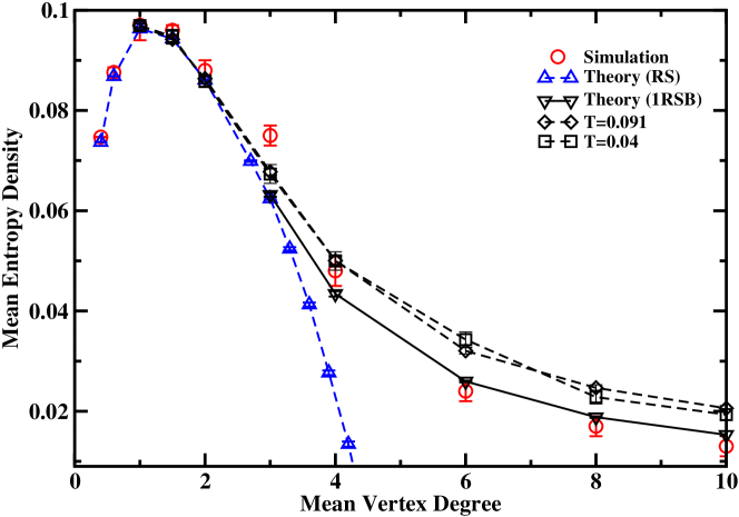
Figure 1: (Color Online) Ground-state entropy density of the vertex-cover problem as a function of the mean vertex degree $c$ of the random graph. Circles are simulation data Weigt and Hartmann (2000), up- and down-triangles are, respectively, theoretical results obtained by the replica-symmetric and the 1RSB cavity method. The finite-temperature entropy density values at $T=0.091$ and $0.04$ are also shown as a comparison.

The above discussion concerns with one large graph ${\mathcal{G}}$. As we are interested in the graph-averaged values for the ground-state energy and entropy, a population dynamics simulation can be performed similarly by storing a large array of $\pi_{j|i}$ and $\Delta S_{j|i}$ and then updating this array Mézard and Parisi (2001); Weigt and Zhou (2006). The ground-state entropy density $s^{0}=\lim_{N\rightarrow\infty}S_{\mathcal{G}}^{0}/N$ as a function of mean connectivity $c$ of the random graph ${\mathcal{G}}$ is evaluated by this numerical scheme (Fig. 1, up-triangles). The ground-state entropy first increases with $c$ and reaches a maximum at $c\approx 1$, then it decreases with $c$. For $c<2.7183$ the RS cavity method is known to be valid Zhou (2005); Weigt and Zhou (2006) and it correctly predicts the ground-state entropy and energy density for the system. For $c>2.7183$ however, the RS prediction is systematically lower than the simulation result of Hartmann and Weigt (circles in Fig. 1) and even becomes negative for $c>4.4$ (such an entropy crisis was also observed in the hitting set problem Mézard and Tarzia (2007)). For $c>2.7183$ the entropy predicted by the RS cavity method depends strongly on the cutoff $\epsilon$. If a smaller $\epsilon$ value is used, the entropy decreases even faster with the mean connectivity $c$.

When the mean connectivity $c$ of the random graph is larger than $2.7183$, the Bethe-Peierls approximation Eq. (3) is no longer a good assumption, as there are strong long-range correlations among distant vertices Zhou (2005). For example, consider two vertices $i$ and $j$ whose shortest-path length is of order $\log_{c}N$ and suppose these two vertices both are unfrozen ($\pi_{i}>0,\pi_{j}>0$) among the space of MVCs of graph ${\mathcal{G}}$. The Bethe-Peierls approximation assumes that the probability of finding a MVC which contains both $i$ and $j$ is equal to $\pi_{i}\pi_{j}>0$. However, it may be the case that there is not a single MVC in which both $i$ and $j$ are present Zhou (2005). To take into account such long-range correlations, in the 1RSB cavity theory the MVC set ${\mathcal{C}}^{0}_{\mathcal{G}}$ of a graph ${\mathcal{G}}$ is clustered into many subsets ${\mathcal{C}}^{0,\alpha}_{\mathcal{G}}$ which are indexed by an index $\alpha$. In each such subset it is assumed that the Bethe-Peierls approximation still holds, and Eq. (3) is replaced by

$$\mathbb{P}\bigl{(}\partial i\subset C:C\in{\mathcal{C}}^{0,\alpha}_{{\mathcal{G}\backslash i}}\bigr{)}=\prod\limits_{j\in i}\pi_{j|i}^{\alpha}\ .$$ (9)

where $\pi_{j|i}^{\alpha}$ is the probability of vertex $j$ being in the MVCs of the $\alpha$-th subset ${\mathcal{C}}^{0,\alpha}_{\mathcal{G}\backslash i}$ of the cavity graph ${\mathcal{G}\backslash i}$. Because of Eq. (9), the iterative equations for $\pi_{j|i}$ and $\Delta S_{j|i}$ as mentioned before are still valid in each subset of MVCs. To characterize the property of different clusters, a probability distribution $\mathcal{P}_{j|i}(\pi,s)$ is introduced on each directed edge of the graph, which is equal to the fraction of MVC clusters with $\pi_{j|i}=\pi$ and $\Delta S_{j|i}=s$. For a single graph ${\mathcal{G}}$ these $2M$ probability distributions $\mathcal{P}_{j|i}$ can again be obtained by iterations, and the corresponding distribution of $\mathcal{P}_{j|i}(\pi,s)$ among all the edges of the random graph can be obtained by mean-field population dynamics.

The iteration equation for $\mathcal{P}_{j|i}(\pi,s)$ reads

$$\mathcal{P}_{j|i}(\pi,s) \propto \int\prod\limits_{k\in\partial j\backslash i}\int{\rm d}\pi_{k|j}{\rm d}s_{k|j}\mathcal{P}_{k|j}(\pi_{k|j},s_{k|j})$$ (10)

$$e^{-y\Delta E_{j|i}}\delta(\pi-\pi_{j|i})\delta(s-\Delta S_{j|i})\ .$$

The value of the re-weighting parameter $y$ in the above equation is chosen such that a complexity parameter is equal to zero Mézard and Parisi (2003). In writing down Eq. (10), it is further assumed that the joint probability of observing the cavity values $(\pi_{k|j},\Delta S_{k|j}),(\pi_{l|j},\Delta S_{l|j}),\ldots$ for vertices $k,l,\ldots\in\partial j\backslash i$ can be written in a factorized form:

$$\mathbb{P}\bigl{(}\pi_{k|j},\Delta S_{k|j};\ldots\bigr{)}=\prod\limits_{m\in\partial j\backslash i}\mathcal{P}_{m|j}(\pi_{m|j},\Delta S_{m|j})\ .$$ (11)

Details of the 1RSB numerical iteration scheme for the vertex-cover problem can be found in Ref. Weigt and Zhou (2006).

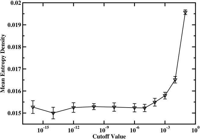
Figure 2: Predicted mean ground-state entropy of the random vertex-cover problem at connectivity $c=10$ as a function of the cutoff parameter $\epsilon$.

The mean entropy density of MVCs for random graphs of mean connectivity $c$ as obtained by this 1RSB cavity method is shown in Fig. 1 (down-triangles). The theoretical predictions are in good agreement with simulation results Weigt and Hartmann (2001). The mean ground-state energy density as obtained by the present method is also in good agreement with the simulation and theoretical results of Ref. Weigt and Zhou (2006). In the calculation we have used a cutoff value $\epsilon=10^{-10}$. Such a cutoff is necessary for the random vertex-cover problem, as the 1RSB cavity approach is not stable to further steps of replica-symmetry-breaking Zhou et al. (2007). Figure 2 shows that, the predicted value of the mean ground-state entropy density is not sensitive to the cutoff parameter $\epsilon$ when $\epsilon\leq 10^{-5}$.

We also carry out lengthy population dynamics simulations at finite temperatures using different protocols. The entropy values obtained at $T=0.091$ and $T=0.04$ are shown in Fig. 1. At these low temperatures although the obtained energy density values are almost indiscernible from the ground-state values, there is still a gap between the finite-temperature and the ground-state entropy density when $c>2.7183$. If further lowering the temperature, the quality of the simulation results deteriorate, possibly because of insufficient population size and insufficient equilibrium and sampling times. We were also unable to remove this gap by using instead the expansion Eq. (1), because the population dynamics diverges. In comparison with these, the zero-temperature direct method is computationally much efficient and also easier to implement.

In summary, we have calculated the ground-state entropy for the random vertex-cover problem using the 1RSB cavity approach of spin-glass theory. In our method, both the cavity probabilities $\pi_{j|i}$ and cavity entropies $\Delta S_{j|i}$ of each vertex $j$ in a cluster of MVC solutions are recorded. We have paid special attention on unfrozen vertices (each of which belongs to some but not all MVCs of the graph). As demonstrated by Eq. (6), the entropy contribution of an unfrozen $i$ comes not only from the MVCs of the graph ${\mathcal{G}\backslash i}$ but also form other higher-energy configurations of ${\mathcal{G}\backslash i}$. Similarly the cavity entropy $\Delta S_{j|i}$ of a vertex $j$ also has two sources of contributions. Equation (6) is rather simple for the vertex-cover problem, while for some other NP-hard CO problems and spin-glass models (e.g., the random-graph $\pm J$ spin-glass) counting the entropy contribution of an unfrozen vertex can be more complicated. A cutoff parameter $\epsilon$ is introduced so that if $\pi_{j|i}<\epsilon$ in one cluster, it is set to be zero. With this cutoff parameter, the present cavity method can still give good estimations on the ground-state entropy of a hard CO problem or spin-glass system even if more steps of replica-symmetry-breaking are needed to fully describe the system.

We thank Alexander Hartmann and Martin Weigt for sharing their simulation data, Pan Zhang for helpful discussions, and KITPC (Beijing) and NORDITA (Stockholm) for hospitality. This work was partially supported by NSFC (Grant No. 10774150).

References

- Mézard and Parisi (2001) M. Mézard and G. Parisi, Eur. Phys. J. B 20, 217 (2001).
- Mézard and Parisi (2003) M. Mézard and G. Parisi, J. Stat. Phys. 111, 1 (2003).
- Mézard et al. (2002) M. Mézard, G. Parisi, and R. Zecchina, Science 297, 812 (2002).
- Weigt and Zhou (2006) M. Weigt and H. Zhou, Phys. Rev. E 74, 046110 (2006).
- Mézard and Tarzia (2007) M. Mézard and M. Tarzia, Phys. Rev. E 76, 041124 (2007).
- Zdeborová and Mézard (2006) L. Zdeborová and M. Mézard, J. Stat. Mech.: Theo. Exp., P05003 (2006).
- Mézard et al. (2005) M. Mézard, M. Palassini, and O. Rivoire, Phys. Rev. Lett. 95, 200202 (2005).
- Krzakala et al. (2007) F. Krzakala, A. Montanari, F. Ricci-Tersenghi, G. Semerjian, and L. Zdeborova, Proc. Natl. Acad. Sci. USA 104, 10318 (2007).
- Montanari et al. (2008) A. Montanari, F. Ricci-Tersenghi, and G. Semerjian, J. Stat. Mech.: Theor. Exper., P04004 (2008).
- Hartmann and Weigt (2003) A. K. Hartmann and M. Weigt, J. Phys. A: Math. Gen. 36, 11069 (2003).
- Weigt and Hartmann (2000) M. Weigt and A. K. Hartmann, Phys. Rev. Lett. 84, 6118 (2000).
- Weigt and Hartmann (2001) M. Weigt and A. K. Hartmann, Phys. Rev. E 63, 056127 (2001).
- Zhou (2005) H. Zhou, Phys. Rev. Lett. 94, 217203 (2005).
- Zhou et al. (2007) J. Zhou, H. Ma, and H. Zhou, J. Stat. Mech.: Theor. Exp., L06001 (2007).