Dynamical Opacity-Sampling Models of Mira Variables. I: Modelling Description and Analysis of Approximations.

Abstract

We describe the Cool Opacity-sampling Dynamic EXtended (CODEX) atmosphere models of Mira variable stars, and examine in detail the physical and numerical approximations that go in to the model creation. The CODEX atmospheric models are obtained by computing the temperature and the chemical and radiative states of the atmospheric layers, assuming gas pressure and velocity profiles from Mira pulsation models, which extend from near the H-burning shell to the outer layers of the atmosphere. Although the code uses the approximation of Local Thermodynamic Equilibrium (LTE) and a grey approximation in the dynamical atmosphere code, many key observable quantities, such as infrared diameters and low-resolution spectra, are predicted robustly in spite of these approximations. We show that in visible light, radiation from Mira variables is dominated by fluorescence scattering processes, and that the LTE approximation likely under-predicts visible-band fluxes by a factor of two.

1 Introduction

Mira-type variable stars represent the last easily observable stage in the evolution of solar-mass stars. Due to the interactions between pulsation, shocks, complex chemistry and radiation pressure, the environment between the continuum-forming photosphere and the dusty wind is complex and difficult to model. For this reason, it has not been possible to extract fundamental parameters of Mira variables (e.g. mass, metallicity and mass-loss rate) from their spectra and light curves alone. Similarly, there are many easily observable properties of Mira variables (such as their visible light curves) that have yet to be put in a firm theoretical context. This is in contrast to Cepheid and RR Lyrae variables, where non-linear effects observable in their light curves have been used to derive accurate (but model-dependent) masses and distances (Keller & Wood, 2006; Marconi & Clementini, 2005).

Furthermore, there has been little detailed theoretical work on the regions of M-type Mira atmospheres between the continuum forming photosphere and the radii approximately 10 times more distant where standard (Draine & Lee, 1984) dust types are stable. These layers are particularly crucial for understanding the interaction between pulsation and mass loss for Mira variables (Wood, 1979; Bowen, 1988; Höfner et al., 1998).

There is a small set of models from other groups that include the effects of interior pulsation by introducing an artificial piston at the base of the atmosphere, although luminosity variations at this position are ignored. These calculations have produced physically consistent dynamical models of the photosphere combined with self-consistent chemical equilibrium calculations and radiative transfer. For C-type Mira variables, this kind of literature is most extensive, with the paper series beginning with Höfner et al. (1998) now including a full treatment of homogeneous nucleation and non-grey radiative transfer as part of the 1-D dynamical atmosphere code.

For M-type Mira variables, models are faced with a more complex chemistry and dust formation, and at least for Miras with periods less than about 500 days, chaotic motions of the atmosphere play a larger role in dynamics than the winds resulting from radiative acceleration of dust grains. Several approaches have been attempted. The models of Höfner et al. (2003) use a non-grey radiative transfer in their dynamical models with mean opacities in 51 frequency meshes, do not consider the formation of dust grains in detail and have not yet been compared with observations. The models of Jeong et al. (2003) use a grey approximation for molecular opacities and a composition-independent dust opacity, but have a sophisticated treatment of the dust nucleation processes. This approach is more applicable to the longer period very dusty Mira variable they modelled than to the more common Miras with periods less than 500 days.

There are no 3-D models of Mira variables at this time, but 2-D models of C-rich Mira variables by Woitke (2006) show the key properties of the shock-dominated dynamics: chaos over large spatial scales similar to the cycle-to-cycle variations seen in 1-D models, and fine structure in the shock fronts caused by the Rayleigh-Taylor instability.

The models in this paper are an improvement on the Hofmann et al. (1998) modelling scheme. Those models were one-dimensional and were based on a three-step modelling process to optimize computational efficiency. First, a grey dynamical model was constructed in which pulsation was self-excited: i.e. there was no ‘piston’ artificially causing the pulsation, and luminosity variations arising in the interior were accounted for. Second, a non-grey radiative transfer scheme was used to calculated the detailed temperature profile of the atmosphere. Finally, more detailed integration through the final atmospheric profile enabled spectra and center-to-limb profiles to be calculated.

Here we describe our Cool Opacity-sampling Dynamic EXtended (CODEX) atmospheric model series for M-type (oxygen-rich) Mira variables. The models include self-excited pulsation with new approximations for convective energy transport (Keller & Wood, 2006), and an opacity-sampling method for radiative transfer in LTE. These models are described in detail in Section 2. They are tested first in Section 3 by further calculations that examine the errors in the approximations caused by our three-step modelling process, and some exploratory calculations into the effects of the LTE approximation and the effect of the dynamical atmosphere (i.e. velocity stratification) on the radiative transfer. The models are further tested in Section 4 by comparison with spectroscopy and optical interferometry, with the aim of determining which model predictions are expected to be most reliable.

2 Modelling Assumptions and Methods

2.1 The pulsation models

The aim of the pulsation models was to produce a Mira model with a period of close to 330 days, which matches the period of the local Mira variable $o$ Ceti. The near-infrared JHK photometry of Whitelock et al. (2000), combined with the distance estimate of 107 pc to $o$ Ceti from the Hipparcos parallax (Knapp et al., 2003) or the LMC ($M_{\rm bol}$, $\log P$) relation for a 330 day Mira variable (Hughes & Wood, 1990; Feast et al., 1989), yields a mean luminosity of close to 5400 L_⊙. This mean luminosity was adopted for the model: giving it the name o54. Given the luminosity, the luminosity-core mass relation (e.g Wood & Zarro, 1981) defines the mass of the core (0.568 M_⊙) below the inner boundary of the pulsating envelope, which is set at about 10⁷ K and a radius of 0.3 R_⊙. A mass of 1.1 M_⊙ was adopted, to match the mass estimated from Galactic kinematics for a Mira of period $\sim$330 days (Jura & Kleinmann, 1992). A metal abundance Z = 0.02 was adopted, along with a helium abundance Y=0.3, which is close to the envelope helium abundance of a 1.1 M_⊙ star on the AGB after it has undergone first and second dredge-up (Bressan et al., 1993).

The self-excited pulsation models were made with the pulsation code described in Keller & Wood (2006). Given the physical input parameters above, and adopted values of the model parameters $\alpha_{m}$ (mixing-length in units of pressure scale heights) and $\alpha_{\nu}$ (the turbulent viscosity parameter) the model naturally pulsates, with the amplitude limited by the non-linear loss processes of shocks in the outer atmosphere and turbulent viscosity. After beginning with a static model, the nonlinear pulsation model was run to limiting amplitude. The period of this model was then compared to the desired period of 330 days, and the amplitude was compared to the observed pulsation amplitude (from the photometry of Whitelock et al . 2000). The value of $\alpha_{m}$ was then adjusted until the correct period was obtained, and $\alpha_{\nu}$ was adjusted to give the correct pulsation amplitude. The final values adopted were $\alpha_{m}$ = 3.5 and $\alpha_{\nu}$ = 0.25. The static model of the so-called parent star with 5400 L_⊙ has a photospheric radius $R_{p}$ = 215 R_⊙ and an effective temperature $T_{\rm eff}$ = 3380 K. The pulsation period of this model in the linear approximation was 330 days.

The long-term behavior of these models is illustrated in Figure 1. The shaded regions are the phases chosen for input into the more detailed atmospheric models. In this paper we only consider models from the third shaded region (between $\sim$7000 and 8000 days), which we label the fx series of models.

The grey radiative transfer in the outer layers of these models is based on Rosseland opacities of Rogers & Iglesias (1992) and Ferguson et al. (2005). In the outer atmosphere, the simple ad-hoc modification of the radiative diffusion equation at small optical depths used by Fox & Wood (1982) is adopted. This approximation guarantees $T\propto r^{-0.5}$ in the outer layers. However, this approach is not accurate enough for spectrum computation, so we choose to re-solve for the gas temperature, as described in the following section.

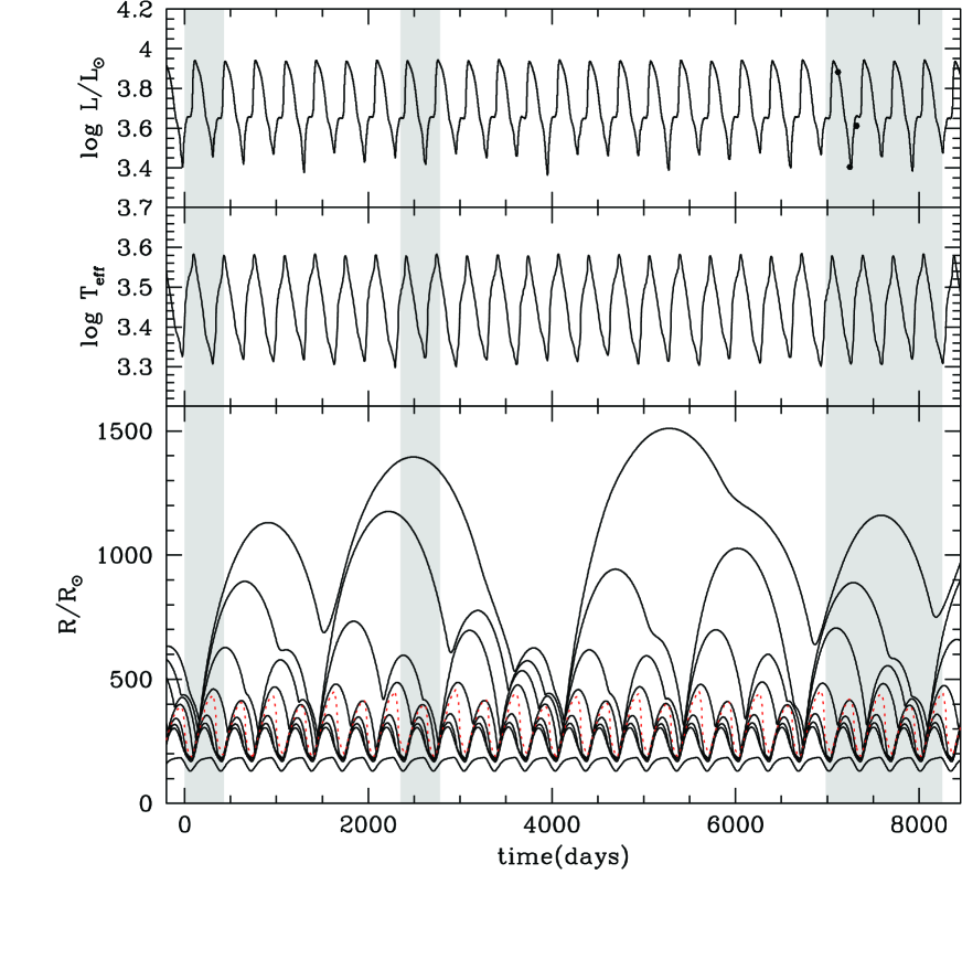
Figure 1: The luminosity (top panel), effective temperature (center panel) and radius of selected mass zones (lower panel) as a function of time for the o54 pulsation model. The red dashed line in the bottom panel corresponds to the radius at Rosseland mean optical depth 2/3, and the effective temperature ($\propto(L/R^{2})^{0.25}$) refers to this radius.

2.2 The atmospheric models

With the gas pressure fixed from the dynamical models, the gas and dust temperatures in the photosphere are re-solved by using an opacity-sampling method in LTE. This is in contrast to previous models of Mira atmospheres that used a small 72-wavelength averaged-opacity mesh (e.g. Hofmann et al., 1998; Ireland et al., 2004b, a; Ireland & Scholz, 2006) or 51-wavelength mesh (e.g. Höfner et al., 2003). Our continuum and Just-Overlapping-Line-Approximation (JOLA) VO opacities are the same as in Hofmann et al. (1998). The continuum opacity sources (free-free and bound-free where applicable) are H, H-, H₂, H₂-, He- and Thompson scattering. The H₂O lines come from Partridge & Schwenke (1997) and those of TiO from Schwenke (1998). Other diatomic molecular (CO, OH, CN, SiO, MgH) and neutral atomic lines (Na, Mg, Al, K, Ca, Ti, V, Cr, Mn, Fe,and Ni) come from the input to the ATLAS12 models (Kurucz, 1994). The lack of metal bound-free opacities means that our models are inaccurate at wavelengths shortwards of 450 nm: wavelengths that are both unimportant energetically in the atmospheric layers modelled by the opacity-sampling code and strongly affected by numerous other approximations such as LTE.

A micro-turbulence of 2.8 km/s is assumed, in between that used in the M-giant models of Plez et al. (1992) and that derived by Hinkle & Barnes (1979). Line profiles for molecules are taken to be Gaussian, as pressure-broadening is negligible and the opacity is dominated by a very large number of weak lines. For atomic lines, a Voigt profile is assumed, with only radiative damping taken into account with a nominal $\Gamma$ value of $10^{8}$, typical of atomic transitions. The equation of state is based on that used in Tsuji (1973), with 35 atoms and their first 2 positive ionization states, 60 molecules, H-, H₂- and F-. The chemical equilibrium constants for CO, MgH, SiH and TiO₂ have since been measured more accurately and differ significantly from Tsuji (1973), so for these molecules we have adopted constants from Sharp & Huebner (1990). We assume solar abundances, and take the solar abundances from Grevesse et al. (1996).

The dust opacity and equation of state is taken from the approximations of Ireland & Scholz (2006), with parameters designed to best fit dust scattering opacity observations: the log of the number of nuclei per H atom $\log(N_{\rm nuc})=-12.8$ and the ratio of sticking coefficients $\alpha_{s}=1$. This treatment of dust opacity is temperature-dependent, due to the $\sim 1\mu$m dust opacity being a strong function of the Fe-content of the dust, only approaching standard interstellar medium dust opacities (e.g. Draine & Lee, 1984) at $T\la 1000K$.

The opacities are calculated for 4300 wavelengths running from 200 nm to 50 $\mu$m, with 1 nm sampling between 200 nm and 3 $\mu$m and sampling proportional to $\lambda^{3}$ for longer wavelengths. The effect of the velocity stratification on the radiative transfer is not taken into account, but is expected to have significant effects only in the vicinity of shock fronts (see Section 3).

Instantaneous relaxation of shock heating behind the moving shock front is assumed (see discussion in Bessell et al., 1989). This is equivalent to enforcing $L=L_{\rm surf}$ everywhere, with $L_{\rm surf}$ the model surface luminosity. Although the shock luminosity is important for modelling emission lines, its luminosity is generally negligible in the photospheric regions where the continuum is optically thin and where lines are formed. At phases immediately before maximum luminosity, as the light curve of a Mira is rapidly rising, the shock luminosity can for a small time reach half the model luminosity. The assumption $L=L_{\rm surf}$ is incorrect in this case, meaning that the shape of the continuum during this rapid pre-maximum flux increase phase may not be a good approximation. The effects of this approximation are examined further in Section 3.3.

The equation of radiative transfer is solved using the same code as Schmid-Burgk & Scholz (1984), with up to 80 discrete depth points. Since this code uses a spline interpolation, the pressure discontinuity at the shock front is smoothed out over 0.05$R_{p}$ (deep layers) to 0.1$R_{p}$ (high layers). The model outer-boundary is fixed at 5 $R_{p}$: a boundary where the dust formation is more complex than our simple approximations allow, and where radiative acceleration on dust can influence the dynamics significantly. Layers outside 5 $R_{p}$ can be considered the ‘wind’ zone, and can be seen observationally only in the mid-infrared due to dust opacity and in the strongest of molecular transitions.

Once the equation of radiative transfer is solved, the spectrum and center-to-limb profile is computed over a finer wavelength grid, typically with 17000 wavelengths. This finer grid includes wavelength in the radio regime, where the wavelength-dependence of free-free opacities means that the continuum photospheric radius is quite different to that in the near-infrared Reid & Menten (2007).

3 Discussion of model quality

3.1 Verification of opacity-sampling code for a static model

Previously published models for static extended M-giant atmospheres from other groups (Fluks et al., 1994; Hauschildt et al., 1999) have demonstrated relatively good agreement with observations. Therefore, as a first step in verifying the performance of our code, we will compare the model spectra for a relatively compact static model to those from the PHOENIX code. This code has also adopted LTE for published models (Hauschildt et al., 1999), so if the input opacities to their models and our models were the same, one would expect the model outputs to be the same. As a comparison model, we choose a 5 solar-mass model with log($g$)=0 (cgs units), and $T_{\rm eff}=3200$ K. This model is one of the most extended configurations from Hauschildt et al. (1999), which is not designed for very extended atmospheres, and is the most compact model where our numerical approximations still solve the equation of radiation transport with reasonable accuracy.

Figure 2 shows the model spectra comparison between 1 and 3.0 $\mu$m, and Figure 3 shows the comparison between 0.5 and 1 $\mu$m. The most noticeable difference is the depth of the TiO features: the dominant molecular bands short-wards of 1 $\mu$m. Some of this difference comes from the use of the Jørgensen (1994) line list by Hauschildt et al. (1999) (N.B. more recent PHOENIX models of M-dwarfs use the same TiO opacity as we do). When the Jørgensen (1994) line list is used with the CODEX models (adopting the oscillator strengths from Allard et al., 2000), the difference at around 750 nm becomes smaller and the details of the band shapes agree more, as seen in Figure 3. The discrepancy in the TiO feature at 1.25 $\mu$m as shown in Figure 2 is also reduced using this line list (not shown). However, the overall flux level of models the at shorter wavelengths, particularly between 500 and 700 nm remains discrepant. Both reducing the effective temperature of our models by $\sim$100 K and using the Jørgensen (1994) line list produces a very small difference between the CODEX and PHOENIX models (not shown).

We also compare the 3200 K static model to observations in Figure 5, where an M6 and an M7 spectrum is compared to the models. We note that the difficulties in our models fitting the gap between the strong TiO bands at 750 nm is in common with the current version of the PHOENIX models (e.g. see Lançon et al., 2007), due to an inadequacy in the line lists. Until this line list is updated, spectral indices based on TiO absorption will not be able to be used to convert the model spectra to spectral types.

At $\sim 2.5\mu$m, the PHOENIX models have a feature that is not in our models: presumably this is due to the difference in water line lists: again the line list used by us is that adopted in more modern PHOENIX dwarf models and not the published PHOENIX giant models. There is also a difference in the temperature structure of the models, as seen in Figure 4. We have independently checked the temperature structure of our models using a (computationally slow) Interactive Data Language (IDL) radiative transfer code that uses the a modified Unsöld-Lucy temperature correction for spherical atmospheres (e.g. Hauschildt et al., 1999) and trapezoidal-rule integration, finding differences of order 10 K only, so we therefore expect the difference in temperature structure to be due to further opacity differences rather than computational errors.

Note that previous versions of our code, such as that used in Ireland et al. (2004b, a) could not reproduce the spectra of these static models nearly so well, due to the inaccuracies of the Just Overlapping Line Approximation at these low to moderate TiO optical depths (e.g. Brett, 1990; Tej et al., 2003).

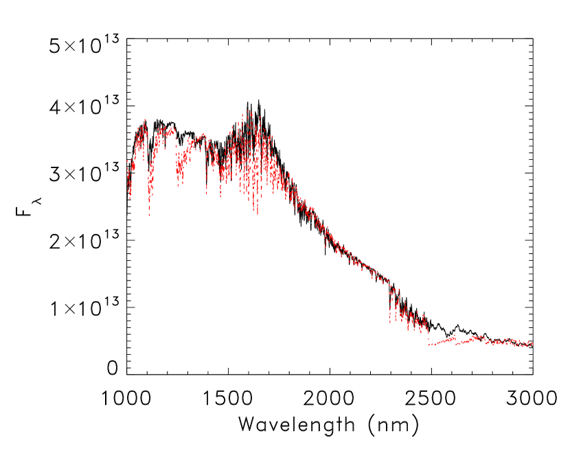
Figure 2: The spectrum between 1 and 3.0 $\mu$m produced from the CODEX atmosphere models at 3200 K (solid lines), compared with that from the PHOENIX atmosphere code (red dotted line).

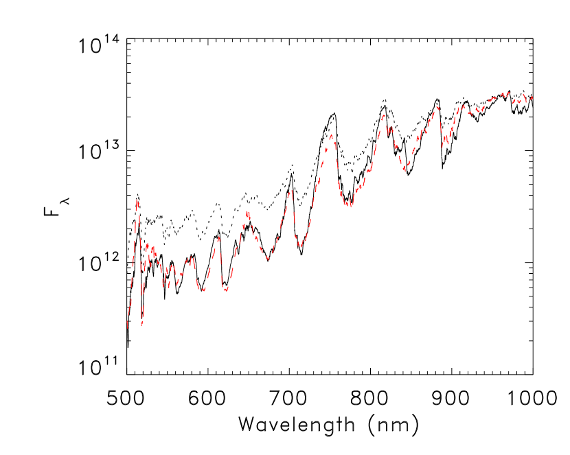
Figure 3: The spectrum between 0.5 and 1.0 $\mu$m produced from the CODEX atmosphere models at 3200 K (solid lines), compared with that from the PHOENIX atmosphere code (dotted line), and the CODEX models using the same TiO line list as PHOENIX (red dashed line) (see text).

Figure 4: The temperature profile of the CODEX models for a 3200 K model (solid line) plotted with the the PHOENIX models (dashed line) for the same model parameters.

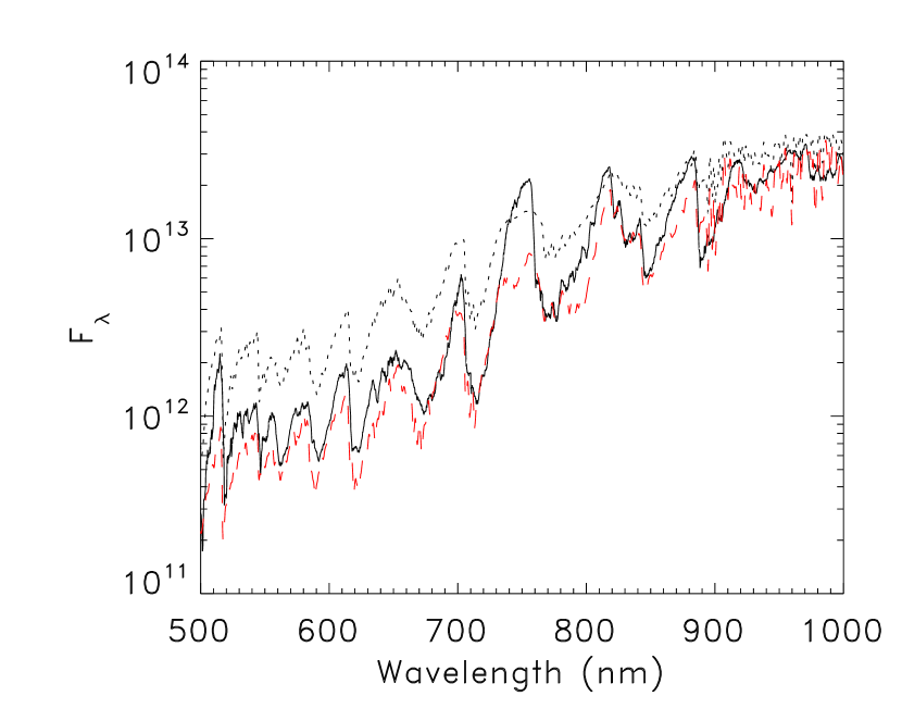
Figure 5: The spectrum between 0.5 and 1.0 $\mu$m produced from the CODEX atmosphere models at 3200 K (solid lines), compared with an M6 giant spectrum (upper dotted line) and M7 giant spectrum (lower red dashed line) from Fluks et al. (1994).

3.2 Critical assumptions examined at 3 model phases

There are a large number of computational checks one can make on the quality of our atmospheric models before comparing them directly to observations. The checks that we consider most relevant will be presented here, relating directly to model physical assumptions and approximations: 1) Is a grey temperature-profile adequate for describing the atmospheric dynamics?; 2) Does the velocity stratification significantly influence the solution to the radiative transfer equation?; 3) How much does the LTE approximation affect the spectrum and temperature profile?; and 4) How does neglecting the shock luminosity by insisting “$L=L_{\rm surf}$” everywhere affect the model properties? We will attempt to answer these questions by examining three model phases in detail. The 3 models have phases of 0.20 0.59 and 0.80 relative to (estimated) maximum bolometric luminosity, which is assigned phase 0.0.

Using a grey model for the non-linear dynamical models is only valid to the extent that the temperature profile is consistent with that from a more accurate non-grey model. Furthermore, the grey model uses approximations for the spherically-extended atmosphere that also affect the way that radiative acceleration is calculated. Figure 6 shows the grey and non-grey temperature profiles, and the grey and non-grey accelerations as a function of radius. The total acceleration includes a gravitational term, a gas pressure term and a radiative acceleration term:

$$a=g+\frac{1}{\rho}\frac{dP_{\rm gas}}{dr}+\frac{\pi}{c}\int_{0}^{\infty}k_{\nu}F_{\nu}d\nu.$$ (1)

Here $k_{\nu}$ is the extinction coefficient at frequency $\nu$, $F_{\nu}$ is the monochromatic flux per unit frequency and other terms have standard meanings.

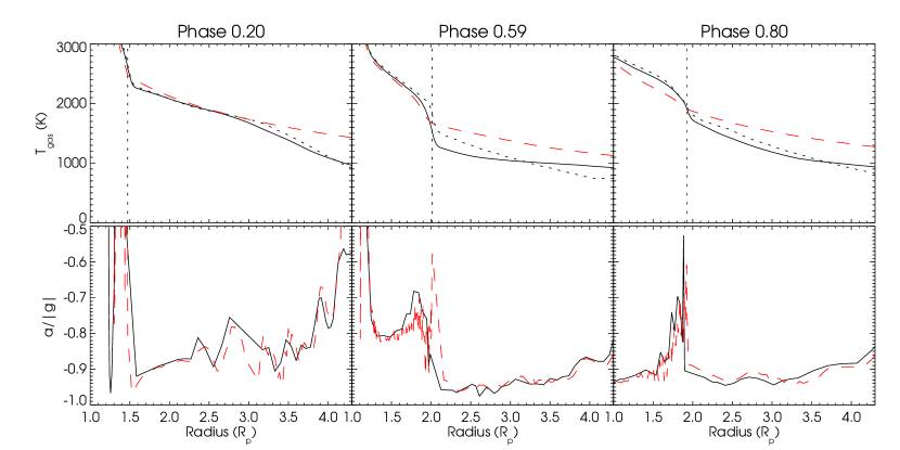
Figure 6: A comparison between the grey dynamical model temperature profile and total acceleration as a fraction of gravity (red dashed-lines) with that from the non-grey opacity-sampling code (solid lines), for the fx series models at phases 0.20 (left), 0.59 (center) and 0.80 (right) from the same cycle. The ‘spikes’ in the acceleration are near the location of shock fronts and are an artifact of smoothing the shock front in the dynamical grey and non-grey models. The dominant shock fronts are marked with vertical dotted lines, and the dotted lines in the top panel are temperatures calculated with the 72 mesh wavelength grid as in Ireland et al. (2004b).

This figure demonstrates first that the grey approximation only affects temperatures in the outer layers at the 10-20% level (excluding shock fronts). A 10% increase in the grey model temperature would cause a 10% increase in the pressure gradient for the same mass stratification. This in turn changes the acceleration (both continuous acceleration and the $\delta$-function acceleration at a shock-front) at the 10% level. During a pulsation cycle, the bulk of the non-gravitational acceleration of a given layer occurs close to the continuum-forming photosphere, where the diffusion approximation as used in the grey model is most accurate. The gas in the outer layers follows near-ballistic trajectories. Therefore, we estimate that geometric pulsation amplitudes for layers between 1 and 4 $R_{p}$ are accurate to $\la$10%.

As a dynamic atmosphere has a velocity stratification $v(r)$, the radiation field seen from a test point at a spectral-line wavelength may strongly depend, as a consequence of Doppler shifting, on the depth of the layer of origin and on the direction of the line-of-sight. There are two classes of $v(r)$ effects: a geometric $v(r)$ projection effect that is often moderate except for the very most extended atmospheres; and more significant effects at and near a shock front where $v(r)$ is discontinuous at and has a strong gradient near the position of the shock. Sample wavelengths that, e.g., are located at line frequencies within a forest of blanketing lines below the shock appear in the continuum above the shock, and vice versa. This may lead to substantial errors in computed equilibrium temperature when an opacity sampling technique is used for treating radiative transport that is dominated by line blanketing. Solutions for the case of a velocity stratification $v(r)$ have been developed for the opacity distribution technique, though for only rather simple cases of $v(r)$ (e.g. Baschek et al., 2001; Wehrse et al., 2003; Castor, 2004), but no solutions are known for the opacity sampling method (which necessarily has large gaps in-between individual wavelengths that are sampled).

We have, however, numerically examined the equation of radiative transfer in the dynamical model atmosphere without attempting a full solution. This was accomplished by calculating the luminosity at each layer of a model stratification on a grid of $\sim 10^{6}$ wavelengths, self-consistently taking into account the velocity of each layer, by red-shifting or blue-shifting the line profiles according to the difference in projected velocities. This code was far too slow to attempt a solution to the equation of radiative transfer, but could examine the departure from the $L=L_{\rm surf}$ criterion. Figure 7 shows a maximum 2 % deviation from the $L=L_{\rm surf}$ criterion, demonstrating that the effects of the dynamical stratification are a relatively minor effect in calculating the temperature structure. The effects of the dynamical structure on the overall spectral shape was also examined and also found to be minor, as shown in Figure 8.

Deviations from LTE tend to increase with decreasing densities and pressures. With typically very low pressures ($<1$ dyn cm^-2) in the atmospheric regions of Mira variable stars where spectral features are formed, these stars are a long way from LTE. This is because collisions can not thermalise the level populations of atoms and molecules. Non-LTE effects are most noticeable for electronic transitions of atoms and TiO, where typical Einstein A coefficients of $\sim 10^{7}$s^-1 greatly exceed collisional rates of order $10^{2}$ s^-1. Note that this is quite different to the CO molecule, where Einstein A coefficients for vibrational transitions are of order $10^{1}$ s^-1 (Chandra et al., 1996).

These non-LTE effects for TiO are much more important in Miras than in static M giants, despite static M giants also having Einstein A coefficients much higher than collisional rates. This is because static M giant atmospheres are not nearly as extended as Miras, so the thin outer layers are much warmer for the same continuum-forming temperature. In turn, this means that the band depths calculated in LTE are much deeper for Miras, increasing the potential for non-LTE effects to be important in modelling.

A complete band-model non-LTE treatment of TiO opacity would require a complete new radiative transfer code (both codes used in this paper tabulate opacities as a function of LTE temperature and pressure). However, we have attempted to treat the TiO absorption with a partial band-model non-LTE treatment in order to examine some effects of the LTE approximation.

We make an assumption that the electronic singlet and triplet ground states for TiO are populated in thermal equilibrium (i.e. in both rotational and vibrational equilibrium), and that transitions to and from excited electronic states occur via scattering processes. Both resonance and fluorescence scattering processes are included. This assumption is reasonable because radiative transitions between vibrational levels are dominated by direct ro-vibrational transitions for radiation field temperatures of $\sim$1500 K (applicable to the region where the strong TiO features form). These ro-vibrational transitions see a thermalised radiation field due to strong mid-infrared transitions of other molecules (notably H₂O). Radiative transitions between electronic excited states (multi-photon absorption) is not as important here as it is for many atomic states because of the relatively large gap between the ground and first electronic excited state (i.e. in layers where the strong features are formed, the molecule spends the vast majority of its time in the electronic ground state). Collisions with other atoms and molecules are also negligible in the regions where the strongest features are formed.

Figure 7: A comparison between the luminosity as a function of radius between the opacity-sampling code (straight dashed lines) and full dynamical modelling taking into account all wavelengths and the velocity stratification (solid lines). The models, from top to bottom, are at phases 0.20 (7623 L_⊙), 0.80 (4092 L_⊙), and 0.59 (2548 L_⊙).

The scattering process is added to the equation for the source function as follows:

$$S(\lambda)=\frac{\kappa(\lambda)B(\lambda)+\int\sigma(\lambda,\lambda^{\prime})J(\lambda^{\prime})d\lambda^{\prime}}{\kappa(\lambda)+\int\sigma(\lambda^{\prime},\lambda)d\lambda^{\prime}}.$$ (2)

$S$, $B$, $J$ and $\kappa$ have their usual meanings of source function, Planck function, mean intensity and absorption coefficient (cross-section per unit mass). The isotropic scattering matrix $\sigma(\lambda,\lambda^{\prime})$ describes scattering from wavelength $\lambda^{\prime}$ to wavelength $\lambda$, in units of cm²/g/nm. For resonant (i.e. non-fluorescent) scattering, $\sigma(\lambda^{\prime},\lambda)=\delta(\lambda-\lambda^{\prime})\sigma(\lambda)$, with $\delta$ the Dirac $\delta$-function.

The results of this calculation is shown in Figure 8. It is clear that fluorescence scattering in general dominates the radiative processes in the $V$-band, and that interpretations such as the simplified LTE interpretation of Reid & Menten (1997) offer a gross over-simplification of the physical processes that create the visible light-curves of Mira variables. This statement is true both in the strong absorption bands and in the regions of weaker absorption in-between the bands. Note that a similar fluorescence approach would have to be applied to VO in order to model the 0.75 to 1.2 micron region more accurately.

The models still do not well-represent the deep TiO features, as will be discussed in Section 4. A possible explanation for this discrepancy is inaccurate data for TiO₂, that could enable TiO to be removed from the gas at higher temperatures (e.g. Ireland et al., 2005; Ireland & Scholz, 2006), or non-equilibrium processes in the chemical reactions of TiO. An example of such a non-equilibrium process is the lowering of the vibrational temperature of TiO as the mid-infrared regions of the spectrum become optically-thin and the justification for the fluorescence scattering approximation above no longer work. This would drive the reaction TiO+H₂O$\rightleftharpoons$TiO₂+H₂ to the right, removing TiO from the gas. This kind of complexity is beyond the capabilities of the code developed for this paper.

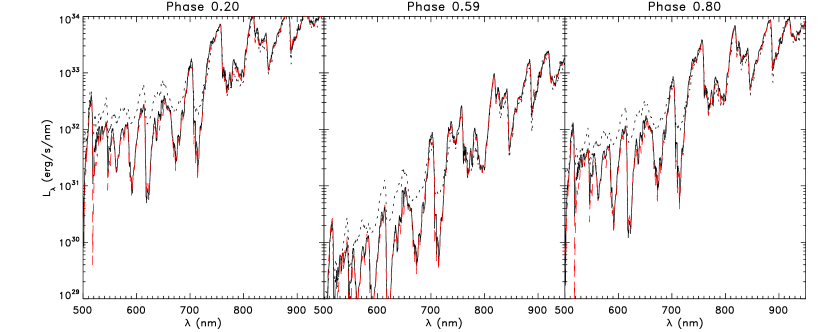
Figure 8: A comparison between the opacity-sampling code spectrum (solid lines) between 500 and 950 nm and that resulting from a fluorescence scattering non-LTE treatment of the opacity (dotted lines). The dynamical atmosphere calculation is also shown (red dashed lines), demonstrating that this effect is very small compared with non-LTE effects.

3.3 Other model quality issues

The opacity-sampling method for radiative transfer calculations is only valid if a large enough number of wavelengths are used. For several representative test models with different stellar parameters (in particular different effective temperature), we have solved the radiative transfer equation based on the here adopted 4300-wavelength mesh, as well as meshes with 2152 and 8606 wavelength samples. Differences of temperatures never exceeded a few tens of degrees in high layers for the 4300 vs. 2152 case, and were negligible for the 4300 vs. 8606 case. Typically, including dust absorption that makes the atmospheric high-layer opacity ”greyer”, diminishes 4300 vs. 2152 differences. We also increased strongly heavy-element abundances, i.e. the effects of line blanketing upon the temperature stratification, and found increasing and significant 4300 vs. 2152 differences whereas no 4300 vs. 8606 differences showed up. Thus, a 4300-wavelength mesh is well suited to cover even quite unfavorable cases of M-type Mira atmospheres. Temperature errors of the order of a few tens of degrees are smaller than other errors such as those caused by the smoothing of shock fronts, the dynamic stratification, or non-LTE effects. We note that the opacity-sampling models of Höfner & Andersen (2007) with only 64 wavelength points are not expected to have sufficient wavelength sampling to accurately reproduce the temperature-profile. However, those models also used a 64-wavelength opacity-sampling method for the dynamic atmosphere computation, which may be preferable to our grey dynamical models.

As seen in Figure 6, the temperature profiles of the CODEX models differ noticeably from the profiles computed from the models of Ireland et al. (2004b), where the opacities were mainly approximated by mean opacities over 72 wavelength bins and dust formation was not included. We see the current models as a major improvement over those models. This older style of opacity computation was intermediate between the current opacity sampling method and a grey atmosphere, as can be seen from the temperature profile over the range 1000 to 2000 K. At the lowest temperatures ($\la 1000$ K), the CODEX models are warmed more than these older models because of the presence of dust.

In addition to limitations evident from the tests above, the CODEX models have clear limits where unknown details of complex heterogeneous dust formation become important, and could not be used to model e.g. OH/IR stars. These approximations are discussed in detail in Ireland & Scholz (2006). Importantly, dust is assumed to form in equilibrium, which is only applicable to the hottest ($\ga$1000 K) dust.

Finally, we have performed test calculations where the $L=L_{\rm surf}$ approximation is removed, and the shock luminosity is added to the models over a smoothed region of size $\Delta r/r\sim 5$%. The only test model with a noticeable (i.e. above numerical errors) change in model structure was the phase 0.80 model, which had a 540 $L_{\odot}$ shock within the continuum-forming photosphere and a total luminosity of 4090 $L_{\odot}$. The model that included the shock luminosity had 5% less H-band flux and 10% more V-band flux. As this phase is at the time where the model luminosity (and light curve of observed Miras) is rapidly increasing prior to maximum luminosity, these differences are not very significant.

4 Reliable Observational Predictions

Given that Section 3 demonstrated that there are some approximations that are not physically realistic, we will examine which model outputs are most reliable for comparison to observations. Clearly, only those regions of the spectrum that are well-approximated by LTE should give reasonable agreement to observations. The phase, cycle and parameter dependence of predictions will be examined in a forthcoming paper II.

4.1 Spectra

Figure 9 shows some observed spectra compared with models. Instead of spectra of $o$ Ceti, that were not readily available in electronic form, we chose to compare the models with R Cha, a Mira with a 335 day period: almost exactly the same as $o$ Ceti. For phases 0.2 and 0.59, an observed spectrum is available at a close enough model phase to give reasonable spectral agreement between the CODEX models and observations. In particular, the near-minimum spectrum is much better represented by the CODEX model than by the previous generation of models as examined in Tej et al. (2003). The infrared features of H₂O and CO are reproduced reasonably, but the TiO features remain too deep in the CODEX models. Although some of this discrepancy is explained by the effect of the LTE approximation, the test calculation results shown in Figure 8 demonstrate that a fluorescence scattering approximation does not noticeably affect band depths long-wards of 750 nm. Therefore, we can not consider the band depths of strong TiO features to be a reliable prediction, with or without the addition of fluorescence scattering. The infrared features, particularly those short-wards of 2500 nm, are expected to be a reasonably good model prediction.

The visible-light spectrum and flux is too small to be seen on the linear scale in Figure 9. As visible light curves are one of the richest data sets for Mira variables, theoretical predictions for these curves as a function of physical parameters is a major goal of our effort. As visible wavelengths are in the Wien part of the Planck function at temperatures relevant to Miras, fluxes and spectra are very sensitive to changes in the atmospheric stratification. The effects of the LTE approximation as discussed in Section 3.2 cause visible fluxes to be underestimated by a factor of $\sim$2. The difficulty in accurately treating dust can give another few tens of % error. So we expect the model-predicted visible light curve to have uncertainties of approximately 1 magnitude.

4.2 Diameters

In Figure 10, we show the range of model-predicted diameters for $o$ Ceti for the three phases examined. In order to make this plot, we calculated visibility curves for filters with 1% fractional bandwidth and calculated the best fit uniform-disk visibility curves at $V=0.6$ and $V=0.2$. The fitted angular diameter can be a strong function of where this fit is made (e.g Ireland et al., 2004b). We assume a distance of 100 pc after van Leeuwen (2007) for this plot. We also show measured diameters from Ireland et al. (2004c) ($<1$ $\mu$m) and Woodruff et al. (2008) (1-4 $\mu$m). We do not show mid-infrared diameters from Weiner et al. (2003), because of the complexity of accounting for the over-resolved dust emission from the wind. The error bars represent both observational error and the differences amongst observations at different phases. The J-band diameter range of the models match the observations very well, showing that the continuum diameters are in good agreement: certainly within 10% in diameter, corresponding to 5% in effective temperature. However, the measured diameters at H, K and L bands are always close to the largest model diameters. We suspect this not to be an error in modelling, but instead a physical effect demonstrating that $o$ Ceti is usually surrounded by more extended molecular layers than the present models produce. Changing e.g. the assumed model mass may help resolve this small discrepancy.

In Ireland & Scholz (2006), we showed that the diameters of Mira variables at wavelengths shorter than 1 $\mu$m were in general well-described by the model of dust formation that we use here, consistent with Figure 10. However, this statement was not true for the strong TiO absorption bands, in particular the band at 712 nm. The inclusion of the fluorescence scattering approximation as a test calculation in this paper greatly increases the model diameters in the TiO absorption bands (as seen by the dotted line), meaning that, where necessary, more accurate predictions for model diameters short-wards of 1 $\mu$m can now be produced.

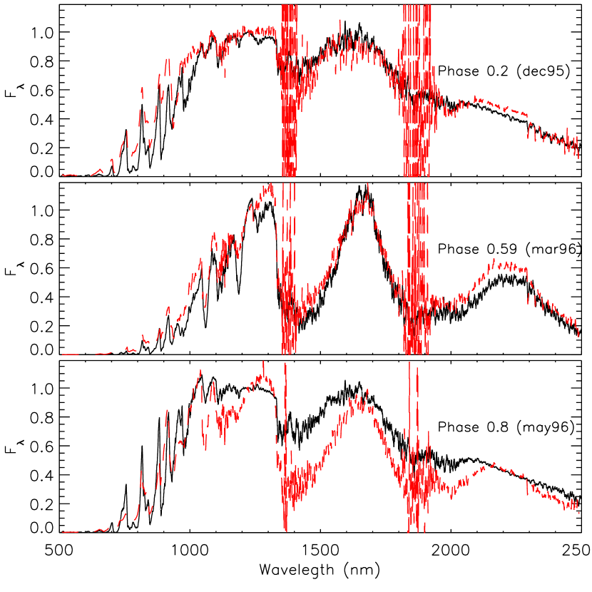
Figure 9: Smoothed model spectra (black solid lines), with measured spectra of R Cha from Lançon & Wood (2000) over-plotted (red dashed lines). The plots are labeled by their model phases. The estimated visual phases of the observations are 0.25, 0.5 and 0.76.

Figure 10: Model diameters between 0.6 and 4 $\mu$m for the CODEX models (dashed lines) and the models with the fluorescence scattering approximation for TiO (dotted line). The range shown corresponds to the maximum and minimum diameters of the three models using two fitting techniques (see text). The horizontal axis is linear in wave-number so that both the full range and the TiO features can be shown. Points with error bars show the range of measured diameters from Ireland et al. (2004c) and Woodruff et al. (2008).

5 Conclusions and Future Work

We have presented the Cool Opacity-sampling Dynamic EXtended (CODEX) modelling method: an improved scheme for constructing stellar atmosphere models that is tailored to Mira variable star atmospheres. This scheme includes self-excited pulsation and a 4300-wavelength grid opacity-sampling code to solve for the equation of radiative transfer.

The models stand up to a variety of numerical tests, including adequate treatment of shock fronts and dynamical effects, and sensitivity at less than the 10% to the grey approximation used in the dynamical models. The models notably have a $\sim$100 K maximum difference in temperature profile when benchmarked against static PHOENIX models, which give the CODEX models deeper absorption shortwards of 950 nm. Test calculations using a fluorescence scattering approximation for non-LTE TiO effects demonstrated a modest difference in overall energetics, but a factor of $\sim$2 increase in V-band flux and much larger diameters in TiO absorption bands.

Model predictions from the series presented here, as well as future work, will be be made available online. Work in progress includes the detailed analysis of the phase and cycle dependence of model properties, models with different fundamental parameters including stars with longer periods and modified element abundances (metallicity, S-type C/O ratio, modified N abundance), as well as further comparison of typical model predictions with observed features.

References

- Allard et al. (2000) Allard F., Hauschildt P. H., Schwenke D., 2000, ApJ, 540, 1005
- Baschek et al. (2001) Baschek B., Waldenfels W. V., Wehrse R., 2001, A&A, 371, 1084
- Bessell et al. (1989) Bessell M. S., Brett J. M., Scholz M., Wood P. R., 1989, A&A, 213, 209
- Bowen (1988) Bowen G. H., 1988, ApJ, 329, 299
- Bressan et al. (1993) Bressan A., Fagotto F., Bertelli G., Chiosi C., 1993, A&AS, 100, 647
- Brett (1990) Brett J. M., 1990, A&A, 231, 440
- Castor (2004) Castor J. I., 2004, Radiation Hydrodynamics. Radiation Hydrodynamics, by John I. Castor, pp. 368. ISBN 0521833094. Cambridge, UK: Cambridge University Press, November 2004.
- Chandra et al. (1996) Chandra S., Maheshwari V. U., Sharma A. K., 1996, A&AS, 117, 557
- Draine & Lee (1984) Draine B. T., Lee H. M., 1984, ApJ, 285, 89
- Feast et al. (1989) Feast M. W., Glass I. S., Whitelock P. A., Catchpole R. M., 1989, MNRAS, 241, 375
- Ferguson et al. (2005) Ferguson J. W., Alexander D. R., Allard F., Barman T., Bodnarik J. G., Hauschildt P. H., Heffner-Wong A., Tamanai A., 2005, ApJ, 623, 585
- Fluks et al. (1994) Fluks M. A., Plez B., The P. S., de Winter D., Westerlund B. E., Steenman H. C., 1994, A&AS, 105, 311
- Fox & Wood (1982) Fox M. W., Wood P. R., 1982, ApJ, 259, 198
- Grevesse et al. (1996) Grevesse N., Noels A., Sauval A. J., 1996, in ASP Conf. Ser. 99: Cosmic Abundances, Holt S. S., Sonneborn G., eds., p. 117
- Hauschildt et al. (1999) Hauschildt P. H., Allard F., Ferguson J., Baron E., Alexander D. R., 1999, ApJ, 525, 871
- Hinkle & Barnes (1979) Hinkle K. H., Barnes T. G., 1979, ApJ, 227, 923
- Hofmann et al. (1998) Hofmann K.-H., Scholz M., Wood P. R., 1998, A&A, 339, 846
- Höfner & Andersen (2007) Höfner S., Andersen A. C., 2007, A&A, 465, L39
- Höfner et al. (2003) Höfner S., Gautschy-Loidl R., Aringer B., Jørgensen U. G., 2003, A&A, 399, 589
- Höfner et al. (1998) Höfner S., Jørgensen U. G., Loidl R., Aringer B., 1998, A&A, 340, 497
- Hughes & Wood (1990) Hughes S. M. G., Wood P. R., 1990, AJ, 99, 784
- Ireland & Scholz (2006) Ireland M. J., Scholz M., 2006, MNRAS, 367, 1585
- Ireland et al. (2004a) Ireland M. J., Scholz M., Tuthill P. G., Wood P. R., 2004a, MNRAS, 355, 444
- Ireland et al. (2004b) Ireland M. J., Scholz M., Wood P. R., 2004b, MNRAS, 352, 318
- Ireland et al. (2004c) Ireland M. J., Tuthill P. G., Bedding T. R., Robertson J. G., Jacob A. P., 2004c, MNRAS, 350, 365
- Ireland et al. (2005) Ireland M. J., Tuthill P. G., Davis J., Tango W., 2005, MNRAS, 361, 337
- Jeong et al. (2003) Jeong K. S., Winters J. M., Le Bertre T., Sedlmayr E., 2003, A&A, 407, 191
- Jørgensen (1994) Jørgensen U. G., 1994, A&A, 284, 179
- Jura & Kleinmann (1992) Jura M., Kleinmann S. G., 1992, ApJS, 79, 105
- Keller & Wood (2006) Keller S. C., Wood P. R., 2006, ApJ, 642, 834
- Knapp et al. (2003) Knapp G. R., Pourbaix D., Platais I., Jorissen A., 2003, A&A, 403, 993
- Kurucz (1994) Kurucz R. L., 1994, in LNP Vol. 428: IAU Colloq. 146: Molecules in the Stellar Environment, Jørgensen U.G. ed., Vol. 428, p. 282
- Lançon et al. (2007) Lançon A., Hauschildt P. H., Ladjal D., Mouhcine M., 2007, A&A, 468, 205
- Lançon & Wood (2000) Lançon A., Wood P. R., 2000, A&AS, 146, 217
- Marconi & Clementini (2005) Marconi M., Clementini G., 2005, AJ, 129, 2257
- Partridge & Schwenke (1997) Partridge H., Schwenke D. W., 1997, J. Chem. Phys., 106, 4618
- Plez et al. (1992) Plez B., Brett J. M., Nordlund A., 1992, A&A, 256, 551
- Reid & Menten (1997) Reid M. J., Menten K. M., 1997, ApJ, 476, 327
- Reid & Menten (2007) Reid M. J., Menten K. M., 2007, ApJ, 671, 2068
- Rogers & Iglesias (1992) Rogers F. J., Iglesias C. A., 1992, ApJ, 401, 361
- Schmid-Burgk & Scholz (1984) Schmid-Burgk J., Scholz M., 1984, Transfer in spherical media using integral equations, Methods in Radiative Transfer, Kalkofen W. Ed., pp. 381–394, Cambridge Univ. Pr., Cambridge UK
- Schwenke (1998) Schwenke D. W., 1998, in Chemistry and Physics of Molecules and Grains in Space. Faraday Discussions No. 109, p. 321
- Sharp & Huebner (1990) Sharp C. M., Huebner W. F., 1990, ApJS, 72, 417
- Tej et al. (2003) Tej A., Lançon A., Scholz M., Wood P. R., 2003, A&A, 412, 481
- Tsuji (1973) Tsuji T., 1973, A&A, 23, 411
- van Leeuwen (2007) van Leeuwen F., 2007, Hipparcos, the New Reduction of the Raw Data. Hipparcos, the New Reduction of the Raw Data, Astrophysics and Space Science Library, Vol. 350 20 Springer Dordrecht
- Wehrse et al. (2003) Wehrse R., Baschek B., von Waldenfels W., 2003, A&A, 401, 43
- Weiner et al. (2003) Weiner J., Hale D. D. S., Townes C. H., 2003, ApJ, 588, 1064
- Whitelock et al. (2000) Whitelock P., Marang F., Feast M., 2000, MNRAS, 319, 728
- Woitke (2006) Woitke P., 2006, A&A, 452, 537
- Wood (1979) Wood P. R., 1979, ApJ, 227, 220
- Wood & Zarro (1981) Wood P. R., Zarro D. M., 1981, ApJ, 247, 247
- Woodruff et al. (2008) Woodruff H. C., Tuthill P. G., Monnier J. D., Ireland M. J., Bedding T. R., Lacour S., Danchi W. C., Scholz M., 2008, ApJ, 673, 418