Phase Closure Image Reconstruction for Future VLTI Instrumentation

Abstract

Classically, optical and near-infrared interferometry have relied on closure phase techniques to produce images. Such techniques allow us to achieve modest dynamic ranges.

In order to test the feasibility of next generation optical interferometers in the context of the VLTI-spectro-imager (VSI), we have embarked on a study of image reconstruction and analysis. Our main aim was to test the influence of the number of telescopes, observing nights and distribution of the visibility points on the quality of the reconstructed images. Our results show that observations using six Auxiliary Telescopes (ATs) during one complete night yield the best results in general and is critical in most science cases; the number of telescopes is the determining factor in the image reconstruction outcome.

In terms of imaging capabilities, an optical, six telescope VLTI-type configuration and $\sim$200 meter baseline will achieve 4 mas spatial resolution, which is comparable to ALMA and almost 50 times better than JWST will achieve at 2.2 microns. Our results show that such an instrument will be capable of imaging, with unprecedented detail, a plethora of sources, ranging from complex stellar surfaces to microlensing events.

1 INTRODUCTION

Image reconstruction is a key problem in observational astronomy, in particular in optical interferometry, where it is needed to overcome existing ambiguities in the interpretation of simple visibility measurements.

In an array of N telescopes, signals are combined in $\frac{1}{2}$ $\times$ N $\times$ (N-1) pairs or baselines to obtain $\frac{1}{2}$ $\times$ N $\times$ (N-1) measurements called complex visibilities. These visibilities are related to the object brightness distribution via the van Cittert-Zernike theorem:

$V(u,v)=\int\int I(x,y)\,exp[-2\,\pi\,i\,(ux+vy)]dx\,dy$

where x and y are angular displacements on the plane of the sky with the phase center as origin, I(x,y) is the brightness distribution of the target and u and v are the position vectors of the baselines projected on a plane perpendicular to the source direction, which together define the uv plane. In practical terms, the better the sampling of the uv plane in terms of baseline length, position angle, and number of measurements, the more faithful the reconstructed image will be relative to the true brightness distribution.

In order to recover the brightness distribution, several image reconstruction algorithms for interferometry have been developed: phase referencing using aips, hybrid mapping using difmap (Masoni et al. 2005, Masoni 2006), the building block bispectrum method (Hofmann & Weigelt 1993), mira (Thiebaut 2005), bsmem (Baron 2007; private communication), among others.

Closure phase imaging is the standard method for imaging in optical interferometry. It has been applied since the 1980’s, initially to speckle interferometry (Weigelt et al. 1998) and masked instrumentation and lately to optical interferometry with separate telescopes. This technique relies on two quantities related to the complex visibility –- the squared visibility and the triple product -– to perform image reconstruction.

The squared visibility or power-spectrum is defined as:

$V(u_{i},v_{i})\,V^{*}(u_{i},v_{i})=|V(u_{i},v_{i})|^{2}$

and the triple product or bi-spectrum:

$T(u_{i},v_{i},u_{j},v_{j})=V(u_{i},v_{i})\,V(u_{j},v_{j})\,V^{*}(u_{i}+u_{j},v_{i}+v_{j})$

where u_i+u_j=u_k, v_i+v_j=v_k, u_i, v_j, u_i ,v_j, are vectors defining the position of three baselines and the asterisk denotes the complex conjugate. The triple product is the product of the complex visibilities on the baselines forming a closed loop joining any three telescopes (Fig. 1). The modulus of the triple product is the triple product amplitude and the argument is the closure phase. The closure phase is independent of atmospheric-induced phase variations.

Figure 1:

2 Array Configuration

AMBER was the first VLTI instrument to use beam recombination for three telescopes. Next generation instruments like VSI (Malbet et al. 2006) and Matisse (Lopez et al. 2006) will use a larger number of baselines. In order to test the importance of the number, type and configuration of the telescopes and number of observing nights on the image reconstruction, we have adopted three telescope setups using the VLTI as a template. The setups were chosen to optimize the uv plane coverage, while taking into consideration such limitations as the delay lines.

The following configurations were adopted:

Figure 2: 4 UT $\times$ 1 night configuration.

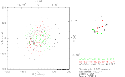
Figure 3: 4 AT $\times$ 3 night configuration (left). 6 AT $\times$ 1 night configuration (right).

• 4 UTs $\times$ 1 night (U1-U2-U3-U4) –- faint source configuration (Fig. 2);

• 4 ATs $\times$ 3 nights (A0-B1-D2-G1, D1-E0-H0-J3, A0-G0-I1-M0) –- the minimum imaging $uv$ coverage consistent with the current VLTI capabilities (Fig. 3; left);

• 6 ATs $\times$ 1 night (A0-B1-D2-G1-J2-M0) –- a 6 telescope extended configuration with one night observation; has less uv points than the 4 AT x 3 nights configuration (Fig. 3; right).

3 Noise Model

The noise model estimates the uncertainties on squared visibilities and closure phases assuming an instrument following a multi-axial recombination scheme with a fringe tracker (FT; Jocou et al.2007).

The quantity we procure is the total number of detected photoevents per baseline in 5 minutes in the photometric channel:

$N_{p}=\frac{N_{total}\times(1-f)\times 5\times N_{obs}}{N_{base}}$

where $f$ is the fraction of the beam that gores into the interferometric channel (90%), $N_{obs}$ is the number of observations per minute, $N_{base}$ is the number of baselines and $N_{total}$ is the total number of detected photevents per integration point in all channels:

$N_{total}=F_{0}\times 10^{-0.4mag}\times t_{int}\times N_{tel}\times\pi\times R^{2}\times\Delta\lambda\times trans\times Strehl$

Here $F_{0}$ is the photon flux of a zeroth magnitude star (Jocou et al. 2007), $mag$ is the object magnitude in the observing band, $t_{int}$ is the integration time (0.05 s), $N_{tel}$ is the number of telescopes (6 or 4), $R$ is the radius of the telescopes (4.1 for UTs and 0.9 for ATs) assumed for simplification to have no central hole, $\Delta\lambda$ is the spectral bandwidth (chosen), $trans$ is the total instrument transmission including quantum efficiency (Jocou et al. 2007), and $Strehl$ is the Strehl ratio and depends on wavelength (Jocou et al. 2007).

The correlated flux per baseline is given by:

$F_{cor}=\frac{N_{i}\times V^{\prime}}{2}$

where $V^{\prime}$ is the instrumental visibility loss (80%) and FT loss (90%) corrected visibility and $N_{i}=N_{total}\times f\times 5\times N_{obs}/N_{base}$, is the detected number of photoevents per baseline in 5 minutes in the interferometric channel.

The signal-to-noise ratio of the squared correlated flux ($SNR$) is a complex function of $F_{cor}$, $N_{i}$, $V^{\prime}$, $N_{tel}$, $N_{pix}$ the number of pixels needed to code the interferometric channel (600) and $\sigma$ the detector readout noise (15 e-).

Therefore, the uncertainty on the squared visibility is:

$error_{V^{2}}=V^{\prime 2}\times{\sqrt{SNR^{-2}+2\times(N_{p}+N_{pixp}\,\sigma^{2}/N_{p}^{2})}}$

where $N_{pixp}$ is the number of pixels needed to code the photometric channel (4).

The photon noise on the closure phase ($Phot$) is a function of $N_{tel}$, $N_{i}$, $V_{123}$, $V_{1}$, $V_{2}$, $V_{3}$, $V_{12}$, $V_{23}$, $V_{13}$, where the $V$ terms correspond to visibilities in a combination of one, two or three telescopes. The detector noise on the closure phase ($Det$) depends on $N_{tel}$, $N_{i}$, $N_{pix}$, $\sigma$ and the $V$ terms.

Therefore, the total noise on the closure phase is estimated as:

$error_{T}=\sqrt{\frac{Phot+Det}{5\times N_{obs}}}$

4 OIFITS File Generation

The advent of optical interferometry has lead to the need for a common data format based on the Flexible Image Transport System (FITS) in order to facilitate data reduction and the combination of various types of interferometer data. The result was the creation of the OI Exchange Format or OIFITS format (Pauls et al. 2004). Interferometer projects supporting this standard include COAST, NPOL, IOTA, VLTI, PTI and the Keck Interferometer.

OIFITS format is designed so that different categories of information are stored in distinct “tables” within a file and can be cross-referenced one to another. Each OIFITS file “table” stores specific parameters that include interferometric observables –- complex visibility (OI-VIS), squared visibilities (OI-VIS2), and the triple product (bispectrum/closure phase; OI-T3) –- and ancillary data like Universal Time measurements, spectral bandpass and wavelengths (OI-WAVELENGTH), target identification (OI-TARGET) and telescope coordinates (OI-ARRAY).

Synthetic images were provided by the science case groups (Garcia et al. 2007) and imported into aspro, an image simulation tool originally created for IRAM. Assuming the objects were located at a $-$60 degree declination angle, typical object magnitudes were used to generate noisy, squared visibilities and closure phases. We assumed an one hour per calibrated measurement. The actual on-source integration time is, however, 10-15 minutes per hour due to overheads. The total integration time assumes an entire transit (9 hours).

5 Phase Closure Theory

Figure 4:

Given an incoherent source, the observed brightness distribution in a direction $\vec{s^{\prime}}$ is given by (Fig. 4):

$I^{obs}(\vec{s^{\prime}})=I^{obs}(x,y)=PSF(x,y)*I^{true}(x,y)+N(x,y)$

where PSF(x,y) is the point spread function, I^true(x,y) is the true object brightness distribution, N(x,y) is the noise and the asterisk denotes convolution.

In practice, interferometry does not make measurements in the image plane but in Fourier space. The relevant quantity is called the complex visibility and is measured at each uv point, the position vector of the baseline on a plane perpendicular to the source direction:

$V^{obs}(u,v)=V^{true}(u,v)\times S(u,v)+N^{\prime}(u,v)$

where S(u,v), the sampling function, is the Fourier transform of the PSF(x,y), V^true(x,y), the true visibility, is the Fourier transform of the true brightness distribution I^true(x,y) and N’(u,v) is the noise in the Fourier space.

The van Cittert-Zernike theorem states that the true brightness distribution can be obtained by the inverse Fourier transform and deconvolution of the observables:

$I^{true}(x,y)*PSF(x,y)=\int\int V^{true}(u.v)\times S(u,v)\,exp\,[2\pi i(ux+vy)]\,du\,dv$

The role of image reconstruction is to obtain the best approximation, I^aprox(x,y) $\sim$ I^true(x,y), to the true brightness distribution. For phase closure image reconstruction we want to find a solution which has the maximum probability given the data. The solution I^aprox(x,y) involves minimizing the value of a penalty term subject to some condition:

$P(z)=P_{L}(z)+P_{prior}(z)=P_{L}(z)+\mu R(z)$

where z represents the intensity of the pixels, P_L is the likelihood penalty, $P_{prior}$ is the prior penalty, R(z) is the regularization term and $\mu$ is a multiplier (hyperparameter) tuned so that at the solution, the likelihood terms are equal to their expected values. P_L enforces agreement with the data, while P_prior provides information where the data fail to do so, in particular in regions where the noise dominates or where the data are missing. P_prior is responsible for the so-called regularization of the inverse problem.

The solution is therefore found by minimizing the likelihood penalty term for squared visibilities and triple products under a prior constraint:

$P_{L}=P_{V^{2}}P_{T}\propto-\exp{\frac{\chi^{2}_{V^{2}}+\chi^{2}_{T}}{2}}$

where $\chi^{2}_{V^{2}}$ is the likelihood term with respect to the squared visibility data and $\chi^{2}_{T}$ to the triple product. Typically, the data penalties are defined assuming the measurements follow Gaussian statistics:

$$\chi^{2}_{V^{2}}(z)=\sum\frac{1}{\sigma^{2}_{V^{2}}}\,\left(V^{2}_{\mathrm{data}}-V^{2}_{\mathrm{model}}\right)^{2}$$

$$\chi^{2}_{\mathrm{T}}(z)=\sum\frac{1}{\sigma^{2}_{\mathrm{T}}}\,\left|\mathrm{e}^{\mathrm{i}\,\phi^{\mathrm{data}}_{\mathrm{T}}}-\mathrm{e}^{\mathrm{i}\,(\varphi_{1}+\varphi_{2}-\varphi_{3})}\right|^{2}$$

where V² refers to the squared visibilities (data and model), $\phi_{T}^{data}$ to the measured closure phase, $\varphi_{1}$, $\varphi_{2}$, $\varphi_{3}$ to three individual phases involved in the phase closure and $\sigma$ to the respective standard deviations.

Regularization can enforce agreement with some preferred and/or exact properties of the solution. Because we want to favor compact sources, smoothness is a very common regularization constraint:

$R(z)=\sum\,w\,|z|^{2}$

where the regularization weights w are chosen in order to ensure spectral smoothing, that is, it enforces smoothness of the Fourier spectrum of the image and enforces compactness of the brightness distribution of the field of view.

We have implemented the Multi-Aperture Reconstruction Algorithm (mira; version 0.7; April 2008) as developed by Eric Thiebaut with support from the Jean-Marie Mariotti Center (JMMC). mira works in the yorick and C platform and is optimized to handle optical interferometric data with sparse uv coverage (Thiebaut 2005). Typically, mira implements several types of regularization of which smoothness and maximum entropy are some examples.

6 Image Analysis

Because mira typically superresolves in the image reconstruction, we have compared our reconstructed images with the synthetic images provided by the science groups. Relative astrometry information was obtained for the images using ds9. Photometry of the image components was performed using iraf procedure phot. $SNR_{V^{2}}$ and $SNR_{T}$ correspond to the range of signal-to-noise ratios in the squared visbilities and closure phases measured in the synthetic images.

7 Closure Phase Image Reconstruction

Figure 5: A simulated AGN with torus, 0.1 mas/pixel sampling; mira reconstruction 4 UT $\times$ 1 night configuration, smoothness regularization, 0.1 mas/pixel sampling.

Table 1: AGN. Diameter units are in pixels.

	Image	mira 4 UT
flux nucleus	22.3%	-
flux inner diameter	55.0%	-
flux outer diameter	17.6%	91.6%
flux torus	5.1%	8.4%
nuclear diameter	7	-
inner diameter	30	-
outer diameter	75	70
torus diameter	260	-
SNR${}_{V^{2}}$	-	553-704
SNRT	-	0.3-0.4

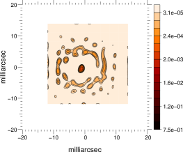
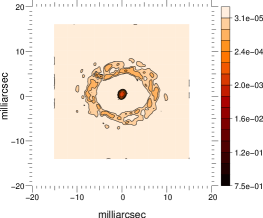
Figure 6: A low mass evolved star system with an outflow, 0.1 mas/pixel sampling; mira reconstruction 4 AT $\times$ 3 nights configuration, smoothness regularization, 0.1 mas/pixel sampling; mira reconstruction 6 AT $\times$ 1 night configuration, smoothness regularization, 0.1 mas/pixel sampling.

Table 2: Evolved Star. Diameter units are in pixels.

	Image	mira 4 AT 3	mira 6 AT
flux star	25.1%	22.3%	22.5%
flux wind	74.9%	77.7%	77.5%
ratio star/wind	0.3	0.3	0.3
star diameter	10	15	12
inner wind diameter	60 $\times$ 40	50 $\times$ 30	60 $\times$ 40
outer wind diameter	100 $\times$ 80	90 $\times$ 80	100 $\times$ 80
SNR${}_{V^{2}}$	-	63-2336	38-1706
SNRT	-	0.01-0.2	1.0-44

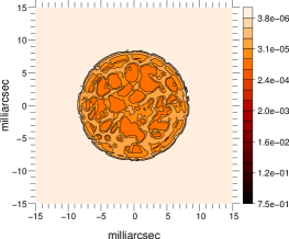
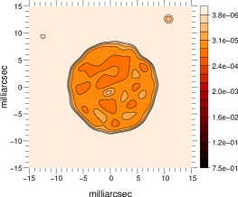
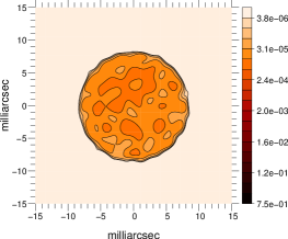
Figure 7: A simulated stellar surface of a M giant, 0.1 mas/pixel sampling; mira reconstruction 4 AT $\times$ 3 nights configuration, smoothness regularization, 0.1 mas/pixel sampling, SNR${}_{v^{2}}$=1.5-541, SNR_T=0.01-05; mira reconstruction 6 AT $\times$ 1 night configuration, smoothness regularization, 0.1 mas/pixel sampling, SNR${}_{V^{2}}$=0.1-600, SNR_T=0.1-115.

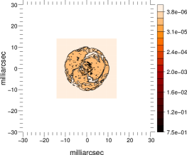
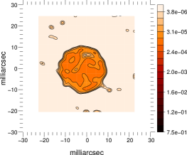
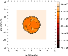
Figure 8: A simulated stellar surface of a supergiant, 0.1 mas/pixel sampling; mira reconstruction 4 AT $\times$ 3 nights configuration, smoothness regularization, 0.1 mas/pixel sampling, SNR=${}_{V^{2}}$=4-4900, SNR_T= 0.004-0.09; mira reconstruction 6 AT $\times$ 1 night configuration, smoothness regularization, 0.1 mas/pixel sampling, SNR${}_{V^{2}}$=4-2999, SNR_T=0.2-116.

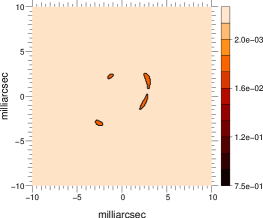
Figure 9: A simulated microlensing event, 0.1 mas/pixel sampling; mira reconstruction 4 UT $\times$ 1 night configuration, smoothness regularization, 0.1 mas/pixel sampling.

Table 3: Microlensing. Distance is in pixels.

	Image	mira 4 UT
A flux	19.6%	19.6%
B flux	11.9%	11.9%
C flux	29.8%	29.8%
D flux	38.7%	38.7%
ratio D/A	2.0	2.0
ratio D/B	3.3	3.3
ratio D/C	1.3	1.3
distance AB	40	40
distance BC	20	20
distance CD	56	56
SNR${}_{V^{2}}$	-	228-268
SNRT	-	0.1-0.4

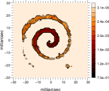
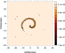
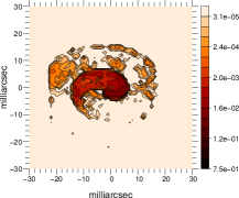
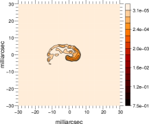
Figure 10: A simulated image of the pinwheel nebula at 0 degree inclination, 1.0 mas/pixel sampling; mira reconstruction 6 AT $\times$ 1 night configuration, smoothness regularization. A simulated iamge of the pinwheel nebula at 60 degree inclination, 1.0 mas/pixel sampling; mira reconstruction 6 AT $\times$ 1 night configuration, smoothness regularization, 0.1 mas/pixel sampling.

Table 4: Pinwheel

	Angle	Image	SNR${}_{V^{2}}$	SNRT	mira 6 AT
inner spiral	0 deg	100 $\times$ 80	49-861	2-19	100 $\times$ 80
inner spiral	60 deg	100 $\times$ 60	36-861	1-43	100 $\times$ 60

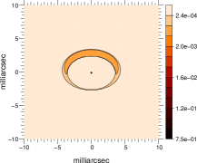
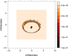
Figure 11: A simulated stellar surface of the structure of inner disks surrounding YSOs, 0.1 mas/pixel sampling; mira reconstruction 4 UT $\times$ 1 night configuration, smoothness regularization, 0.1 mas/pixel sampling; mira reconstruction 4 AT $\times$ 3 nights configuration, smoothness regularization, 0.1 mas/pixel sampling; mira reconstruction 6 AT $\times$ 1 night configuration, smoothness regularization, 0.1 mas/pixel sampling.

Table 5: YSO. Radii units are in pixels.

	Image	mira 4 UT	mira 4 AT 3	mira 6 AT
flux star	18.1%	18.7%	18.6%	18.6%
flux disk	81.9%	81.3%	81.4%	81.4%
ratio	0.2	0.2	0.2	0.2
inner diameter	65 $\times$ 45	65 $\times$ 45	65 $\times$ 45	65 $\times$ 45
outer diameter	85 $\times$ 60	80 $\times$ 56	82 $\times$ 60	85 $\times$ 60
SNR${}_{V^{2}}$	-	2055-5215	89-1385	12-1363
SNRT	-	0.04-0.2	0.04-0.5	0.2-12

8 Discussion

8.1 The Sources

In general, the image reconstruction faired very well. This is denoted by the excellent astrometry and photometry of the individual image elements. Some sources merit a separate discussion.

We are able to detect the unresolved AGN out to the sublimation radius. The total flux contained in this region is 91.6% compared to the 91.4% measured in the synthetic image. The result suggests that such observations will provide important constraints on the size of the sublimation region and torus in the nearest AGN.

For the stellar surfaces, our results show unprecedented detail. Most of the flux is recovered in a compact region and careful inspection of the reconstructed images shows correspondence with individual regions of different brightness in the synthetic image. The edges of the stellar surface are also well reproduced.

8.2 Number of Telescopes and $uv$ Coverage

Our results show that the use of the 6 AT $\times$ 1 night configuration generally yields better reconstructed images than the 4 AT $\times$ 3 nights configuration, even though the number of $uv$ points is similar. This is particularly noted in images of stellar surfaces and in stellar disks/winds. This is in consonance with previous studies (Tuthill & Monnier 2000; Baron 2007). The image reconstruction result is satisfactory with a low number of array elements when the source is compact (Tuthill & Monnier 2000). However, when the sources are more complex, a larger Fourier plane coverage is needed and therefore more array elements are needed.

Indeed it is the number of telescopes and not the number of observing nights (and therefore total number of $uv$ points) that determine the image reconstruction outcome. In a system of N telescopes, the number of uv points is $\frac{1}{2}N\times(N-1)$ per night per integration point and the number of independent closure phases is $\frac{1}{2}$ $\times$ (N-1) $\times$ (N-2) per night per integration point. With N=4 and 3 nights, for each integration point there are a total of 18 $uv$ points (therefore squared visibilities) and a total of 9 closure phases. For N=6 and 1 night, the number of squared visibilities and closure phases per integration point is 15 and 10, respectively.

On the other hand, the image reconstruction (or fitting process) can only make use of the instantaneous phases to create a model brightness. Therefore, for a N=4 system, the image reconstruction uses the 3 instantaneous closure phases (3 per night), while with 6 telescopes there are now 10 independent closure phases.

8.3 Dynamic Range

Image reconstruction, whatever the method, is crucial when a high dynamic range ($>$1000) is required. Our results show that the closer phase technique allows to achieve modest dynamic ranges. Higher dynamic ranges can be obtained by using the VLTI coupled with a phase referencing instrument, like PRIMA (Deplanke et al. 2000) which will allow to reach K band magnitudes of 11 mag for the ATs and 14 mag for the UTs. The presence of nearby phase referencing sources will allow larger integration times on source and therefore higher dynamic range.

9 Conclusions

Next generation optical interferometric instrumention like the VSI will be designed to offer superb imaging capabilities in order to bypass ambiguities in the interpretation of visibility data. It will be particularly novel in that it will allow spatial resolutions of milliarcseconds, comparable to ALMA and even better the future JWST.

In order to test future VLTI performance in terms of imaging, we have run several tests on key scientific cases. Results show that with a simple 6 Auxiliary Telescope (AT) configuration and 1 night observation, images of high image fidelity can be obtained. Using the VLTI alone will allow to achieve modest dynamic ranges, although in conjunction with a phase referencing instrument, K band magnitudes of 11 and 14 mag can be reached with the ATs and UTs, respectively. Such diverse objects as AGN, stellar surfaces and disks are shown possible to image with future VLTI instumentation.

10 Acknowledgments

MEF is supported by the Funda cão para a Ciência e a Tecnologia through the research grant SFRH/BPD/36141/2007. PJVG and MEF were supported in part by the Funda cão para a Ciência e a Tecnologia through projects PTDC/CTE-AST/68915/2006 and PTDC/CTE-AST/65971/2006 from POCI, with funds from the European programme FEDER.

11 References

Baron, F., 2007, bsmem Test Plan Results, private communication

Deplancke, F. et l. 2000, SPIE, 4006, 365

Garcia, P. et al. 2007, in doc. VLT-SPE-VSI-15870-4335, issue 1.0 in VSI Phase A Document Package, Science Cases

Hofmann, K. -H. & Weigelt, G. 1993, A&A, 278, 328

Jocou, L. et al. 2007, in doc. VLT-SPE-VSI-15870-4335, issue 1.0 in VSI Phase A Document Package, System Design

Lopez, B., et al. 2006, in Advances in Stellar Interferometry, Editted by Monnier, John D., Schöller, Marcus, Danchi, William C., Proceedings of SPIE, 6268, 31

Malbet, F., et al. 2006, in doc. VSI-PRO-001, issue 1.0, VSI Technical Proposal in Response to ESO Call for Phase A Proposals for 2nd Generation VLTI Instruments

Masoni, L. 2006, PADEU, 17, 155

Masoni, L. et al. 2005, Astr. Nachr., 326, 566

Pauls, Young, Cotton & Monnier 2004, Chara Technical Report

Thiebaut, E., 2005, Optics in Astrophysics: Proceedings of the NATO advanced Study Institute on Optics in Astrophysics, Cargese, France, vol 198, eds. R. Foy & F. -C. Foy, pg. 397

Tuthill, P. G. & Monnier, J. D., 1 August 2000, Chara Technical Report, no. 86

Weigelt, G., Balega, Y., Bloecker, T., Fleischer, A. J., Osterbart, R., & Winter, J. M. 1998, A&A, 333, L51