Quantum Monte Carlo calculations of magnetic moments and $\bm{M}$1 transitions in $\bm{A\leq 7}$ nuclei including meson-exchange currents

Abstract

Green’s function Monte Carlo calculations of magnetic moments and $M1$ transitions including two-body meson-exchange current (MEC) contributions are reported for $A\leq 7$ nuclei. The realistic Argonne $v_{18}$ two-nucleon and Illinois-2 three-nucleon potentials are used to generate the nuclear wave functions. The two-body meson-exchange operators are constructed to satisfy the continuity equation with the Argonne $v_{18}$ potential. The MEC contributions increase the $A$=3,7 isovector magnetic moments by 16% and the $A$=6,7 $M1$ transition rates by 17–34%, bringing them into very good agreement with the experimental data.

I Introduction

In a recent paper PPW07 we reported quantum Monte Carlo (QMC) calculations of electroweak transitions in $A=6,7$ nuclei. The QMC method is a two-step process, with an initial variational Monte Carlo (VMC) calculation to find a good trial function, followed by a Green’s function Monte Carlo (GFMC) calculation to refine the solution. When used with the Argonne $v_{18}$ two-nucleon WSS95 ($N\!N$) and Illinois-2 three-nucleon PPWC01 ($3N$) potentials, the final GFMC results reproduce the ground- and excited-state energies for $A\leq 10$ nuclei PW01 ; PVW02 ; PWC04 ; P05 very well.

In Ref. PPW07 we studied magnetic dipole ($M1$) and electric quadrupole ($E2$) transitions and nuclear beta-decay (Fermi and Gamow-Teller) rates. These were the first off-diagonal matrix element calculations using the nuclear GFMC method. However, only one-body transition operators were used to calculate the matrix elements. We noted that two-body meson-exchange-current (MEC) operators are known to increase isovector magnetic moments by 15-20% for $A$=3 nuclei Car98 , while a previous VMC calculation for the width of the first $M1$ transition in ⁶Li was also increased by 20% WS98 . In this paper we use GFMC wave functions to investigate MEC contributions to magnetic moments for the ground states of $A$=2–7 nuclei as well as a number of $M1$ transitions in $A$=6,7 nuclei. We find significant isovector contributions from the MEC operators and overall very good agreement with experiment.

A brief review of the QMC calculational method is given in Sec. II. The electromagnetic current operator is discussed in detail in Sec. III. Results and conclusions are given in Secs. IV and V.

II Quantum Monte Carlo method for transitions

We evaluate the diagonal magnetic moment matrix element $\langle\Psi(J^{\pi};T)|{\cal O}|\Psi(J^{\pi};T)\rangle$ and the off-diagonal transition matrix element $\langle\Psi_{f}(J^{\pi^{\prime}};T^{\prime})|{\cal O}|\Psi_{i}(J^{\pi};T)\rangle$, where $\cal O$ is the full electromagnetic operator. The nuclear wave function with a specific spin-parity $J^{\pi}$ and isospin $T$ is denoted as $\Psi(J^{\pi};T)$ and is a solution of the many-body Schrödinger equation

$$H\Psi(J^{\pi};T)=E\Psi(J^{\pi};T)\ .$$ (1)

The Hamiltonian used here has the form

$$H=\sum_{i}K_{i}+{\sum_{i<j}}v_{ij}+\sum_{i<j<k}V_{ijk}\ ,$$ (2)

where $K_{i}$ is the nonrelativistic kinetic energy and $v_{ij}$ and $V_{ijk}$ are respectively the Argonne $v_{18}$ (AV18) WSS95 and Illinois-2 (IL2) PPWC01 potentials. The VMC trial function $\Psi_{T}(J^{\pi};T)$ for a given nucleus is constructed from products of two- and three-body correlation operators acting on an antisymmetric single-particle state of the appropriate quantum numbers. The correlation operators are designed to reflect the influence of the interactions at short distances, while appropriate boundary conditions are imposed at long range W91 ; PPCPW97 . The $\Psi_{T}(J^{\pi};T)$ has embedded variational parameters that are adjusted to minimize the expectation value

$$E_{V}=\frac{\langle\Psi_{T}|H|\Psi_{T}\rangle}{\langle\Psi_{T}|\Psi_{T}\rangle}\geq E_{0}\ ,$$ (3)

which is evaluated by Metropolis Monte Carlo integration MR2T2 . Here $E_{0}$ is the exact lowest eigenvalue of $H$ for the specified quantum numbers. A good variational trial function has the form

$$|\Psi_{T}\rangle=\left[1+\sum_{i<j<k}\widetilde{U}^{TNI}_{ijk}\right]\left[{\cal S}\prod_{i<j}(1+U_{ij})\right]|\Psi_{J}\rangle\ .$$ (4)

The Jastrow wave function, $\Psi_{J}$, is fully antisymmetric and has the $(J^{\pi};T)$ quantum numbers of the state of interest, while $U_{ij}$ and $\tilde{U}^{TNI}_{ijk}$ are the two- and three-body correlation operators. More details may be found in Ref. PPW07 . The error in the variational energy $E_{V}$ is of order $|\Psi_{0}-\Psi_{T}|^{2}/|\Psi_{T}|^{2}$, where $\Psi_{0}$ is the exact lowest-energy eigenstate of $H$ for a given set of quantum numbers. Other expectation values calculated with $\Psi_{T}$ have errors of order $|\Psi_{0}-\Psi_{T}|/|\Psi_{T}|$.

The GFMC method C87 ; C88 reduces the VMC errors by using the relation

$$\Psi_{0}=\lim_{\tau\rightarrow\infty}\exp[-(H-E_{0})\tau]\Psi_{T}\ ;$$ (5)

that is the operator $\exp[-(H-E_{0})\tau]$ projects $\Psi_{0}$ out of $\Psi_{T}$. If the maximum $\tau$ actually used is large enough, the eigenvalue $E_{0}$ is calculated exactly while other expectation values are generally calculated neglecting terms of order $|\Psi_{0}-\Psi_{T}|^{2}/|\Psi_{T}|^{2}$ and higher PPCPW97 .

In the following we present a brief overview of the nuclear GFMC method; much more detail may be found in Refs. PPCPW97 ; WPCP00 . We start with the $\Psi_{T}$ of Eq. (4) and define the propagated wave function $\Psi(\tau)$

$$\Psi(\tau)=e^{-({H}-E_{0})\tau}\Psi_{T}=\left[e^{-({H}-E_{0})\triangle\tau}\right]^{n}\Psi_{T}\ ,$$ (6)

where we have introduced a small time step, $\tau=n\triangle\tau$; obviously $\Psi(\tau=0)=\Psi_{T}$ and $\Psi(\tau\rightarrow\infty)=\Psi_{0}$. Quantities of interest are evaluated in terms of a “mixed” expectation value between $\Psi_{T}$ and $\Psi(\tau)$:

$$\langle O(\tau)\rangle_{M} = \frac{\langle\Psi(\tau)|O|\Psi_{T}\rangle}{\langle\Psi(\tau)|\Psi_{T}\rangle}.$$ (7)

The desired expectation values would, of course, have $\Psi(\tau)$ on both sides; by writing $\Psi(\tau)=\Psi_{T}+\delta\Psi(\tau)$ and neglecting terms of order $[\delta\Psi(\tau)]^{2}$, we obtain the approximate expression

$$\langle O(\tau)\rangle=\frac{\langle\Psi(\tau)|O|\Psi(\tau)\rangle}{\langle\Psi(\tau)|\Psi(\tau)\rangle}\approx\langle O(\tau)\rangle_{M}+[\langle O(\tau)\rangle_{M}-\langle O\rangle_{V}]~{},$$ (8)

where $\langle O\rangle_{\rm V}$ is the variational expectation value.

For off-diagonal matrix elements relevant to this work the generalized mixed estimate is given by the expression

$$\frac{\langle\Psi^{f}(\tau)|O|\Psi^{i}(\tau)\rangle}{\sqrt{\langle\Psi^{f}(\tau)|\Psi^{f}(\tau)\rangle}\sqrt{\langle\Psi^{i}(\tau)|\Psi^{i}(\tau)\rangle}}\approx\langle O(\tau)\rangle_{M_{i}}+\langle O(\tau)\rangle_{M_{f}}-\langle O\rangle_{V}\ ,$$ (9)

where

$$\langle O(\tau)\rangle_{M_{i}} = \frac{\langle\Psi^{f}_{T}|O|\Psi^{i}(\tau)\rangle}{\langle\Psi^{i}_{T}|\Psi^{i}(\tau)\rangle}\sqrt{\frac{\langle\Psi^{i}_{T}|\Psi^{i}_{T}\rangle}{\langle\Psi^{f}_{T}|\Psi^{f}_{T}\rangle}}\ ,$$ (10)

and $\langle O(\tau)\rangle_{M_{f}}$ is defined similarly. For more details see Eqs. (19-24) and the accompanying discussions in Ref. PPW07 .

III The electromagnetic current operator

The model used for the nuclear electromagnetic current operator ${{\bm{j}}}({{\bm{q}}})$ is based on the study of Ref. Mar05 . It represents ${{\bm{j}}}({{\bm{q}}})$ as a sum of one-, two- and three-body terms that operate on the nucleon degrees of freedom,

$${\bm{j}}({\bm{q}})=\sum_{i}{\bm{j}}_{i}({\bm{q}})+\sum_{i<j}{\bm{j}}_{ij}({\bm{q}})+\sum_{i<j<k}{\bm{j}}_{ijk}({\bm{q}})\ ,$$ (12)

${{\bm{q}}}$ being the three-momentum transfer. The one-body operator ${{\bm{j}}}_{i}({{\bm{q}}})$ is derived from the nonrelativistic reduction of the covariant single-nucleon current, by expanding in inverse powers of the nucleon mass $m$. In the notation of Ref. Car98 , it is written as

$${\bm{j}}_{i}({\bm{q}})=\frac{\epsilon_{i}}{2m}\{{\bm{p}}_{i},{\rm e}^{{\rm i}{\bm{q}}\cdot{\bm{r}}_{i}}\}+\frac{\rm i}{2m}\mu_{i}{\bm{\sigma}}_{i}\times{\bm{q}}\,{\rm e}^{{\rm i}{\bm{q}}\cdot{\bm{r}}_{i}}\ ,$$ (13)

where $\{\cdots,\cdots\}$ denotes the anticommutator, the quantities $\epsilon_{i}$ and $\mu_{i}$ are defined as

$$\epsilon_{i} = \frac{1}{2}\left[G_{E}^{S}(q_{\mu}^{2})+G_{E}^{V}(q_{\mu}^{2})\tau_{i,z}\right]\ ,$$ (14)

$$\mu_{i} = \frac{1}{2}\left[G_{M}^{S}(q_{\mu}^{2})+G_{M}^{V}(q_{\mu}^{2})\tau_{i,z}\right]\ ,$$ (15)

and ${\bm{p}}$, ${\bm{\sigma}}$ and ${\bm{\tau}}$ are the nucleon’s momentum, Pauli spin and isospin operators, respectively. Finally, $G_{E}^{S}(q_{\mu}^{2})$ ($G_{M}^{S}(q_{\mu}^{2})$) and $G_{E}^{V}(q_{\mu}^{2})$ ($G_{M}^{V}(q_{\mu}^{2})$) are the isoscalar and isovector combinations of the nucleon electric (magnetic) Sachs form factors, respectively, evaluated at the four-momentum transfer $q_{\mu}^{2}=q^{2}-\omega^{2}$ with $\omega=\sqrt{q^{2}+M_{f}^{2}}-M_{i}$, where $M_{i}$ and $M_{f}$ are initial and final nuclear masses (only elastic scattering or inelastic scattering to discrete final states are considered in the present work).

The current operator satisfies the current conservation relation (CCR)

$${{\bm{q}}}\cdot{{\bm{j}}}({{\bm{q}}})=[H,\rho({{\bm{q}}})]\ .$$ (16)

Here $H$ is the nuclear Hamiltonian consisting of two- and three-nucleon interactions, the AV18 WSS95 and IL2 PPWC01 potentials, respectively, and $\rho({\bm{q}})$ is the charge operator which, to lowest order in $1/m$, is written as

$$\rho({\bm{q}})=\sum_{i}\rho_{i}({\bm{q}})\ ,$$ (17)

with

$$\rho_{i}({\bm{q}})=\epsilon_{i}\,{\rm e}^{{\rm i}{\bm{q}}\cdot{\bm{r}}_{i}}\ .$$ (18)

To this order, the CCR separates into

$${{\bm{q}}}\cdot{{\bm{j}}}_{i}({{\bm{q}}}) = \biggl{[}{{{\bm{p}}}_{i}^{2}\over 2m},\rho_{i}({{\bm{q}}})\biggr{]}\ ,$$ (19)

$${{\bm{q}}}\cdot{{\bm{j}}}_{ij}({{\bm{q}}}) = [v_{ij},\rho_{i}({{\bm{q}}})+\rho_{j}({{\bm{q}}})]\ ,$$ (20)

and similarly for the three-body current ${{\bm{j}}}_{ijk}({{\bm{q}}})$. The one-body current of Eq. (13) is easily seen to satisfy Eq. (19).

III.1 Two-nucleon current

The two-body current operator ${{\bm{j}}}_{ij}({{\bm{q}}})$ is separated into two parts, labeled model-independent (MI) and model-dependent (MD), following the scheme of Ref. Ris89 . The MI two-body currents have longitudinal components that satisfy the CCR of Eq. (20) with the $N\!N$ potential $v_{ij}$, i.e. the AV18 WSS95 . The potential can be written as

$$v_{ij}=v^{IC}_{ij}+v^{IB}_{ij}\ ,\qquad v^{IC}_{ij}=v^{0}_{ij}+v^{p}_{ij}\ ,$$ (21)

where $v_{ij}^{IC}$ and $v_{ij}^{IB}$ are the isospin-symmetry conserving ($I$$C$) and breaking ($I$$B$) parts of the potential, respectively, and $v_{ij}^{0}$ and $v_{ij}^{p}$ are the momentum-independent and momentum-dependent parts of the interaction. For the AV18, $v_{ij}^{0}$ corresponds to the contributions of the static components, including isospin-independent and isospin-dependent central, spin-spin, and tensor terms, while $v_{ij}^{p}$ retains the contributions from the spin-orbit and quadratic momentum-dependent components. The $v_{ij}^{IB}$ part in the AV18 is parameterized by the four operators

$$O^{p=15,\ldots,18}_{ij}=T_{ij}\>\>\>,\,{\bm{\sigma}}_{i}\cdot{\bm{\sigma}}_{j}T_{ij}\>\>\>,\,S_{ij}\,T_{ij}\>\>\>,\,(\tau_{i,z}+\tau_{j,z})\ ,$$ (22)

where $S_{ij}$ is the standard tensor operator and the isotensor operator $T_{ij}$ is defined as $T_{ij}=3\,\tau_{i,z}\,\tau_{j,z}-{\bm{\tau}}_{i}\cdot{\bm{\tau}}_{j}$.

The MI two-body currents arising from $v_{ij}^{0}$ have been constructed following the procedure of Ref. Ris85 , which will be hereafter referred to as the meson-exchange (ME) scheme. Within this scheme, the isospin-dependent static part of $v_{ij}^{0}$ is assumed to be induced by exchanges of effective pseudoscalar (PS), or “$\pi$-like,” and vector (V), or“$\rho$-like,” mesons. The propagators associated with these exchanges are projected out of the (isospin-dependent) central, spin-spin, and tensor components of $v_{ij}^{0}$. The resulting two-body currents satisfy the CCR with $v_{ij}^{0}$ by construction. Explicit expressions can be found in a number of references (see Ref. Mar05 and references therein).

The currents arising from $v_{ij}^{p}$ have been obtained following the procedure of Ref. Sac48 , which will be referred to as the minimal-substitution (MS) scheme, reviewed and generalized in Ref. Mar05 . We first note that the isospin operator ${\bm{\tau}}_{i}\cdot{\bm{\tau}}_{j}$ can be expressed in terms of the space-exchange operator ($P_{ij}$), using the relation

$${\bm{\tau}}_{i}\cdot{\bm{\tau}}_{j}=-1-(1+{\bm{\sigma}}_{i}\cdot{\bm{\sigma}}_{j})P_{ij}\ ,$$ (23)

valid when operating on antisymmetric wave functions. The operator $P_{ij}$ is defined as $P_{ij}={\rm e}^{{{\bm{r}}}_{ji}\cdot{{\bm{\nabla}}}_{i}+{{\bm{r}}}_{ij}\cdot{{\bm{\nabla}}}_{j}}$, where the ${{\bm{\nabla}}}$-operators do not act on the vectors ${{\bm{r}}}_{ij}={{\bm{r}}}_{i}-{{\bm{r}}}_{j}=-{{\bm{r}}}_{ji}$ in the exponential. In the presence of an electromagnetic field, minimal substitution is performed both in the explicit momentum dependence of the two-nucleon potential as well as in the implicit momentum dependence implied by ${\bm{\tau}}_{i}\cdot{\bm{\tau}}_{j}$. The resulting current operators have been derived in Ref. Mar05 . Here we only list the final result for the current operators associated with the isospin-independent and isospin-dependent spin-orbit interaction. In this case, $v_{ij}^{p}$ can be expressed as

$$v_{ij}^{p}=v_{1,ij}^{p}+v_{2,ij}^{p}{\bm{\tau}}_{i}\cdot{\bm{\tau}}_{j}\ ,$$ (24)

where

$$v^{p}_{1,ij} = v_{ls}(r)\,{\bm{L}}\cdot{\bm{S}}\ ,$$

$$v^{p}_{2,ij} = v_{ls\tau}(r)\,{\bm{L}}\cdot{\bm{S}}\ ,$$ (25)

with ${\bm{L}}={\bm{r}}_{ij}\times({{\bm{p}}}_{i}-{{\bm{p}}}_{j})/2$, and ${\bm{S}}$ is the total spin of pair $ij$ and $v_{ls}$ and $v_{ls\tau}$ are the spin-orbit parts of the $N\!N$ potential. Performing minimal substitution in $v^{p}_{1}$, we obtain

$${\bm{j}}_{ij}({\bm{q}};ls)=\frac{1}{2}v_{ls}(r)\biggl{(}\epsilon_{i}\,{\rm e}^{{\rm i}{\bm{q}}\cdot{\bm{r}}_{i}}-\epsilon_{j}\,{\rm e}^{{\rm i}{\bm{q}}\cdot{\bm{r}}_{j}}\biggr{)}\,{\bm{S}}\times{\bm{r}}_{ij}\ .$$ (26)

For the isospin-dependent term $v^{p}_{2}$, we first symmetrize it as

$$v^{p}_{2,ij}\,{\bm{\tau}}_{i}\cdot{\bm{\tau}}_{j}=\frac{1}{2}v_{ls\tau}(r)\left({\bm{L}}\cdot{\bm{S}}\,{\bm{\tau}}_{i}\cdot{\bm{\tau}}_{j}+{\bm{\tau}}_{i}\cdot{\bm{\tau}}_{j}\,{\bm{L}}\cdot{\bm{S}}\right)\ ,$$ (27)

and the associated current then reads

$${\bm{j}}_{ij}({\bm{q}};ls\tau) = \frac{1}{4}v_{ls\tau}(r){\bm{S}}\times{\bm{r}}_{ij}\,\biggl{(}\eta_{j}{\rm e}^{{\rm i}{\bm{q}}\cdot{\bm{r}}_{i}}-\eta_{i}{\rm e}^{{\rm i}{\bm{q}}\cdot{\bm{r}}_{j}}\biggr{)}$$ (28)

$$+ \frac{1}{2}v_{ls\tau}(r)G_{E}^{V}(q_{\mu}^{2})({\bm{\tau}}_{i}\times{\bm{\tau}}_{j})_{z}\biggl{(}\,{\bm{L}}\cdot{\bm{S}}\,\int_{\gamma_{ij}}d{\bm{s}}\,{\rm e}^{{\rm i}{\bm{q}}\cdot{\bm{s}}}+\int_{\gamma^{\prime}_{ji}}d{\bm{s}}\,{\rm e}^{{\rm i}{\bm{q}}\cdot{\bm{s}}}\,\,{\bm{L}}\cdot{\bm{S}}\,\biggr{)}\ ,$$

with $\eta_{i}=G_{E}^{S}(q_{\mu}^{2})\,{\bm{\tau}}_{i}\cdot{\bm{\tau}}_{j}+G_{E}^{V}(q_{\mu}^{2})\tau_{i,z}$, and $d{\bf s}$ is the infinitesimal step on the generic path $\gamma_{ij}$ ($\gamma^{\prime}_{ji}$) that goes from position $i$ ($j$) to position $j$ ($i$). Since the choice of the two integration paths $\gamma_{ij}$ and $\gamma^{\prime}_{ji}$ is arbitrary, the definition given above for ${\bm{j}}_{ij}({\bm{q}};ls\tau)$ is not unique. However, whatever choice is made, the corresponding current will satisfy the CCR with $v_{2,ij}^{p}$ by construction. The simplest choice for $\gamma_{ij}$ ($\gamma^{\prime}_{ji}$) is that of a linear path ($L$$P$), which leads to

$${\bm{j}}_{ij}^{LP}({\bm{q}};ls\tau) = \frac{1}{4}v_{ls\tau}(r){\bm{S}}\times{\bm{r}}_{ij}\,\biggl{(}\eta_{j}{\rm e}^{{\rm i}{\bm{q}}\cdot{\bm{r}}_{i}}-\eta_{i}{\rm e}^{{\rm i}{\bm{q}}\cdot{\bm{r}}_{j}}\biggr{)}$$ (29)

$$+ \frac{\rm i}{2}v_{ls\tau}(r)G_{E}^{V}(q_{\mu}^{2})({\bm{\tau}}_{i}\times{\bm{\tau}}_{j})_{z}\biggl{[}\,({\bm{L}}\cdot{\bm{S}})\,\,{\bm{r}}_{ij}\,f_{ij}({\bm{q}})+{\bm{r}}_{ij}\,f_{ij}({\bm{q}})\,({\bm{L}}\cdot{\bm{S}})\,\biggr{]}\ ,$$

where $f_{ij}({\bm{q}})$ is defined as

$$f_{ij}({\bm{q}})=\frac{{\rm e}^{{\rm i}{\bm{q}}\cdot{\bm{r}}_{i}}-{\rm e}^{{\rm i}{\bm{q}}\cdot{\bm{r}}_{j}}}{{\bm{q}}\cdot{\bm{r}}_{ij}}\ ,$$ (30)

and $f_{ij}({\bm{q}}=0)={\rm i}$. It is interesting to note that, in the limit ${{\bm{q}}}\rightarrow 0$, the two-body current operator derived in the MS scheme becomes path-independent and hence unique Mar05 . Therefore, for processes involving small momentum transfers, the intrinsic arbitrariness of the MS scheme may be of little consequence.

In earlier works, for example Refs. Car90 ; Sch91 ; Viv96 ; Mar98 ; Viv00 , the two-body currents from the spin-orbit interaction were constructed within the ME scheme, by assuming that its isospin-independent components are due to exchanges of “$\sigma$-like” and “$\omega$-like” mesons, while the isospin-dependent ones originate from “$\rho$-like” exchanges. The resulting currents, however, are not exactly conserved. This lack of consistency seems to lead to a significant discrepancy between theory and experiment in some of the $pd$ radiative capture polarization observables, specifically the tensor polarization observables $T_{20}$ and $T_{21}$, at low energies Mar05 .

The MI two-body currents arising from the $I$$B$ terms are generated by the operator ${\bm{\tau}}_{i}\cdot{\bm{\tau}}_{j}$ present in the isotensor operator $T_{ij}$, and are easily constructed Mar05 . However, their contributions have been found to be negligibly small in the study of the electromagnetic structure of $A$=2 and 3 nuclei. This is also the case in the present study of electromagnetic transitions in $A$=6 and 7 nuclei.

The MD part of the two-body current is purely transverse and therefore is not constrained by the CCR. The model adopted here includes the (isoscalar) $\rho\pi\gamma$ and (isovector) $\omega\pi\gamma$ transition currents, as well as the currents due to excitation of intermediate $\Delta$ isobars. The latter are obtained within a nonperturbative treatment based on the transition correlation operator approach, reviewed below in Sec. III.2.

Table 1: Values of the coupling constants $f_{\pi N\!N}$, $g_{\rho N\!N}$, $g_{\omega N\!N}$, $g_{\rho\pi\gamma}$, and $g_{\omega\pi\gamma}$ and monopole form factor cutoffs $\Lambda_{\pi}$, $\Lambda_{\rho}$ and $\Lambda_{\omega}$ used in the present work.

$f_{\pi N\!N}^{2}/4\pi$	$g_{\rho N\!N}^{2}/4\pi$	$g_{\omega N\!N}^{2}/4\pi$	$g_{\rho\pi\gamma}$	$g_{\omega\pi\gamma}$	$\Lambda_{\pi}$	$\Lambda_{\rho}$	$\Lambda_{\omega}$
0.075	0.55	16.96	0.56	0.63	0.75 GeV	1.25 GeV	1.25 GeV

The $\rho\pi\gamma$ and $\omega\pi\gamma$ MD two-body currents are given by

$${\bm{j}}_{\rho\pi\gamma}({\bm{k}}_{i},{\bm{k}}_{j}) = {\rm i}\frac{f_{\pi N\!N}g_{\rho N\!N}g_{\rho\pi\gamma}}{m_{\pi}m_{\rho}}{\bm{\tau}}_{i}\cdot{\bm{\tau}}_{j}\,({\bm{k}}_{i}\times{\bm{k}}_{j})$$ (31)

$$\times \biggl{[}\frac{{\bm{\sigma}}_{i}\cdot{\bm{k}}_{i}}{(k_{i}^{2}+m_{\pi}^{2})(k_{j}^{2}+m_{\rho}^{2})}-\frac{{\bm{\sigma}}_{j}\cdot{\bm{k}}_{j}}{(k_{i}^{2}+m_{\rho}^{2})(k_{j}^{2}+m_{\pi}^{2})}\biggr{]}\ ,$$

$${\bm{j}}_{\omega\pi\gamma}({\bm{k}}_{i},{\bm{k}}_{j}) = {\rm i}\frac{f_{\pi N\!N}g_{\omega N\!N}g_{\omega\pi\gamma}}{m_{\pi}m_{\omega}}\,({\bm{k}}_{i}\times{\bm{k}}_{j})$$ (32)

$$\times \biggl{[}\frac{{\bm{\sigma}}_{i}\cdot{\bm{k}}_{i}}{(k_{i}^{2}+m_{\pi}^{2})(k_{j}^{2}+m_{\omega}^{2})}\tau_{i,z}-\frac{{\bm{\sigma}}_{j}\cdot{\bm{k}}_{j}}{(k_{i}^{2}+m_{\omega}^{2})(k_{j}^{2}+m_{\pi}^{2})}\tau_{j,z}\biggr{]}\ .$$

Here ${\bm{k}}_{i}$ (${\bm{k}}_{j}$) denotes the fractional momentum transfer to nucleon $i$ ($j$), so that ${\bm{k}}_{i}+{\bm{k}}_{j}={\bm{q}}$. The $g_{\rho\pi\gamma}$, $g_{\rho N\!N}$, $g_{\omega\pi\gamma}$, $g_{\omega N\!N}$, and $f_{\pi N\!N}$ are the $\rho\pi\gamma$, $\rho N\!N$, $\omega\pi\gamma$, $\omega N\!N$, and $\pi N\!N$ coupling constants, while $m_{\pi}$, $m_{\rho}$ and $m_{\omega}$ are the pion, $\rho$- and $\omega$-meson masses, respectively. Finally, monopole form factors at the pion and vector-meson vertices, given by

$$f_{a}(k)=\frac{\Lambda_{a}^{2}-m_{a}^{2}}{\Lambda_{a}^{2}+k^{2}}\,,\,\,a=\pi,\rho,\omega\ ,$$ (33)

are introduced, to take into account the finite size of nucleons and mesons. The values of all the coupling constants and the cutoffs $\Lambda_{a}$ adopted in this work are listed in Table 1. In particular, the $\rho\pi\gamma$ and $\omega\pi\gamma$ coupling constants are obtained from the measured widths of the $\rho\rightarrow\pi+\gamma$ Ber80 and $\omega\rightarrow\pi+\gamma$ Che71 decays, while the $\omega N\!N$ coupling constant and the cutoffs $\Lambda_{\pi}$, $\Lambda_{\rho}$ and $\Lambda_{\omega}$ are rather soft but still close to those inferred from models of the $N\!N$ potential.

In Ref. Mar05 , the currents induced by the three-nucleon interaction $V_{ijk}$ associated with $P$-wave two-pion exchange were also constructed. However, their contribution to $A$=3 observables was calculated to be quite small. These currents are neglected in the present study.

III.2 Beyond Nucleons Only

The simplest description of the nucleus views it as being made up of nucleons, and assumes that all other sub-nucleonic degrees of freedom may be eliminated in favor of effective many-body operators acting on the nucleons’ coordinates. The validity of such a description is based on the success it has achieved in the quantitative prediction of many nuclear observables Car98 . However, it is interesting to consider corrections to this picture by including the degrees of freedom associated with nuclear resonances as additional constituents of the nucleus. When treating phenomena which do not involve explicitly meson production, it is reasonable to expect that the lowest excitation of the nucleon, the $\Delta$-isobar, plays a leading role. In this approximation, the nuclear wave function is written as

$$\Psi_{N+\Delta}=\Psi(N\!N\cdots N)+\Psi^{(1)}(N\!N\cdots N\Delta)+\Psi^{(2)}(N\!N\cdots N\Delta\Delta)+\cdots\ ,$$ (34)

where $\Psi$ is the part of the total wave function consisting only of nucleons, $\Psi^{(1)}$ is the component in which a single nucleon has been converted into a $\Delta$-isobar, and so on. The nuclear two-body interaction is taken as

$$v_{ij}=\sum_{B_{i},B_{j}=N,\Delta}\sum_{B_{i}^{{}^{\prime}},B_{j}^{{}^{\prime}}=N,\Delta}v_{ij}(B_{i}B_{j}\rightarrow B_{i}^{{}^{\prime}}B_{j}^{{}^{\prime}})\ ,$$ (35)

where transition interactions such as $v_{ij}(N\!N\rightarrow N\Delta)$, $v_{ij}(N\!N\rightarrow\Delta\Delta)$, etc. are responsible for generating $\Delta$-isobar admixtures in the wave function. The long-range part of $v_{ij}$ is due to pion-exchange, while its short- and intermediate-range parts, influenced by more complex dynamics, are constrained by fitting $N\!N$ scattering data at lab energy $\leq$ 400 MeV and deuteron properties WSA84 .

Once the $N\!N$, $N\Delta$, and $\Delta\Delta$ interactions have been determined, the problem is reduced to solving the $N+\Delta$ coupled-channel Schrödinger equation. However, this would involve a large number of $N+\Delta$ channels and therefore the practical implementation of this method is very difficult. In a somewhat simpler approach, known as the transition-correlation-operator (TCO) method Sch92 , the nuclear wave function is written as

$$\Psi_{N+\Delta}=\left[{\cal{S}}\prod_{i<j}\left(1\,+\,U^{tr}_{ij}\right)\right]\,\Psi\ ,$$ (36)

where $\Psi$ is the nucleons-only wave function, $\cal{S}$ is a symmetrizer, and the transition operators $U_{ij}^{tr}$ are defined as

$$U_{ij}^{tr}\,=\,U_{ij}^{N\Delta}\,+\,U_{ij}^{\Delta N}\,+\,U_{ij}^{\Delta\Delta}\ ,$$ (37)

$$U_{ij}^{N\Delta} = \left[u^{\sigma\tau II}(r_{ij}){\bm{\sigma}}_{i}\cdot{\bf S}_{j}\,+\,u^{t\tau II}(r_{ij})S_{ij}^{II}\right]\,{\bm{\tau}}_{i}\cdot{\bf T}_{j}\ ,$$ (38)

$$U_{ij}^{\Delta\Delta} = \left[u^{\sigma\tau III}(r_{ij}){\bf S}_{i}\cdot{\bf S}_{j}\,+\,u^{t\tau III}(r_{ij})S_{ij}^{III}\right]\,{\bf T}_{i}\cdot{\bf T}_{j}\ .$$ (39)

Here, ${\bf S}_{i}$ and ${\bf T}_{i}$ are spin- and isospin-transition operators which convert nucleon $i$ into a $\Delta$-isobar, $S_{ij}^{II}$ and $S_{ij}^{III}$ are tensor operators in which, respectively, the Pauli spin operators of either particle $i$ or $j$, and both particles $i$ and $j$ are replaced by corresponding spin-transition operators. The $U_{ij}^{tr}$ vanishes in the limit of large interparticle separations, since no $\Delta$ components can exist asymptotically. The functions $u^{\sigma\tau II}(r)$, $u^{t\tau II}(r)$, etc., are obtained from two-body bound and low-energy scattering state solutions of the full $N+\Delta$ coupled channel problem, with the Argonne $v_{28}$ (AV28) model WSA84 as discussed in Ref. Sch92 .

We note that the perturbation theory (PT) description of $\Delta$-admixtures is equivalent to the replacements:

$$U_{ij}^{N\Delta,{\rm PT}} = \frac{v_{ij}(N\!N\rightarrow N\Delta)}{m-m_{\Delta}}\ ,$$ (40)

$$U_{ij}^{\Delta\Delta,{\rm PT}} = \frac{v_{ij}(N\!N\rightarrow\Delta\Delta)}{2(m-m_{\Delta})}\ ,$$ (41)

where the kinetic energy contributions in the denominators of Eqs. (40) and (41) have been neglected (static $\Delta$ approximation). Note that the transition interactions $v_{ij}(N\!N\rightarrow N\Delta)$ and $v_{ij}(N\!N\rightarrow\Delta\Delta)$ have the same operator structure as $U_{ij}^{N\Delta}$ and $U_{ij}^{\Delta\Delta}$ of Eqs. (38) and (39), but with the $u^{\sigma\tau\alpha}(r)$ and $u^{t\tau\alpha}(r)$ functions replaced by, respectively,

$$v^{\sigma\tau\alpha}(r) = \frac{(ff)_{\alpha}}{4\pi}\frac{m_{\pi}}{3}\frac{e^{-x}}{x}\,C(x)\ ,$$ (42)

$$v^{t\tau\alpha}(r) = \frac{(ff)_{\alpha}}{4\pi}\frac{m_{\pi}}{3}\left(1+\frac{3}{x}+\frac{3}{x^{2}}\right)\frac{e^{-x}}{x}\,C^{2}(x)\ .$$ (43)

Here $\alpha$ = II, III, $x\equiv m_{\pi}r$, $(ff)_{\alpha}=f_{\pi N\!N}f_{\pi N\Delta}$, $f_{\pi N\Delta}f_{\pi N\Delta}$ for $\alpha$ = II, III, respectively, and the cutoff function $C(x)\,=\,1-e^{-\lambda x^{2}}$, with $\lambda=4.09$. In the AV28 model WSA84 $f_{\pi N\Delta}=2f_{\pi N\!N}$. This perturbative treatment has been often used in the literature to estimate the effect of $\Delta$ degrees of freedom on electroweak observables. However, it may lead to a substantial over prediction of their importance Viv96 ; Sch92 , since it produces $N\Delta$ and $\Delta\Delta$ wave functions which are too large at short distance.

The nuclear electromagnetic current is now expanded into a sum of many-body terms as in Eq. (12). However, here each term operates not only on the nucleon, but also on the $\Delta$-isobar degrees of freedom. Therefore, the one- and two-body currents (ignoring three-body currents) are written as

$${{\bm{j}}}^{(1)}_{i}({{\bm{q}}}) = \sum_{B,B^{{}^{\prime}}=N,\Delta}{{\bm{j}}}_{i}({{\bm{q}}};B\rightarrow B^{{}^{\prime}})\ ,$$ (44)

$${{\bm{j}}}_{ij}^{(2)}({{\bm{q}}}) = {\sum}_{B_{i},B_{j}=N,\Delta}{\sum}_{B_{i}^{{}^{\prime}},B_{j}^{{}^{\prime}}=N,\Delta}\,\,{{\bm{j}}}_{ij}({{\bm{q}}};B_{i}B_{j}\rightarrow B_{i}^{{}^{\prime}}B_{j}^{{}^{\prime}})\ .$$ (45)

In the present work, however, we only keep the purely nucleonic two-body currents discussed in the previous section.

The one-body $N\rightarrow\Delta$ transition and $\Delta$ currents are given by

$${{\bm{j}}}_{i}({{\bm{q}}};N\rightarrow\Delta) = -\frac{\rm i}{2m}G_{\gamma N\Delta}(q_{\mu}^{2}){\rm e}^{{\rm i}{{\bm{q}}}\cdot{{\bm{r}}}_{i}}{{\bm{q}}}\times{\bf S}_{i}T_{z,i}\ ,$$ (46)

$${{\bm{j}}}_{i}({{\bm{q}}};\Delta\rightarrow\Delta) = -\frac{\rm i}{24m}G_{\gamma\Delta\Delta}(q_{\mu}^{2}){\rm e}^{{\rm i}{{\bm{q}}}\cdot{{\bm{r}}}_{i}}{{\bm{q}}}\times{\bm{\Sigma}}_{i}(1+\Theta_{z,i})\ ,$$ (47)

where ${\bm{\Sigma}}$ (${\bm{\Theta}}$) is the Pauli operator for the $\Delta$ spin 3/2 (isospin 3/2), and the expression for ${{\bm{j}}}_{i}({{\bm{q}}};\Delta\rightarrow N)$ is obtained from that for ${{\bm{j}}}_{i}({{\bm{q}}};N\rightarrow\Delta)$ by replacing the transition spin and isospin operators by their hermitian conjugates. The $N\Delta$-transition and $\Delta$ electromagnetic form factors, respectively $G_{\gamma N\Delta}$ and $G_{\gamma\Delta\Delta}$, are parameterized as

$$G_{\gamma N\Delta}(q_{\mu}^{2}) = \frac{\mu_{\gamma N\Delta}}{\left(1+q_{\mu}^{2}/\Lambda^{2}_{N\Delta,1}\right)^{2}\sqrt{1+q_{\mu}^{2}/\Lambda^{2}_{N\Delta,2}}}\ ,$$ (48)

$$G_{\gamma\Delta\Delta}(q_{\mu}^{2}) = \frac{\mu_{\gamma\Delta\Delta}}{\left(1+q_{\mu}^{2}/\Lambda^{2}_{\Delta\Delta}\right)^{2}}\ .$$ (49)

Here the $N\Delta$-transition magnetic moment $\mu_{\gamma N\Delta}$ is taken equal to 3 $\mu_{N}$, as obtained from an analysis of $\gamma N$ data in the $\Delta$-resonance region Car86 ; this analysis also gives $\Lambda_{N\Delta,1}\,=$ 0.84 GeV and $\Lambda_{N\Delta,2}\,=$ 1.2 GeV. The value used for the $\Delta$ magnetic moment $\mu_{\gamma\Delta\Delta}$ is 4.35 $\mu_{N}$ by averaging results of a soft-photon analysis of pion-proton bremsstrahlung data near the $\Delta^{++}$ resonance Lin91 , and $\Lambda_{\Delta\Delta}\,=$ 0.84 GeV as in the dipole parameterization of the nucleon form factor. In principle, $N$ to $\Delta$ excitation can also occur via an electric quadrupole transition. Its contribution, however, has been ignored, since the associated pion photoproduction amplitude is found to be experimentally small at resonance Eri88 . Also neglected is the $\Delta$ convection current.

III.3 Matrix elements

Matrix elements of the current operator can be written schematically as

$$j_{fi}=\frac{\langle\Psi_{N+\Delta,f}|j|\Psi_{N+\Delta,i}\rangle}{[\langle\Psi_{N+\Delta,f}|\Psi_{N+\Delta,f}\rangle\langle\Psi_{N+\Delta,i}|\Psi_{N+\Delta,i}\rangle]^{1/2}}\ ,$$ (50)

where the initial and final state wave functions include both nucleonic and $\Delta$-isobar degrees of freedom. It is convenient to expand $\Psi_{N+\Delta}$ as

$$\Psi_{N+\Delta}=\Psi+\sum_{i<j}U_{ij}^{tr}\Psi+\ldots\ ,$$ (51)

and the matrix element of the current operator becomes

$$\langle\Psi_{N+\Delta,f}\,|\,j\,|\,\Psi_{N+\Delta,i}\rangle\,=\,\langle\Psi_{f}\,|\,j(N\,{\rm only})\,|\,\Psi_{i}\rangle\,+\,\langle\Psi_{f}\,|\,j(\Delta)\,|\,\Psi_{i}\rangle\ .$$ (52)

Here $j(N\,{\rm only})$ denotes all one- and two-body contributions to ${{\bm{j}}}({{\bm{q}}})$ which only involve nucleon degrees of freedom, i.e., $j(N\,{\rm only})\,=\,j^{(1)}(N\rightarrow N)\,+\,j^{(2)}(N\!N\rightarrow N\!N)$. The operator $j(\Delta)$ includes terms involving the $\Delta$-isobar degrees of freedom, associated with the explicit $\Delta$ currents $j^{(1)}(N\rightarrow\Delta)$, $j^{(1)}(\Delta\rightarrow N)$ and $j^{(1)}(\Delta\rightarrow\Delta)$, and with the transition operators $U_{ij}^{tr}$. The operator $j(\Delta)$ is illustrated diagrammatically in Fig. 1. The terms (a)-(g) in Fig. 1 are two-body current operators, while the terms (h)-(j) are to be interpreted as renormalization corrections to the “nucleonic” matrix elements $\langle\Psi_{f}\,|\,j(N{\rm only})\,|\,\Psi_{i}\rangle$, due to the presence of $\Delta$-admixtures in the wave functions. We note that not included in $j(\Delta)$ are all remaining connected three-body contributions of the type of Fig. 2, which are expected to be significantly smaller than those considered in Fig. 1.

Figure 1: Diagrammatic representation of operators included in $j(\Delta)$ due to one-body currents $j^{(1)}(N\rightarrow\Delta)$, $j^{(1)}(\Delta\rightarrow N)$ and $j^{(1)}(\Delta\rightarrow\Delta)$, and transition correlations $U^{N\Delta}$, $U^{\Delta N}$, $U^{\Delta\Delta}$, and corresponding hermitian conjugates. Wavy, thin, thick, dashed and dashed with a $\times$ lines denote photons, nucleons, $\Delta$-isobars, and transition correlations $U^{BB^{{}^{\prime}}}$ and ${U^{BB^{{}^{\prime}}}}^{\dagger}$, respectively.

Figure 2: Diagrams associated with connected three-body terms, which are neglected in the present work. Wavy, thin, thick, dotted, and dashed and dashed with a $\times$ lines denote photons, nucleons, $\Delta$-isobars, the two-body current $j^{(2)}(N\!N\rightarrow N\!N)$, and the transition correlations $U^{BB^{{}^{\prime}}}$ and ${U^{BB^{{}^{\prime}}}}^{\dagger}$ respectively.

The terms in Fig. 1 are expanded as operators acting on the nucleons’ coordinates. For example, the terms (a) and (e) have the structure, respectively,

$$({\rm a}) = j_{i}^{(1)}(\Delta\rightarrow N)\,U_{ij}^{\Delta N}\ ,$$ (53)

$$({\rm e}) = {U_{ij}^{\Delta N}}^{\dagger}\,j^{(1)}_{i}(\Delta\rightarrow\Delta)\,U_{ij}^{\Delta N}\ ,$$ (54)

which can be reduced to operators involving only Pauli spin and isospin matrices by using the identities

$${\bf S}^{\dagger}\cdot{\bf A}\,{\bf S}\cdot{\bf B} = \frac{2}{3}{\bf A}\cdot{\bf B}-\frac{\rm i}{3}{\bm{\sigma}}\cdot({\bf A}\times{\bf B})\ ,$$ (55)

$${\bf S}^{\dagger}\cdot{\bf A}\,{\bm{\Sigma}}\cdot{\bf B}\,{\bf S}\cdot{\bf C} = \frac{5}{3}\,{\rm i}\,{\bf A}\cdot({\bf B}\times{\bf C})-\frac{1}{3}{\bm{\sigma}}\cdot{\bf A}\,{\bf B}\cdot{\bf C}$$ (56)

$$-\frac{1}{3}{\bf A}\cdot{\bf B}\,{\bf C}\cdot{\bm{\sigma}}+\frac{4}{3}{\bf A}\cdot({\bf B}\cdot{\bm{\sigma}}){\bf C}\ ,$$

where ${\bf A}$, ${\bf B}$ and ${\bf C}$ are vector operators that commute with ${\bm{\sigma}}$, but not necessarily among themselves. Expressions for the other terms of Fig. 1 are obtained in a similar fashion.

The denominator of Eq. (50) requires the calculation of the initial and final state wave function renormalizations, which are given by

$$(N^{\Delta})^{2}=\frac{\langle\Psi_{N+\Delta}\,|\,\Psi_{N+\Delta}\rangle}{\langle\Psi|\Psi\rangle} = \frac{\langle\Psi\,|\,1\,+\,\sum_{i<j}[2\,{U_{ij}^{\Delta N}}^{\dagger}U_{ij}^{\Delta N}\,+\,{U_{ij}^{\Delta\Delta}}^{\dagger}U_{ij}^{\Delta\Delta}]\,|\,\Psi\rangle}{\langle\Psi|\Psi\rangle}$$ (57)

$$+ \,(\,{\rm three\!-\!body\,terms})$$

and the three-body terms have been neglected consistently with the approximation introduced in Eq. (52), as discussed above. The wave-function renormalizations ($N^{\Delta}$) for the different nuclei considered in the present work are listed in Table 2. The TCO approximation of Eq. (51) gives a renormalization of 1.0023 for the deuteron, whereas the exact coupled-channel result for the AV28 potential is 1.0026. Note that PT estimates of the importance of $\Delta$-isobar degrees of freedom in photo- and electro-nuclear observables typically include only the contribution from single $N\rightleftharpoons\Delta$ transitions (namely diagrams (a) and (b) in Fig. 1) and ignore the change in the wave function normalization.

Table 2: Wave function renormalizations, $N^{\Delta}$, obtained for the $A$=2–7 nuclei, when the TCO calculation is based on the AV28 interaction is used with purely nucleonic GFMC wave functions for the AV18+IL2 Hamiltonian model.

2H	3H	3He	6Li	7Li	7Be
1.0023	1.016	1.016	1.050	1.071	1.073(1)

IV Results

In Ref. PPW07 we reported results for fifteen electroweak transitions in $A$=6,7 nuclei. We pointed out that MEC contributions are expected to be significant in magnetic moment ($\mu$) and magnetic dipole ($M1$) transition calculations. Here we present our results for $\mu$ for $A$=2–7 and $M1$ transitions for $A$=6,7 including the MEC contributions. The first subsection discusses the magnetic moment results for $A$=2–7 nuclei and the second subsection discusses the $M1$ transitions in $A$=6,7 nuclei.

The calculation of $\mu$’s or $M1$ transitions is fairly straightforward. For example, $\mu$ is obtained from the diagonal matrix element

$$\mu=-i\lim_{q\to 0}\frac{2\,m}{q}\langle J^{\pi},M_{J}\!=\!J;T\mid j_{y}(q\,\hat{\bf x})\mid J^{\pi},M_{J}\!=\!J;T\rangle\ ,$$ (58)

where the momentum transfer ${\bf q}$ is taken along the $\hat{\bf x}$ axis, the nuclear state with angular momentum quantized along the $\hat{\bf z}$ axis has $M_{J}$=$J$, and $m$ is the nucleon mass. The VMC or GFMC wave function for the given $(J^{\pi},M_{J}=J;T)$ state is then constructed. Evaluation of the various contributions is done as a function of the momentum transfer $q$ for several small values $q<0.05$ fm^-1 and then extrapolated smoothly to the limit $q$=0. The error due to extrapolation is much smaller than the statistical error in the Monte Carlo sampling.

In the tables below, we present the one-body, i.e. impulse approximation (IA), results and contributions from various pieces of the two-body MEC operators separately: pseudoscalar + vector (PS+V), minimal-substitution (MS), model-dependent (MD), and $\Delta$. The $\Delta$ column includes contributions from both the explicit MEC terms of Eqs. (46) and (47) and the renormalization of the nucleons-only terms as given by Eq. (50):

$$\Delta=\frac{\langle\Psi_{f}|j(\Delta)+j(N\,\,{\rm only})|\Psi_{i}\rangle}{N^{\Delta}_{f}\,N^{\Delta}_{i}\,\langle\Psi_{f}|\Psi_{f}\rangle\,\langle\Psi_{i}|\Psi_{i}\rangle}-\frac{\langle\Psi_{f}|j(N\,\,{\rm only})|\Psi_{i}\rangle}{\langle\Psi_{f}|\Psi_{f}\rangle\,\langle\Psi_{i}|\Psi_{i}\rangle}\ .$$ (59)

IV.1 Magnetic Moments in $A$=2–7 Nuclei

Table 3 shows the magnetic moment results for $A$=2–7 nuclei. The last two columns list the total magnetic moments and corresponding experimental numbers exp567 ; WN08 . The total $\mu$ is obtained from the sum of the IA and the two-body contributions from various pieces. Apart from the ²H case, we present the VMC results followed by the GFMC results in the following row for each magnetic moment. Hyperspherical harmonics (HH) results for the trinucleons interacting by the AV18 $N\!N$ potential and older Urbana-IX (UIX) PPCW95 $3N$ potential are shown for comparison. We also present the GFMC isoscalar and isovector combinations for $A$=3,7.

Table 3: Magnetic moments in nuclear magnetons for $A=$2–7 nuclei; IA, PS, V, MS, MD stand for impulse approximation, pseudoscalar, vector, minimal-substitution, and model-dependent, respectively. Details can be found in the text. IS and IV in the “Nucleus” column denote the isoscalar and isovector combinations of the preceding nuclei. The experimental values are from the compendia exp567 except for the very recent measurement for ⁷Be WN08 ; they have been rounded to 3 decimal digits, except for ²H.

Nucleus	Method	IA	MEC				Total	Expt.
			PS$+$V	MS	MD	$\Delta$
2H		0.8467	0	-0.0022	0.0031	0.0009	0.8485	0.8574
3H	VMC	2.580	0.319	-0.002	0.017	0.018	2.932(1)	2.979
3H	GFMC	2.573(2)	0.322(2)	-0.002	0.017	0.014	2.924(3)	2.979
3H	HH	2.575	0.321	-0.001	0.017	0.014	2.926	2.979
3He	VMC	-1.766	-0.317	-0.001	-0.010	-0.013	-2.107(1)	-2.128
3He	GFMC	-1.756(2)	-0.318(2)	-0.001	-0.010	-0.018	-2.103(3)	-2.128
3He	HH	-1.764	-0.316	-0.001	-0.010	-0.014	-2.105	-2.128
IS	GFMC	0.408	0.001	0.002	0.003	-0.003	0.411	0.426
IV	GFMC	4.329	0.640	0.001	0.027	0.030	5.027	5.107
6Li	VMC	0.815(1)	0	-0.008	0.004	-0.006	0.805(1)	0.822
6Li	GFMC	0.810(1)	0	-0.007	0.005	-0.008	0.800(1)	0.822
7Li	VMC	2.906(4)	0.318(3)	-0.011(1)	0.019	-0.042	3.190(7)	3.256
7Li	GFMC	2.870(8)	0.340(6)	-0.009(4)	0.020	-0.053	3.168(13)	3.256
7Be	VMC	-1.098(5)	-0.317(6)	0.005	-0.012	-0.078	-1.503(5)	-1.400
7Be	GFMC	-1.058(9)	-0.343(6)	0.007	-0.011	-0.088	-1.493(15)	-1.400
IS	GFMC	0.906	0.001	-0.002	0.004	-0.073	0.836	0.929
IV	GFMC	3.928	0.683	-0.019	0.030	0.039	4.661	4.654

The results presented in Table 3 show the significant impact of the two-body operators in those cases with nuclear isospin $T=1/2$. MEC contributions boost the IA by about 16$\%$ in the $A$=3 isovector case and by about 19$\%$ in the $A$=7 nuclear states. For the two $T=0$ states, namely ²H and ⁶Li, we see that the IA magnetic moments are not modified significantly by the MEC, as expected for any isoscalar state. We note, however, that the present isoscalar MEC contributions to the deuteron magnetic moment are smaller than reported previously in Ref. WSS95 . This is the result of the different way in which two-body currents from the momentum dependent components of the AV18 have been constructed in this work (see Ref. Mar05 for a discussion of this issue).

The magnetic moments for ³H and ³He are closer to the experimental values of $\mu$ in both cases when the MEC contributions are added to the IA values. The major contributions come from the pseudoscalar and vector piece of the currents. The model-dependent piece and $\Delta$ contributions are small, but not insignificant, while the minimal substitution piece is tiny. We also note that the VMC, GFMC, and HH results are all very close to each other for all the separate pieces as well as for the total $\mu$.

The simplest picture of ³H consists of a $S=0$ pair of neutrons and a proton, all in a total $L=0$ state. That of ³He is the same with proton and neutron interchanged. In this picture the impulse approximation magnetic moments of ³H and ³He would be the same as those of the proton and neutron respectively: 2.79 and –1.91. As can be seen in Table 3, the GFMC impulse magnetic moments are 8% smaller in magnitude than these. This is largely due to the tensor force which has several effects: 1) the wave functions contain $\sim 9\%$ of $L=2$ components which result in orbital contributions of +0.04 and +0.05 to the magnetic moments of ³H and ³He, respectively; 2) the odd nucleon is not 100% aligned with the nuclear spin; and 3) the pair of like nucleons has $\sim 10\%$ $S=1$ component FPPWSA96 . The last two effects reduce the spin contributions to the magnetic moments from the pure nucleon values to 2.53 and –1.81.

A similar analysis of the $A$=7 magnetic moments can be made. The ground state of ⁷Li looks a great deal like an $\alpha$ particle plus triton in relative $P$-wave motion, whereas ⁷Be looks like $\alpha$ plus ³He. Thus, the orbital contribution to the $A$=7 impulse magnetic moments is expected to be significantly larger than for $A$=3; it is 0.42 and 0.67 for ⁷Li and ⁷Be, respectively. The spin contributions, 2.43 and –1.72 are quenched relative to the spin contributions to the $A$=3 values; this is probably due to tensor interactions between a nucleon in the $\alpha$ core and one in the valence $A$=3 cluster. The MEC contributions are generally larger in the $A$=7 nuclei, again probably due to interactions between the core and valence nucleons.

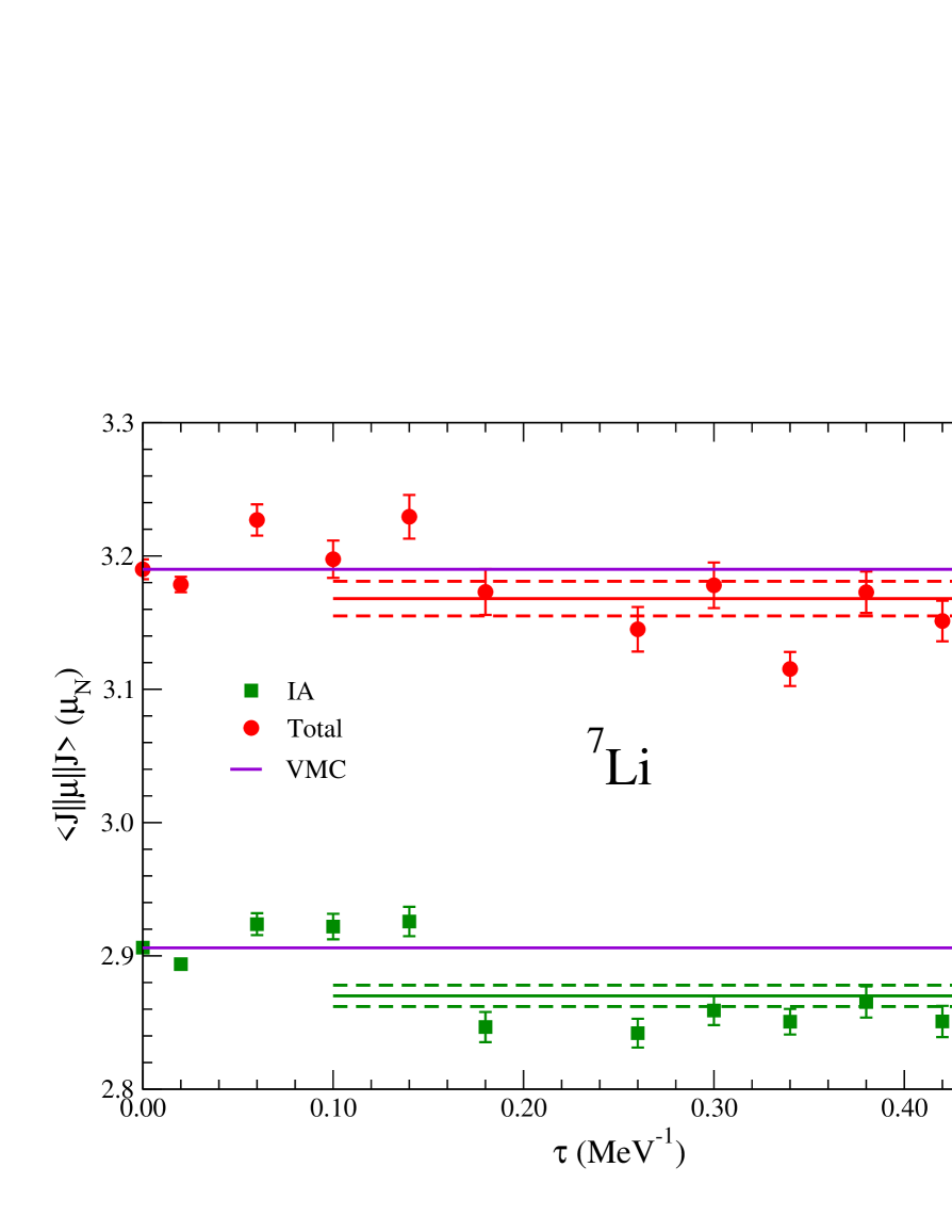
Figure 3: (Color online) Extrapolated GFMC magnetic moment for the ⁷Li$(\frac{3}{2}^{-})$ ground state in impulse approximation (green squares) and with MEC (red circles). VMC values (purple lines) and averaged GFMC values (lines with error bars) are also shown.

The GFMC propagation for the magnetic moment of the ⁷Li$(\frac{3}{2}^{-})$ ground state is shown in Fig. 3. In this figure the two solid purple lines correspond to the VMC (impulse and total) values, the green squares (red circles) are extrapolated GFMC impulse (total) propagations and the solid green (red) lines starting at $\tau$=0.1 MeV^-1 are the final GFMC averages with dashed lines to denote the Monte Carlo error. The GFMC propagation reduces the VMC matrix element slightly in both cases. The GFMC impulse result is only 88% of the experimental value, but the MEC contributions raise the total to 97%.

IV.2 Magnetic Dipole Transitions in $A$=6,7 Nuclei

In Table 4 we present the different contributions to the matrix elements for $M1$ transitions in $A$=6,7 nuclei. As in the case of magnetic moment calculations, we see that the most significant contributions come from the pseudoscalar and vector pieces of the two-body current operators.

Table 4: Matrix elements of $M1$ transitions in $A$=6,7 nuclei. Column headings are defined in Table 3.

$J^{\pi}_{i}\to J^{\pi}_{f}$	Method	IA	MEC				Total
			PS$+$V	MS	MD	$\Delta$
6Li$(0^{+};1)\to^{6}$Li$(1^{+};0)$	VMC	3.683(14)	0.307	0.003	0.010	-0.053	3.950(14)
6Li$(0^{+};1)\to^{6}$Li$(1^{+};0)$	GFMC	3.587(16)	0.323	0.002	0.012	-0.048	3.876(14)
7Li$(\frac{1}{2}^{-})\to^{7}$Li$(\frac{3}{2}^{-})$	VMC	2.743(17)	0.396	0.006	-0.017	-0.034	3.162(22)
7Li$(\frac{1}{2}^{-})\to^{7}$Li$(\frac{3}{2}^{-})$	GFMC	2.677(19)	0.395	0.011	-0.017	0.072	3.138(22)
7Be$(\frac{1}{2}^{-})\to^{7}$Be$(\frac{3}{2}^{-})$	VMC	2.420(30)	0.390	-0.005	0.010	-0.024	2.791(36)
7Be$(\frac{1}{2}^{-})\to^{7}$Be$(\frac{3}{2}^{-})$	GFMC	2.374(31)	0.394	-0.010	0.010	-0.002	2.766(36)

The first two rows of Table 4 show the various pieces of the $M1$ matrix element for ⁶Li$(0^{+};1)\to^{6}$Li$(1^{+};0)$ transition. We note that both VMC and GFMC IA results are boosted by 7–8% by MEC. The corresponding decay widths for this transition are presented in Table 5. The total width we obtain from the VMC calculation agrees very well with the experimental value, whereas the total GFMC width is slightly outside of the present experimental range. Figure 4 shows the matrix elements for this case as a function of $\tau$. As in the previous figure, the two solid purple lines represent the VMC impulse and total estimates, the green squares represent the GFMC propagated points for impulse and the red circles denote the total GFMC matrix elements. The average GFMC results are shown as solid lines with error bars starting at $\tau$=0.1 MeV^-1. All the GFMC points as well as the averages represent the extrapolated matrix elements. We note that, also in the present case, the GFMC propagation slightly decreases the VMC value for the ⁶Li$(0^{+};1)\to^{6}$Li$(1^{+};0)$ transition. We see that the propagated points are quite stable with $\tau$, which we ran up to $0.3$ MeV^-1 in this case.

Table 5: Impulse approximation (IA) and total $M1$ transition widths in eV for $A$=6,7 nuclei.

$J^{\pi}_{i}\to J^{\pi}_{f}$	Mode	VMC		GFMC		Expt.
		IA	Total	IA	Total
6Li$(0^{+};1)\to^{6}$Li$(1^{+};0)$	$M1$	7.09(6)	8.15(6)	6.72(6)	7.85(6)	8.19(17)
7Li$(\frac{1}{2}^{-})\to^{7}$Li$(\frac{3}{2}^{-})$	$M1$ ($10^{-3}$)	4.75(6)	6.31(9)	4.52(6)	6.21(9)	6.30(31)
7Be$(\frac{1}{2}^{-})\to^{7}$Be$(\frac{3}{2}^{-})$	$M1$ ($10^{-3}$)	2.62(7)	3.49(9)	2.52(7)	3.42(9)	3.43(45)

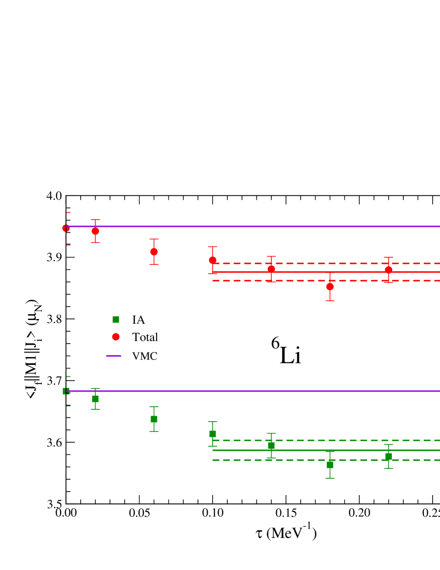
Figure 4: (Color online) Extrapolated GFMC $M1$ matrix element for the ⁶Li$(0^{+};1)\to^{6}$Li$(1^{+};0)$ transition in impulse approximation (green squares) and with MEC (red circles). VMC values (purple lines) and averaged GFMC values (lines with error bars) are also shown.

Table 5 also shows two $M1$ transitions in $A$=7 nuclei. The MEC corrections are 15–17$\%$ of the $M1$ matrix elements obtained in both VMC and GFMC calculations. The model independent pieces (PS+V) are the largest contributions and are also very similar for both ⁷Li and ⁷Be. The decay widths for ⁷Li$(\frac{1}{2}^{-})\to^{7}$Li$(\frac{3}{2}^{-})$ and ⁷Be$(\frac{1}{2}^{-})\to^{7}$Be$(\frac{3}{2}^{-})$ $M1$ transitions are shown in Table 5. The total widths from both VMC and GFMC match very well with the experimental decay widths.

V Conclusions

In summary, we have reported results for the magnetic moments and magnetic dipole transitions in nuclei with mass numbers $A\leq 7$. The calculations have used essentially exact wave functions derived from a realistic Hamiltonian that reproduces well the low-lying spectra of these nuclei as well as of those in the mass range $A$=8–10. Leading terms in the nuclear electromagnetic current have been constructed to satisfy current conservation with the two-nucleon potential, AV18, used in the Hamiltonian. Additional contributions associated with the explicit presence of $\Delta$ isobar degrees of freedom have been accounted for by including, in an approximate fashion, $\Delta$ components in the nuclear wave functions with the transition-correlation-operator method.

Overall, the agreement between the calculated and experimental magnetic moments and transition rates is quite satisfactory, particularly in the isovector channel where differences between computed and experimental amplitudes are $\simeq 1.5$%. On the other hand, in the isoscalar channel these differences seem to progressively become worse as the mass number increases; they are about 1% in deuteron, 4% in ³He/³H, and 10% in ⁷Be/⁷Li. Of course, isoscalar transitions are suppressed both at the one- and two-body levels: the IA current is proportional to the nucleon isoscalar magnetic moment, which is five times smaller than the corresponding isovector combination; leading two-body currents from pion-exchange and $\Delta$ excitation have isovector character. Two-body isoscalar contributions arise in the present study from short-range mechanisms: the momentum-dependent components of the AV18, the $\rho\pi\gamma$ transition current, and renormalization corrections induced by $\Delta$ admixtures in the wave functions, Eq. (59).

We conclude by noting that in a chiral effective-field-theory framework isoscalar corrections are suppressed by $(Q/\Lambda_{\chi})^{2}$ ($Q$ denotes a generic small momentum and $\Lambda_{\chi}\simeq 1$ GeV is the chiral-symmetry-breaking scale) relative to the leading-order (LO) IA current Pastore08a ; Pastore08b . These N²LO corrections have been calculated in the deuteron and trinucleon isoscalar magnetic moments, and are $\simeq 1$% relative to LO but of opposite sign, so that they increase the discrepancy between theory and experiment. At N³LO, or $(Q/\Lambda_{\chi})^{3}$, a number of isoscalar two-body currents originate from four-nucleon contact interactions involving two gradients of the nucleon fields Pastore08b . Their contributions to electromagnetic observables have yet to be calculated. It will be interesting to see whether these isoscalar currents as well as the corresponding isovector ones up to N³LO will improve the present picture.

- (1) M. Pervin, S. C. Pieper, and R. B. Wiringa, Phys. Rev. C 76, 064319 (2007).
- (2) R. B. Wiringa, V. G. J. Stoks, and R. Schiavilla, Phys. Rev. C 51, 38 (1995).
- (3) S. C. Pieper, V. R. Pandharipande, R. B. Wiringa, and J. Carlson, Phys. Rev. C 64, 014001 (2001).
- (4) S. C. Pieper and R. B. Wiringa, Annu. Rev. Nucl. Part. Sci. 51, 53 (2001).
- (5) S. C. Pieper, K. Varga, and R. B. Wiringa, Phys. Rev. C 66, 044310 (2002).
- (6) S. C. Pieper, R. B. Wiringa, and J. Carlson, Phys. Rev. C 70, 054325 (2004).
- (7) S. C. Pieper, Nucl. Phys. A751, 516c (2005).
- (8) J. Carlson and R. Schiavilla, Rev. Mod. Phys. 70, 743 (1998).
- (9) R. B. Wiringa and R. Schiavilla, Phys. Rev. Lett. 81, 4317 (1998).
- (10) R. B. Wiringa, Phys. Rev. C 43, 1585 (1991).
- (11) B. S. Pudliner, V. R. Pandharipande, J. Carlson, S. C. Pieper, and R. B. Wiringa, Phys. Rev. C 56, 1720 (1997).
- (12) N. Metropolis, A. W. Rosenbluth, M. N. Rosenbluth, A. H. Teller, and E. Teller, J. Chem. Phys. 21, 1087 (1953).
- (13) J. Carlson, Phys. Rev. C 36, 2026 (1987).
- (14) J. Carlson, Phys. Rev. C 38, 1879 (1988).
- (15) R. B. Wiringa, S. C. Pieper, J. Carlson, and V. R. Pandharipande, Phys. Rev. C 62, 014001 (2000).
- (16) L. E. Marcucci, M. Viviani, R. Schiavilla, A. Kievsky, and S. Rosati, Phys. Rev. C 72, 014001 (2005).
- (17) D. O. Riska, Phys. Rep. 181, 207 (1989).
- (18) D. O. Riska, Phys. Scr. 31, 107 (1985).
- (19) R.G. Sachs, Phys. Rev. 74, 433 (1948).
- (20) L. E. Marcucci, D. O. Riska, and R. Schiavilla, Phys. Rev. C 58, 3069 (1998).
- (21) J. Carlson, D. O. Riska, R. Schiavilla, and R. B. Wiringa, Phys. Rev. C 42, 830 (1990).
- (22) R. Schiavilla and D. O. Riska, Phys. Rev. C 43, 437 (1991).
- (23) M. Viviani, R. Schiavilla, and A. Kievsky, Phys. Rev. C 54, 534 (1996).
- (24) M. Viviani, A. Kievsky, L. E. Marcucci, S. Rosati, and R. Schiavilla, Phys. Rev. C 61, 064001 (2000).
- (25) D. Berg et al., Phys. Rev. Lett. 44, 706 (1980).
- (26) M. Chemtob and M. Rho, Nucl. Phys. A163, 1 (1971).
- (27) R. B. Wiringa, R. A. Smith, and T. L. Ainsworth, Phys. Rev. C 29, 1207 (1984).
- (28) R. Schiavilla, R. B. Wiringa, V. R. Pandharipande, and J. Carlson, Phys. Rev. C 45, 2628 (1992).
- (29) C. E. Carlson, Phys. Rev. D 34, 2704 (1986).
- (30) D. Lin and M. K. Liou, Phys. Rev. C 43, R930 (1991).
- (31) T. E. O. Ericson and W. Weise, Pions and Nuclei (Clarendon Press, Oxford, 1988).
- (32) D. R. Tilley, C. M. Cheves, J. L. Godwin, G. M. Hale, H. M. Hofmann, J. H. Kelley, C. G. Sheu, and H. R. Weller, Nucl. Phys. A708, 3 (2002).
- (33) W. Nörtershäuser et al., arXiv:0809.2607.
- (34) B. S. Pudliner, V. R. Pandharipande, J. Carlson, and R. B. Wiringa, Phys. Rev. Lett. 74, 4396 (1995).
- (35) J. L. Forest, V. R. Pandharipande, S. C. Pieper, R. B. Wiringa, R. Schiavilla, and A. Arriaga, Phys. Rev. C 54, 646 (1996).
- (36) S. Pastore, R. Schiavilla, and J.L. Goity, proceedings of the Fourth Asia-Pacific Conference on Few-Body Problems in Physics, Depok, Indonesia, August 19–23, 2008, to be published in Mod. Phys. Lett. A; arXiv:0809.2555.
- (37) S. Pastore, R. Schiavilla, and J.L. Goity, in preparation.