\authorinfo

Further author information: (Send correspondence to M. E. F.)
M. E. F.: E-mail: mfilho@astro.up.pt, Telephone: +351 6089 853

Phase Referencing in Optical Interferometry

Mercedes E. Filho\supita Paulo Garcia\supita,b Gilles Duvert\supitc Gaspard Duchene\supitd Eric Thiebaut\supite John Young\supitf Olivier Absil\supitg Jean-Phillipe Berger\supitg Thomas Beckert\supith Sebastian Hoenig\supith Dieter Schertl\supith Gerd Weigelt\supith Leonardo Testi\supiti Eric Tatuli\supiti Virginie Borkowski\supitj Michaël de Becker\supitj Jean Surdej\supitj Bernard Aringer\supitk Joseph Hron\supitk Thomas Lebzelter\supitk Andrea Chiavassa\supitl Romano Corradi\supitl Tim Harries\supitm \skiplinehalf\supitaCentro de Astrofisica da Universidade do Porto Rua das Estrelas 4150-762 Porto Portugal
\supitb Departamento de Engenharia Física Faculdade de Engenharia Universidade do Porto Portugal
\supitcLaboratoire d’Astrophysique de Grenoble Observatoire de Grenoble BP 53 38041 Grenoble Cedex 9 France
\supitdUC Berkeley Astronomy Department 601 Campbell Hall Berkeley CA 94720-3411 USA
\supiteObservatoire de Lyon 9 Av. Charles André 69561 Saint Genis Laval Cedex France
\supitfCavendish Laboratory Madingley Road Cambridge CB3 OHE UK
\supitgUniversité J. Fourier CNRS Laboratoire d’Astrophysique de Grenoble UMR 5571 France;
\supithMax-Planck Institute for Radioastronomy Bonn Germany;
\supitiINAF/Osservatorio di Astrofisica di Arcetri Italy;
\supitjInstitute of Astrophysics and Geophysics Liège Belgium;
\supitkInstitute of Astrophysics of the University of Wien Austria;
\supitlGroupe de Recherche en Astronomie et Astrophysique du Languedoc Montpellier France;
\supitmSchool of Physics University of Exeter UK;

Abstract

One of the aims of next generation optical interferometric instrumentation is to be able to make use of information contained in the visibility phase to construct high dynamic range images.

Radio and optical interferometry are at the two extremes of phase corruption by the atmosphere. While in radio it is possible to obtain calibrated phases for the science objects, in the optical this is currently not possible. Instead, optical interferometry has relied on closure phase techniques to produce images. Such techniques allow only to achieve modest dynamic ranges. However, with high contrast objects, for faint targets or when structure detail is needed, phase referencing techniques as used in radio interferometry, should theoretically achieve higher dynamic ranges for the same number of telescopes.

Our approach is not to provide evidence either for or against the hypothesis that phase referenced imaging gives better dynamic range than closure phase imaging. Instead we wish to explore the potential of this technique for future optical interferometry and also because image reconstruction in the optical using phase referencing techniques has only been performed with limited success.

We have generated simulated, noisy, complex visibility data, analogous to the signal produced in radio interferometers, using the VLTI as a template. We proceeded with image reconstruction using the radio image reconstruction algorithms contained in aips imagr (clean algorithm). Our results show that image reconstruction is successful in most of our science cases, yielding images with a 4 milliarcsecond resolution in K band.

We have also investigated the number of target candidates for optical phase referencing. Using the 2MASS point source catalog, we show that there are several hundred objects with phase reference sources less than 30 arcseconds away, allowing to apply this technique.

keywords:

optical interferometry

1 INTRODUCTION

An ideal interferometer will measure the complex visibility of an astronomical object. Image reconstruction deals with inverting the visibility information into an image, given poor Fourier plane sampling and limited phase information.

In an array of N telescopes, signals are combined in $\frac{1}{2}$ $\times$ N $\times$ (N-1) pairs or baselines to obtain $\frac{1}{2}$ $\times$ N $\times$ (N-1) measurements called complex visibilities. These visibilities are related to the object brightness distribution via the van Cittert-Zernike theorem:

$V(u,v)=\int\int I(x,y)\,exp[-2\,\pi\,i\,(ux+vy)]dx\,dy$

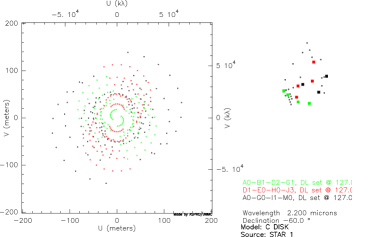
where x and y are angular displacements on the plane of the sky with the phase center as origin, I(x,y) is the brightness distribution of the target and u and v are the position vectors of the baselines projected on a plane perpendicular to the source direction, which together define the uv plane. In practical terms, the better the sampling of the uv plane in terms of baseline length, position angle, and number of measurements, the more faithful the reconstructed image will be relative to the true brightness distribution.

Radio-type observations are performed by measuring the amplitudes (modulus) and the phases (argument) of the complex visibilities:

$V(u,v)=A\,exp(i\,\phi)$

Image reconstruction using the modulus and argument of the visibility function is called phase referencing image reconstruction and is widely used in radio astronomy. Studies of this type were previously attempted by Masoni (2006), Masoni et al. (2005) and Weigelt et al. (2008; private communication).

2 Array Configuration

Telescope configurations are an essential part of the image reconstruction process. We began by identifying array configurations that allowed the most uniform uv coverage:

Refer to caption — Figure 1: 4 UT $\times$ 1 night configuration.

•

4 UTs $\times$ 1 night –- the chosen configuration when observing very faint sources (Fig. 1);
•

4 ATs $\times$ 3 nights –- the case where there is a small number of telescopes (Fig. 2);
•

6 ATs $\times$ 1 night –- a 6 telescope extended configuration with one night observation; has less $uv$ points than the 4 AT x 3 nights configuration but comparable $uv$ coverage (Fig. 3).

3 Noise Model

The noise model estimates the uncertainties on the visibility amplitudes and phases assuming an instrument following a multi-axial recombination scheme with a fringe tracker (FT; Jocou et al. 2007).

The quantity we procure is the total number of detected photoevents per integration time per pixel per baseline in the interferometric channel:

${\overline{N}_{i}}=\frac{N_{total}*f}{N_{pix}*N_{base}}$

where $f$ is the fraction of the beam that gores into the interferometric channel (90%), $N_{pix}$ is the number of pixels needed to read the interferometric channel (600), $N_{base}$ is the number of baselines and $N_{total}$ is the total number of detected photevents per integration time per pixel in all channels:

$N_{total}=F_{0}*10^{-0.4mag}*t_{int}*N_{tel}*\pi*R^{2}*\Delta\lambda*trans*Strehl$

Here $F_{0}$ is the photon flux of a zeroth magnitude star (Jocou et al. 2007), $mag$ is the object magnitude in the observing band, $t_{int}$ is the integration time, $N_{tel}$ is the number of telescopes (6 or 4), $R$ is the radius of the telescopes (4.1 for UTs and 0.9 for ATs) assumed for simplification to have no central hole, $\Delta\lambda$ is the spectral bandwidth (chosen), $trans$ is the total instrument transmission including quantum efficiency (Jocou et al. 2007), and $Strehl$ is the Strehl ratio and depends on wavelength (Jocou et al. 2007).

Therefore, the total number of detected photevents in the interferometric channel is:

$N_{i}={\overline{N}_{i}}*N_{pix}*N_{int}$

where $N_{int}$ is the number of independent integrations (depends on magnitude and FT presence).

The object intrinsic visibility, $V$ , must be corrected for the instrumental visibility loss (80%) and the instrumental visibility loss induced by the FT (90%). The correlated flux per baseline is therefore:

$F_{cor}=N_{i}*\frac{V^{\prime}}{2}$

and finally the error in visibility is given by:

$error_{V}=\sqrt{F_{cor}+N_{int}*N_{pix}*\sigma^{2}}$

where $\sigma$ os the readout noise of the detector (15 e-).

4 UVFITS File Generation

UVFITS is the file format in which radio astronomical data are written and used for phase referencing image reconstruction. UVFITS format is designed so that different categories of information are stored in distinct “tables” within a file and can be cross-referenced one to another. Each UVFITS file “table” stores specific parameters that include important interferometric observables and system information.

Key science images were generated and provided by the science case groups (Garcia et al. 2007). Using aspro, an image simulation tool originally created for IRAM, and the configurations above, K band ”images” of the sources were created assuming that all sources were observed at the fixed declination of $-$ 60 degrees.

It was assumed also that during the night, the telescope configurations would remain fixed and that one calibrated uv point per baseline should be obtained every hour. The actual on-source integration time is, however, 10-15 minutes per hour due to overheads. The total integration time assumes an entire transit (9 hours).

5 Phase Referencing Theory

A radio interferometer works by phase referencing. The interferometer observes a science target and records the visibility modulus and phase for each baseline. It also observes a reference target used to calibrate the visibility modulus and phase for atmospheric variations. Therefore, as opposed to conventional optical interferometry, phase referencing makes use of crucial information contained in the phases to recover the brightness distribution of a source.

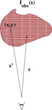Given an incoherent source, the observed brightness distribution in a direction $\vec{s^{\prime}}$ is given by:

$I^{obs}(\vec{s^{\prime}})=I^{obs}(x,y)=PSF(x,y)*I^{true}(x,y)+N(x,y)$

where PSF(x,y) is the instrumental point spread function, I^true(x,y) is the true object brightness distribution, N(x,y) is the noise and the asterisk denotes convolution.

In practice, interferometry does not make measurements in the image plane but in Fourier space. The relevant quantity is called the complex visibility and is measured at each uv point, the position vector of the baseline on a plane perpendicular to the source direction:

$V^{obs}(u,v)=S(u,v)\times V^{true}(u,v)+N^{\prime}(u,v)$

where S(u,v), the sampling function, is the Fourier transform of the PSF(x,y), V^true(x,y), the true visibility, is the Fourier transform of the true brightness distribution I^true(x,y) and N’(u,v) is the noise in the Fourier space.

The van Cittert-Zernike theorem states that the true brightness distribution can be obtained by the inverse Fourier transform and deconvolution of the observables:

$I^{true}(x,y)*PSF(x,y)=\int\int V^{true}(u,v)\times S(u,v)\,exp\,[2\pi i(ux+vy)]\,du\,dv$

The role of image reconstruction is to obtain the best approximation, I^aprox(x,y) $\sim$ I^obs(x,y) $\sim$ I^true(x,y), to the true brightness distribution.

In radio-like phase referencing image reconstruction, the data are gridded, interpolated and inverse Fourier transformed to yield a model representation of the sky:

$I^{dirty}(x,y)=I^{aprox}(x,y)*PSF^{dirty}(x,y)+N(x,y)$

where $I^{dirty}(x,y)$ is called the dirty map and $PSF^{dirty}(x,y)$ is called the dirty beam.

The NRAO Astronomical Image Processing System (aips), is a baseline-based reconstruction method used in radio interferometry. The UVFILES generated by aspro were imported into aips. We have tested the results using the clean algorithm (Högbom 1974), which corrects for the effect of poor Fourier plane sampling. clean grids, Fourier transforms and deconvolves the dirty beam from the dirty image in an iterative fashion given an initial guess for the beam and the brightness distribution. clean then finds peaks in the residual image and subtracts $\delta$ functions of the appropriate strength at those positions. The final map is a convolution of all the $\delta$ functions with a clean beam plus the residual map.

6 Image Analysis

In order to compare the reconstructed with the synthetic images, aspro was used to generate the point spread functions (PSF) for the 6 AT $\times$ 1 night, 4 AT $\times$ 3 nights and 4 UT $\times$ 1 night configurations (Table 1). The synthetic images were then convolved with a Gaussian of the measured PSF parameters (iraf program gauss).

Table 1: PSF parameters. Col. 1: Configuration. Col. 2: Full width at half maximum. Col. 3: Dispersion,

\sigma=FWHM/2.35

. Col. 4: Elllipticity,

e=\frac{a-b}{a+b}

, where

a

is the major and

b

the minor axis. Col. 5: Axis ratio,

r=\frac{1-e}{1+e}

. Col. 6: Position angle of the minor axis.

Configuration	FWHM	$\sigma$	e	r	PA
4 UT $\times$ 1 night	4.45	1.89	0.08	0.85	$-$ 9.0^⋅
4 AT $\times$ 3 nights	3.51	1.49	0.38	0.45	$-$ 83.0^⋅
6 AT $\times$ 1 night	5.17	2.20	0.42	0.41	$-$ 85.0^⋅

Relative astrometry information was obtained for the images using ds9. Photometry of the image components was performed using iraf procedure phot. $SNR$ is the ratio of the mean pixel value to the standard deviation meansured on the reconstructed images.

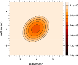
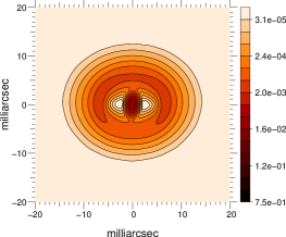
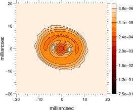
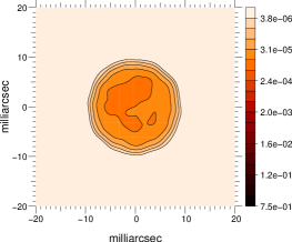
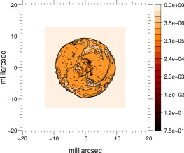
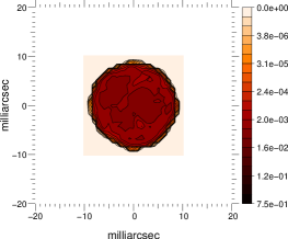
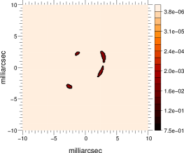
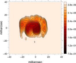
7 Phase Referencing Image Reconstruction

Table 2: AGN. Diameter units are pixels.

	Image 4 UT	aips 4 UT
flux sublimation	84.9%	97.0%
flux torus	15.1%	3.0%
ratio	5.6	32.3
sublimation diameter	50	45
torus diameter	260	-
SNR	-	89

Table 3: Evolved Star. Diameter units are pixels.

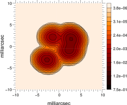
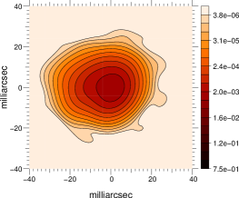
	Image 4 AT 3	aips 4 AT 3	Image 6 AT	aips 6 AT
flux star	21.9%	29.4%	21.9%	28.7%
flux wind	78.1%	70.6%	78.1%	71.3%
ratio star/wind	0.3	0.4	0.3	0.4
inner wind diameter	50 $\times$ 35	50 $\times$ 35	50 $\times$ 35	50 $\times$ 35
outer wind diameter	100 $\times$ 85	100 $\times$ 85	100 $\times$ 85	100 $\times$ 85
SNR	-	46	-	23

Table 4: Microlensing. Distance units are pixels.

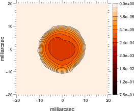
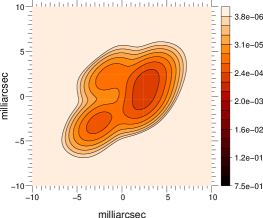
	Image 4 UT	aips 4 UT
A flux	12.8%	12.9%
B flux	19.2%	19.6%
C flux	68.0%	67.5%
ratio C/A	5.3	5.2
ratio C/B	3.5	3.4
distance AC	45	45
distance BC	70	70
distance AB	50	50
SNR	-	99

Table 5: Pinwheel

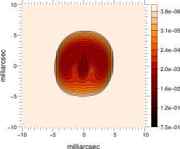
	Angle	Image 6 AT	aips 6 AT	SNR
inner spiral	0 deg	24 $\times$ 30	24 $\times$ 24	281
inner spiral	60 deg	24 $\times$ 24	24 $\times$ 22	404

Table 6: YSO. Diameter units are pixels.

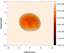
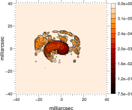
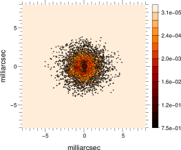
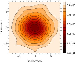
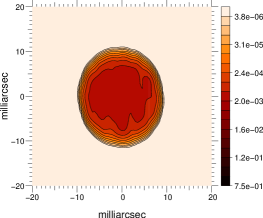
	Image 4 UT	aips 4 UT	Image 4 AT 3	aips 4 AT 3	Image 6 AT	aips 6 AT
flux star	15.7%	-	18.1%	-	18.1%	16.7%
flux disk	84.3%	-	81.9%	-	81.9%	83.3%
ratio	0.2	-	0.2	-	0.2	0.2
outer diameter	60 $\times$ 40	60 $\times$ 40	70 $\times$ 60	70 $\times$ 60	80 $\times$ 70	80 $\times$ 70
SNR	-	1	-	184	-	530

8 Discussion

If we compare the reconstructed images with the convolved images, we see that the phase referencing image reconstruction has yielded good results. Most of the flux is recovered in the individual image elements and the astrometry is excellent. A clear example of this is the reconstructed stellar surface images. Most of the flux is recovered in a compact region and careful inspection of the reconstructed images shows correspondence with individual brightness regions in the convolved image. The edges of the stellar surface are also well reproduced.

For an array of $N$ telescopes, the total number of measurements per observing night per integration point (moduli plus phase over each baseline) in phase referencing is $N\times(N-1)$ compared to $\frac{(N-1)}{2}\times(\frac{3}{2}N-2)$ closure phases plus squared visibilities in conventional phase closure techniques. As an example, when $N=4$ , there are 6 measured parameters for phase closure observations and 12 for phase referencing. Therefore, phase referenced reconstructed images should theoretically be more rigorous.

9 Observable Objects

In order to perform real time phase referencing observations, it is necessary to have a phase reference source no more than 30” away from the target source. For larger distances, the atmospheric pistons become distinct and the calibration incorrect.

Among the science cases presented, the most crucial in terms of number of phase reference candidates are the AGN, due to their large distances and therefore their K band faintness. We have attempted to quantify the number of AGN for which phase reference imaging is possible by using the Véron-Cetty & Véron (2006) catalog which contains AGNs, QSOs and BL Lac objects. Firstly, we constrained the science targets to those visible to the VLTI: targets were chosen to be between $+$ 20 and $-$ 90 degree declination. We then searched the 2MASS point source catalog for a nearby (less than 30” from the science target) bright star suitable for both AO wavefront sensing and fringe tracking (i.e., star mangitudes $K<$ 10, $R<$ 16). Science targets are listed in Table 7.

Table 7: Science target list of all southern (declination +20 to -90^∘) AGNs in the Véron-Cetty & Véron catalog (2006) with a bright star (

K<10

and

R<16

) in their isoplanatic patch (i.e., star separation

<

30 arcsec). These nearby stars are suitable for both AO wavefront sensing and fringe tracking. The

K_{core}

magnitudes are the

K

magnitudes from the 2mass catalog, the

K_{star}

and

R_{star}

magnitudes are the magnitudes of the nearby stars.

Name	type	RA	DEC	$K_{core}$	$K_{star}$	$R_{star}$
J004336.0+001456	Sy1	00 43 36.0	+00 14 56	14.6	9.4	10.7
LEDA101303	LIN	01 38 52.9	-10 27 11	13.6	8.5	10.7
NGC 676	Sy2	01 48 57.3	+05 54 24	11.1	8.6	10.1
J024613.8+105656	QSO	02 46 13.8	+10 56 56	13.7	9.0	10.9
NGC1204	Sy2	03 04 40.0	-12 20 29	11.4	9.1	10.0
HE 0324-3652	QSO	03 26 01.0	-36 41 49	13.9	9.7	12.8
LEDA13424	LIN	03 38 40.5	+09 58 12	12.4	8.1	12.6
ESO548-81	Sy1	03 42 03.6	-21 14 37	10.5	6.0	8.4
LEDA 2824014	QSO	04 37 36.6	-29 54 02	14.3	7.0	8.0
LEDA2824155	Sy1	04 56 08.9	-21 59 09	13.4	9.6	11.0
4U0517+17	Sy1	05 10 45.5	+16 29 57	11.6	6.2	9.2
J052223.1-072513	Sy1	05 22 23.1	-07 25 13	13.0	9.5	10.5
J062233.8-231743	Sy1	06 22 33.4	-23 17 42	13.0	9.4	11.3
J063635.8-622032	LIN	06 36 35.8	-62 20 32	14.2	8.4	10.0
J083750.7+091218	Sy1	08 37 50.7	+09 12 18	14.9	8.8	10.5
2E2060	Sy1	08 52 15.1	+07 53 37	12.6	9.2	10.8
J091034.3+031328	AGN	09 10 34.3	+03 13 28	14.0	9.7	11.3
J091430.4+104906	Sy1	09 14 30.4	+10 49 06	14.7	9.3	10.5
J095916.7-073517	Sy1	09 59 16.7	-07 35 17	13.1	9.2	11.1
LEDA31718	Sy1	10 39 46.3	-05 28 59	12.8	9.2	11.3
RBS 999	Sy1	11 34 22.5	+04 11 28	12.9	8.8	10.5
MGC 24800	AGN	11 48 16.0	-00 03 29	14.0	8.4	11.3
J120001.9+023418	Sy2	12 00 01.9	+02 34 18	14.5	9.1	11.2
J120848.9+101343	AGN	12 08 48.9	+10 13 43	14.3	9.8	11.0
J121855.8+020002	QSO	12 18 55.8	+02 00 02	14.8	9.6	11.1
J130335.3-004912	Sy1	13 03 35.3	-00 49 12	14.7	9.2	11.5
HE 1304-0541	QSO	13 06 47.6	-05 57 35	14.7	8.1	10.2
J130838.2-825934	QSO	13 08 38.2	-82 59 34	14.6	8.7	11.4
J132301.0+043951	BLL	13 23 01.0	+04 39 51	14.4	9.7	10.9
LEDA 170317	Sy2	13 58 59.7	-20 02 43	12.3	8.2	8.0
J152929.3+033137	Sy2	15 29 29.3	+03 31 37	14.7	9.1	11.2
MCG+03-40-009	Sy2	15 35 52.6	+14 31 04	12.9	9.6	12.5
J154025.1+030640	Sy2	15 40 25.1	+03 06 40	15.0	9.4	11.3
ESO 137-34	Sy2	16 35 14.2	-58 04 41	11.4	7.3	9.2
LEDA 2829294	QSO	17 33 02.6	-13 04 50	14.2	7.4	14.8
J173728.3-290802	Sy1	17 37 28.3	-29 08 02	11.1	8.7	11.0
IGR J18027-1455	Sy1	18 02 47.3	-14 54 54	10.9	8.6	15.2
LEDA 86291	Sy1	18 51 59.5	+11 52 33	11.0	9.9	14.2
J193109.5+093713	BLL	19 31 09.8	+09 37 04	14.4	8.9	13.5
LEDA 65714	Sy1	20 55 22.3	+02 21 17	12.5	9.6	12.7
1H 2107-097	Sy1	21 09 09.9	-09 40 15	10.9	8.8	12.1
J211837.3-010537	AGN	21 18 37.3	-01 05 37	8.14	8.1	12.3
J220555.0-000755	Sy2	22 05 55.0	-00 07 55	14.8	8.9	11.6
J223013.4-292554	QSO	22 30 13.4	-29 25 54	14.9	9.8	11.0
MCG+01-57-007	Sy1	22 32 30.8	+08 12 27	11.8	9.3	10.7

We have also investigated the number of phase reference targets available from a series of stellar catalogs. No trimming of objects for observability (southern hemisphere or target magnitude) was done. The following catalogs were searched: the de Winter et al. (2001) catalog of southern emission line objects mainly containing Herbig Ae/Be stars and some B[e], LBV and TTauri stars; the Egret (1980) catalog of supergiants; the Fracassini et al. (1994) catalog of stellar radii trimmed to objects with diameters of at least 10 mas; the Ramos-Larios & Phillips (2005) catalog of planetary nebulae; the Herbig & Bell (1995) catalog of pre-main-sequence stars; the Muench et al. (2002) catalog of pre-main-sequence stars in the Orion Trapezium cluster. We have searched for appropriate phase reference 2MASS point sources with K band magnitudes between 9 and 11 less then 30” away from the targets. The results are presented in Table 8 and highlight the potencial of phase reference imaging.

Table 8: Science target list with a bright star (9

<

<

11) in their isoplanatic patch (i.e., star separation

<

30 arcsec). These nearby stars are suitable for fringe tracking.

Catalog	Science	Total Number of Targets	Total Number of Targets
Reference	Targets	in the Catalog	with Phase Ref. Sources
de Winter et al.	Herbig Ae/Be, LBV & T Tauri	162	62
Egret	supergiants	5073	1253
Fracassini et al.	stars with d $<$ 10 mas	143	8
Ramos-Larios & Phillips	planetary nebulae	325	68
Herbig & Bell	pre-main sequence stars	763	217
Muench et al.	pre-main sequence stars
	in the Orion Trapezium cluster	1 010	875
Véron-Cetty & Véron	AGN, BL Lacs & QSOs	108 080	133

10 Conclusions

Theoretically it is found that phase reference image reconstruction should yield more rigourous images than the classical phase closure method used in optical interferometry, not only because longer integrations times are allowed, but also because the former method measures information related to the visibility phase.

We wished to explore the potential of phase referencing in optical interferometry. We have generated simulated, noise visbility amplitudes and phases using the VLTI as a template and reconstructed images with the classic radio interferometry algorithm clean contained in the aips package. Our results show that with this method we will be able to reconstruct images of diverse sources with a spatial resolution of about 4 milliarcseconds in K band.

We have also compiled a list of target sources for which optical phase referencing is possible and found several hundred candidates.

11 Acknowledgments

We would like to thank J. Brinchmann for his help with the phase reference sources. MEF is supported by the Funda cão para a Ciência e a Tecnologia through the research grant SFRH/BPD/36141/2007. PJVG and MEF were supported in part by the Funda cão para a Ciência e a Tecnologia through projects PTDC/CTE-AST/68915/2006 and PTDC/CTE-AST/65971/2006 from POCI, with funds from the European programme FEDER.

12 References

Egret, D. 1980, Bulletin d’Information du Centre de Donnees Stellaires, 18, 82

Fracassini, M., Pasinetti-Fracassini, L. E., Pastori, L., & Pironi, R. 1994, VizieR Online Data Catalog, 2155, 0

Garcia, P. et al. 2007, in doc. VLT-SPE-VSI-15870-4335, issue 1.0 in VSI Phase A Document Package, Science Cases

Herbig, G. H., & Bell, K. R. 1995, VizieR Online Data Catalog, 5073, 0

Högbom, J. A., 1974, A&AS, 15, 417

Jocou, L. et al. 2007, in doc. VLT-SPE-VSI-15870-4335, issue 1.0 in VSI Phase A Document Package, System Design

Masoni, L. 2006, PADEU, 17, 155

Masoni, L. et al. 2005, Astr. Nachr., 326, 566

Muench, A. A., Lada, E. A., Lada, C. J., & Alves, J. 2002, ApJ, 573, 366

Ramos-Larios, G., & Phillips, J. P. 2005, MNRAS, 357, 732

Véron-Cetty, M. -P. & Véron, P. 2006, A&A, 455, 773

de Winter, D., van den Ancker, M. E., Maira, A., Thé, P. S., Djie, H. R. E. T. A., Redondo, I., Eiroa, C., & Molster, F. J. 2001, A&A, 380, 609