Semileptonic decays in the limit of a heavy daughter quark

Abstract

The rate of the semileptonic decay $b\to c\ell\nu$ is calculated with $\mathcal{O}\left(\alpha_{s}^{2}\right)$ accuracy, as an expansion around the limit of equal masses of the $b$ and $c$ quarks. Recent results obtained around the limit of the $c$-quark much lighter than $b$ are confirmed. Details of the new expansion method are described.

I Introduction

Very recently, next-to-next-to-leading order (NNLO) QCD corrections to the semileptonic $b\to c$ decay were calculated with full account of the charm quark mass Melnikov:2008qs ; Pak:2008qt (see also Ref. Pak:2008cp ). The former paper employed a numerical method while in the latter the decay rate was expanded in the ratio of quark masses, $\rho=m_{c}/m_{b}$. These two approaches are complementary, with the numerical one having better accuracy for the larger daughter quark mass and the analytical expansion being obviously better for a lighter one. The physically most interesting is the region of the actual quark mass ratio, $\rho\sim 0.25..0.3$. Both methods are applicable in this domain and agree very well with each other. The resulting prediction for the $b$-quark decay rate will improve the accuracy of the quark mixing parameter $V_{cb}$.

In the present paper we provide an additional check of that QCD correction. We construct an analytical expansion like in Pak:2008qt , but around the opposite limit: instead of starting with $\rho=0$ (massless charm) we expand around $\rho=1$ (equally heavy $b$ and $c$ quarks). We find that this leads to a faster convergent series whose sum smoothly matches that found in Pak:2008qt . As a result we now have a set of analytical expressions valid in the whole range of possible quark masses. In addition, the method of asymptotic expansions is applied to a new kinematic configuration.

II Calculational Method for the Decay Rate

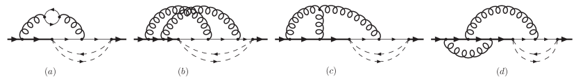
Figure 1: Sample diagrams contributing to the decay width. Thick and thin lines denote $b$ and $c$ quarks, respectively. Curly lines denote gluons and dashed lines denote leptons. All quark flavors have to be considered in the closed loop.

Using the optical theorem, we calculate the decay width from the imaginary parts of $b$-quark self-energy diagrams up to four loops, such as shown in Fig. 1. These diagrams contain two masses, $m_{b}$ and $m_{c}$, and it is not known how to compute them analytically. We thus treat the mass difference $m_{b}-m_{c}=m_{b}(1-\rho)$ as a small quantity and construct an expansion around the limit of equal masses. The expansion parameter is $\delta\equiv 1-\rho$.

This expansion is peculiar in the sense that the decay is not possible at the limiting point, $\delta=0$. This leads to a strong suppression of our result as $\rho$ tends to one and, as will be seen below, ensures good convergence of the expansion. Furthermore, there are no contributions from the region where all loop momenta are of order $m_{b}$. This makes the calculation significantly simpler than the complementary expansion around $\rho=0$ Pak:2008qt .

A somewhat similar configuration was considered in Czarnecki:2001cz , where the decay $b\to u\ell\nu$ was evaluated near the limit of the maximum invariant mass of the leptons. The difference in the present case is that it is the daughter quark that is massive and almost saturates the phase space. Since that massive quark radiates, the calculation is more involved. We explain it in some detail below.

In the first step we integrate over the loop momentum in the massless neutrino-charged lepton loop, replacing it with a fractional power of the momentum flowing through it, $1/k^{2\epsilon}$ where $D=4-2\epsilon$ is the number of dimensions in dimensional regularization. For example, Fig. 2 $(a)$ shows the lowest-order diagram; the lepton-loop momentum is $l$.

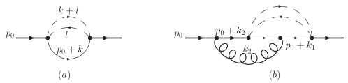
Figure 2: In $(a)$ the tree level diagram for the decay $b\to c\ell\nu$ is depicted, while $(b)$ shows the general topology of the first order correction. Thin and thick lines indicate $c$ and $b$ quarks, respectively. Dashed lines denote leptons and curly lines denote gluons.

The remaining loop momenta can have one of two characteristic scales, hard $m_{b}$ or soft $m_{b}-m_{c}=\delta\cdot m_{b}$. Depending on their configuration, the propagators can be expanded in some small parameter, leading to a factorized product of one or more single one-scale integrals Tkachov:1997gz ; Czarnecki:1996nr ; Smirnov:2002pj . This procedure is illustrated in Fig. 3 with the lowest-order example without gluons.

Full (unexpanded) diagram	$[1]=(p_{0}+k)^{2}+m_{c}^{2}$   $[2,3]=k^{2\epsilon}$
Region 1	$|k|\sim m_{b}$	$[1]\to k^{2}+2p_{0}\cdot k$
Region 2	$|k|\sim\delta m_{b}$	$[1]\to 2p_{0}\cdot k+2\delta p_{0}^{2}$

Figure 3: The asymptotic expansion of the diagram in Fig. 2 $(a)$. The dotted double line corresponds to the epsilon propagator and the double solid line corresponds to the eikonal propagator $2p_{0}\cdot k+2\delta p_{0}^{2}$

In this example, Region 1 contributes only to the real part, hence need not be considered in this calculation of the decay rate. More generally, the hard regions (when all momenta are hard, $\sim m_{b}$) will not contribute even at higher orders in $\alpha_{s}$. This removes what would otherwise be the most difficult part of the calculation. In the present expansion around $\delta=0$ there are fewer regions that need to be considered than in the expansion around $\rho=0$. At most four regions contribute to a given diagram, compared to eleven in the complementary expansion of Refs. Pak:2008qt ; Pak:2008cp . All other regions are either purely real or scaleless and give no contribution.

The second region, thus, contains full information about the tree level result. The resulting integral has already been considered in the literature Czarnecki:1997fc . Here we treat its generalization since it will be needed in the higher order corrections,

$$I(\lambda_{1},\lambda_{2},\lambda_{3}) = \int\frac{{\rm d}^{D}k}{(2\pi)^{D}}\frac{1}{(k^{2})^{\lambda_{1}}(2p_{0}\cdot k)^{\lambda_{2}}(2p_{0}\cdot k+\Delta)^{\lambda_{3}}}$$ (1)

$$= (-p_{0}^{2})^{\lambda_{1}-D/2}\Delta^{D-2\lambda_{1}-\lambda_{2}-\lambda_{3}}\frac{\Gamma(D-2\lambda_{1}-\lambda_{2})\Gamma(2\lambda_{1}+\lambda_{2}+\lambda_{3}-D)\Gamma(D/2-\lambda_{1})}{(4\pi)^{D/2}\Gamma(\lambda_{1})\Gamma(\lambda_{3})\Gamma(D-2\lambda_{1})}\,,$$ (2)

where $\Delta=2\delta p_{0}^{2}-i0$, $p_{0}^{2}=-m_{b}^{2}$, and $\lambda_{1}$, $\lambda_{2}$, and $\lambda_{3}$ are arbitrary complex numbers. In general, there would also be scalar products in the numerator, but it is well known how to deal with these Czarnecki:1997fc and bring the integral into the form of Eq. (1). This integral is one of only five general integrals needed in NLO and NNLO calculations. The other ones are on-shell propagators up to two loops and one-loop massless propagators, all of which are well known Broadhurst:1991fi .

For every topology, the most complicated integrals were encountered in the regions where all loop momenta are soft. Fortunately, these three-loop integrals could easily be written as a combination of nested integrals of the form $I(\lambda_{1},\lambda_{2},\lambda_{3})$. To illustrate this, let us consider the general two-loop integral, corresponding to Fig. 2 $(b)$ after integration of the lepton loop. If both loop momenta are soft, the integral is given by

$$\int\frac{{\rm d}^{D}k_{1}}{(2\pi)^{D}}\frac{{\rm d}^{D}k_{2}}{(2\pi)^{D}}\frac{(k_{1}\cdot k_{2})^{a_{6}}}{(k_{1}^{2})^{\epsilon+a_{1}}(2p_{0}\cdot k_{1}+\Delta)^{a_{2}}(k_{2}^{2})^{a_{3}}(2p_{0}\cdot k_{2})^{a_{4}}[2p_{0}\cdot(k_{1}+k_{2})+\Delta]^{a_{5}}}\,,$$ (3)

where the $a_{i}$ are integer numbers and $a_{6}$ is always positive. The $k_{2}$ integral can be carried out using Eq. (1) with $\Delta$ replaced by $2p_{0}\cdot k_{1}+\Delta$, performing tensor reduction in the process. The resulting $k_{1}$ integral is again of the type of Eq. (1).

For the NNLO calculation, it turned out to be useful to apply partial fraction decomposition in some cases. For example, in Eq. (3) we could also use the identity

$$\frac{1}{(2p_{0}\cdot k_{2})\,[2p_{0}\cdot(k_{1}+k_{2})+\Delta]}=\frac{1}{(2p_{0}\cdot k_{1}+\Delta)}\left(\frac{1}{2p_{0}\cdot k_{2}}-\frac{1}{2p_{0}\cdot(k_{1}+k_{2})+\Delta}\right)$$ (4)

to reduce the number of terms in the denominator. Note that the $k_{2}$ integral becomes scaleless for $a_{5}\leq 0$. While it is obviously not necessary to apply Eq. (4) in the case of the integral in Eq. (3), it was necessary to apply analogous identities in order to write some of the NNLO integrals as nested integrals of the type of Eq. (1).

New types of integrals appear only in the diagrams with three-gluon interactions (cf. Fig 1 $(c)$), due to the third gluon propagator. However, in these cases it was possible to apply the so-called Laporta algorithm Laporta:1996mq ; Laporta:2001dd to dispose of one of the three gluon propagators. The remaining integrals were again a nested set of $I$-type integrals. For this reduction we used the C++ program rows rows and the Mathematica package FIRE Smirnov:2008iw .

Our calculation was performed with two independent setups. One approach is based on the code developed for the calculation of Ref. Pak:2008qt . The other uses QGRAF Nogueira:1991ex to generate the diagrams and q2e and exp Harlander:1997zb ; Seidensticker:1999bb to process them further (no expansion is done in this step). The final calculations are in both cases done with custom code written in FORM Vermaseren:2000nd .

III Results

The result for the total width can be cast into the form

$$\Gamma = \frac{G_{F}^{2}\,|V_{cb}|^{2}\,m_{b}^{5}}{192\,\pi^{3}}\,\left[X_{0}+\frac{\alpha_{s}(m_{b})}{\pi}\,C_{F}\,X_{1}+\left(\frac{\alpha_{s}}{\pi}\right)^{2}\,C_{F}\,X_{2}+\dots\right]\,,$$ (5)

$$X_{2} = C_{F}\,X_{F}+C_{A}\,X_{A}+T_{F}\left(n_{l}\,X_{l}+X_{c}+X_{b}\right)\,,$$ (6)

where $G_{F}$ is the Fermi constant and the ellipsis denotes higher order contributions. $\alpha_{s}$ is defined with five active flavors. In QCD we have $C_{F}=4/3$, $C_{A}=3$, and $T_{F}=1/2$. $n_{l}=3$ denotes the number of light quark flavors, which are taken to be massless in our calculation. $X_{c}$ and $X_{b}$ denote the contribution from self-energy diagrams with closed $c$- and $b$-quark loops, respectively (cf. Fig 1 $(a)$). Thus, $X_{c}$ also contains contributions from real $c$-quark pairs. The quark masses are renormalized in the on-shell scheme.

The tree level and one-loop contributions can be inferred from the closed-form result of Ref. Nir:1989rm . Expanded in $\delta$ they read

$$X_{0} = \frac{64}{5}\,\delta^{5}-\frac{96}{5}\,\delta^{6}+\frac{288}{35}\,\delta^{7}+\dots\,,$$ (7)

$$X_{1} = -\frac{48}{5}\,\delta^{5}+\frac{72}{5}\,\delta^{6}+\left(-\frac{158152}{11025}+\frac{512}{105}\ln 2\delta\right)\,\delta^{7}+\dots\,,$$ (8)

where the ellipses denote higher order terms. Note that the expansion starts at the fifth power of $\delta$. Thus, the total width tends to zero very fast as $\delta$ ($\rho$) tends to zero (one). Logarithms of $\delta$ always appear as $\ln 2\delta$, since they stem solely from $\Delta$ in the integral of Eq. (1).

The first three terms in the expansion of the individual contributions read

$$X_{F} = \left[-\frac{46}{5}+\frac{32}{5}\pi^{2}\left(1-\ln 2\right)+\frac{48}{5}\zeta_{3}\right]\,\delta^{5}+\left[\frac{69}{5}-\frac{48}{5}\pi^{2}\left(1-\ln 2\right)-\frac{72}{5}\zeta_{3}\right]\,\delta^{6}$$ (9)

$$+\left(\frac{39329}{3675}+\frac{3044}{945}\pi^{2}-\frac{496}{105}\pi^{2}\ln 2+\frac{248}{35}\zeta_{3}-\frac{352}{105}\ln 2\delta\right)\,\delta^{7}+\dots\,,$$

$$X_{A} = \left[-\frac{286}{15}-\frac{8}{5}\pi^{2}\left(1-2\ln 2\right)-\frac{24}{5}\zeta_{3}\right]\,\delta^{5}+\left[\frac{99}{5}+\frac{12}{5}\pi^{2}\left(1-2\ln 2\right)+\frac{36}{5}\zeta_{3}\right]\,\delta^{6}$$

$$+\left(-\frac{99547507}{1157625}+\frac{62206}{33075}\pi^{2}+\frac{248}{105}\pi^{2}\ln 2+\frac{132}{35}\zeta_{3}+\frac{1333376}{33075}\ln 2\delta-\frac{256}{315}\pi^{2}\ln 2\delta-\frac{1408}{315}\ln^{2}2\delta\right)\,\delta^{7}+\dots\,,$$

$$X_{l} = \frac{56}{15}\,\delta^{5}-\frac{12}{5}\,\delta^{6}+\left[\frac{25577548}{1157625}-\frac{417664}{33075}\ln 2\delta+\frac{512}{315}\left(\ln^{2}2\delta-\frac{\pi^{2}}{3}\right)\right]\,\delta^{7}+\dots\,,$$ (11)

$$X_{c} = \left(\frac{184}{3}-\frac{32}{5}\pi^{2}\right)\,\delta^{5}+\left(-\frac{828}{5}+\frac{88}{5}\pi^{2}\right)\,\delta^{6}+\left(\frac{108580}{567}-\frac{18968}{945}\pi^{2}\right)\,\delta^{7}+\dots\,,$$ (12)

$$X_{b} = \left(\frac{184}{3}-\frac{32}{5}\pi^{2}\right)\,\delta^{5}+\left(-12+\frac{8}{5}\pi^{2}\right)\,\delta^{6}+\left(\frac{107444}{2835}-\frac{3848}{945}\pi^{2}\right)\,\delta^{7}+\dots\,.$$ (13)

We have calculated the fermionic contributions $X_{l}$, $X_{c}$, and $X_{b}$ through terms of order $\,\delta^{15}$, while we computed terms of order $\,\delta^{12}$ and $\,\delta^{11}$ for the abelian and non-abelian contributions. Higher order terms are not shown for brevity, but are available among the source files of this paper in arXiv.

Figure 4: $X_{2}$ as a function of $\rho$. The solid line denotes the result of Ref. Pak:2008qt . The dashed lines denote our expansion through order $\,\delta^{8}$, $\,\delta^{9}$, $\,\delta^{10}$, and $\,\delta^{11}$. The latter two are almost indistinguishable. (On the vertical axis, zero does not coincide with the upper edge of the plot.)

To illustrate the convergence behavior of our result, Fig. 4 shows the full NNLO contribution, $X_{2}$, as a function of $\rho$. It shows the expansion truncated at different orders in $\delta$ compared to the result of Ref. Pak:2008qt . The latter is only given up to $\rho=0.255$, which is were the results are closest. The convergence behavior of the expansion around $\rho=0$ was studied in Ref. Pak:2008cp . Due to the suppression of our expansion at small values of $\delta$, the different curves are indistinguishable for $\rho>0.4$. However, the convergence behavior is very good even close to $\rho=0$. This is in contrast to the expansion of Ref. Pak:2008qt , which tends to $\pm\infty$ as $\rho$ tends to one.

Figure 5: NNLO contributions of the different color structures of the total width as functions of $\rho$. Thick and thin lines denote the results of Eqs. (9)–(13) and Ref. Pak:2008qt , respectively. Note that our expansion tends to zero very fast as $\rho$ tends to one. (On the vertical axis, zero does not coincide with the edge of the plot.)

Fig. 5 compares the different color structures with the expansion of Refs. Pak:2008qt ; Pak:2008cp . As the transition point between the two results, we chose the point were they are closest. The two expansions match very well for $\rho$ between 0.2 and 0.4. Thus, a combination of the two results enables us to describe the decay over the whole range of kinematically allowed values of the daughter quark mass. It was noted in Ref. Pak:2008cp that the contribution from closed $b$-quark loops shows an extremum around $\rho=0.2$ (cf. the last panel in Fig. 5). Using our expansion through $\,\delta^{15}$, we were able to verify this behavior.

IV Connection with the zero-recoil form factor

In this Section, we provide an independent derivation of the first two terms in the $\delta$ expansion of the $b\to c$ decay width. They are independent of the real gluon radiation. The real radiation is suppressed by the square of the velocity of the daughter quark and influences only the third order terms, of relative $\mathcal{O}\left(\delta^{2}\right)$. The first two terms, $\mathcal{O}\left(\delta^{0,1}\right)$, are determined by the form factors $\eta_{A,V}$ describing the $W$-boson coupling to quarks. Those form factors arise from virtual corrections and replace $1-\gamma_{5}$ in that coupling by $\eta_{V}-\eta_{A}\gamma_{5}$. The decay rate expanded in $\delta$ is, in the lowest two orders, fully described by these form factors,

$$\Gamma=\frac{G_{F}^{2}\left|V_{cb}\right|^{2}m_{b}^{5}\left(\eta_{V}^{2}+3\eta_{A}^{2}\right)}{60\pi^{3}}\,\delta^{5}\left(1-\frac{3}{2}\delta+\mathcal{O}\left(\delta^{2}\right)\right).$$ (14)

Without strong interactions, $\eta_{V}=\eta_{A}=1$ and we reproduce the first two terms of Eq. (7).

Both form factors are functions of $q^{2}$, where $q$ is the four-momentum released in the decay. Thus, to be precise, we should have used certain average values in Eq. (14). However, when the quark masses are close to each other, the variation of $q^{2}$ is of the second order in $\delta$ and can be neglected in our approximation.

Even at a fixed $q^{2}$, the form factors depend on the difference of the quark masses. However, in our approximation it is sufficient to know them in the limit of equal quark masses: because of the symmetry $m_{b}\leftrightarrow m_{c}$, the linear term in $\delta$ vanishes, and the dependence on the quark mass difference starts only with the quadratic term. In this limit $\eta_{V}$ equals one to all orders, while $\eta_{A}$ is modified by the strong interactions at $\mathcal{O}\left(\alpha_{s}\right)$ and higher orders. Those corrections were calculated in Ref. Czarnecki:1996gu with two-loop accuracy, and in Ref. Archambault:2004zs at three loops. (Full $q^{2}$ dependence at two loops can be found in Refs. Bernreuther:2004ih ; Bernreuther:2004th ; Bernreuther:2005rw ; Bernreuther:2005gq .)

In order to compare our results with those of Ref. Czarnecki:1996gu , we have to change the renormalization scale of $\alpha_{s}$. While we used $\alpha_{s}(m_{b})$ in Eq. (5), Ref. Czarnecki:1996gu uses $\alpha_{s}(\sqrt{m_{c}m_{b}})$. Note that a mistake in the running of $\alpha_{s}$ in Ref. Czarnecki:1996gu was pointed out in Ref. Dowling:2008ap . In the running from $m_{b}$ to $\sqrt{m_{c}m_{b}}$, five instead of four active flavors were used. To correct for this mistake, we run $\alpha_{s}$ in the result of Ref. Czarnecki:1996gu from $\sqrt{m_{c}m_{b}}$ to $m_{b}$, using five flavors. At the scale $m_{b}$, we decouple the $b$ quark and run back to $\sqrt{m_{c}m_{b}}$, using now four active flavors. Thus, the correct result is obtained by adding

$$f_{A,V}(\delta)=\frac{1}{3}\,\ln(1-\delta)\,\eta^{(1)}_{A,V}\,.$$ (15)

to $\eta^{H}_{A,V}$ in Ref. Czarnecki:1996gu . In our comparison the correction term contributes to the term of relative order $\mathcal{O}\left(\delta\right)$.

For completeness we provide all terms of Ref. Czarnecki:1996gu which are needed for the comparison with our result. The QCD corrections to the axial form factor are defined as

$$\eta_{A} = 1+\frac{\alpha_{s}(\sqrt{m_{c}m_{b}})}{\pi}\,C_{F}\,\eta^{(1)}_{A}+\left(\frac{\alpha_{s}}{\pi}\right)^{2}C_{F}\,\eta^{(2)}_{A}+\mathcal{O}\left(\alpha_{s}^{3}\right)\,,$$ (16)

$$\eta^{(2)}_{A} = C_{F}\eta^{F}_{A}+\left(C_{A}-2C_{F}\right)\eta^{AF}_{A}+T_{F}\left(n_{l}\,\eta^{L}_{A}+\eta^{H}_{A}\right)\,,$$ (17)

where $\alpha_{s}$ is defined with four active flavors. $\eta^{H}_{A}$ combines the contributions from diagrams with closed $c$- and $b$-quark loops. The individual color structures in the limit $\delta\to 0$ are given by

$$\eta^{(1)}_{A} = -\frac{1}{2}+\mathcal{O}\left(\,\delta^{2}\right)\,,$$ (18)

$$\eta^{F}_{A} = -\frac{373}{144}+\frac{1}{6}\pi^{2}+\mathcal{O}\left(\,\delta^{2}\right)\,,$$ (19)

$$\eta^{AF}_{A} = -\frac{143}{144}-\frac{1}{12}\pi^{2}+\frac{1}{6}\pi^{2}\ln 2-\frac{1}{4}\zeta(3)+\mathcal{O}\left(\,\delta^{2}\right)\,,$$ (20)

$$\eta_{A}^{L} = \frac{7}{36}+\mathcal{O}\left(\,\delta^{2}\right)\,,$$ (21)

$$\eta^{H}_{A} = \frac{115}{18}-\frac{2}{3}\pi^{2}+\frac{\delta}{6}+\mathcal{O}\left(\,\delta^{2}\right)\,.$$ (22)

The term of order $\delta$ in $\eta^{H}_{A}$ is due to the correction term in Eq. (15). This linear term arises because the $m_{b}\leftrightarrow m_{c}$ symmetry is broken by the charge renormalization, since the $b$-quark does not contribute to the running between $m_{b}$ and $\sqrt{m_{c}m_{b}}$.

To compare the two results, we decouple the $b$ quark in our result and run $\alpha_{s}$ from $m_{b}$ to $\sqrt{m_{c}m_{b}}$ with four active flavors. This changes $X_{2}$ by

$$\delta X_{2}=\frac{48}{5}\left[\frac{11}{12}C_{A}-\frac{1}{3}T_{F}\left(n_{l}+1\right)\right]\,\,\delta^{6}+\mathcal{O}\left(\,\delta^{7}\right)\,.$$ (23)

We find perfect agreement for the first two terms of our expansion. Comparing the widths calculated with Eqs. (5) and (14), we expect and indeed confirm that

$$\frac{\eta_{A}^{2}}{20}\left(\delta^{5}-\frac{3}{2}\delta^{6}\right)=\left.\frac{1}{192}\left[\frac{3}{4}X_{0}+\frac{\alpha_{s}(\sqrt{m_{c}m_{b}})}{\pi}C_{F}X_{1}+\left(\frac{\alpha_{s}}{\pi}\right)^{2}C_{F}\left(X_{2}+\delta X_{2}\right)\right]\right|_{\delta^{5,6}}.$$ (24)

In the tree-level term $X_{0}$, the factor $3/4$ eliminates the contribution of the vector coupling.

Individual parts in Eqs. (9-13) are also reproduced; $\eta_{H}^{A}$ combines effects of both heavy quarks and corresponds to the sum of $X_{c}$ and $X_{b}$.

V Summary

To summarize, we have calculated the semileptonic $b\to c$ decay as an expansion around the limit of equal quark masses. Our result is a fast convergent series, which smoothly matches the expansion in the opposite limit. Our result confirms the calculations of Refs. Melnikov:2008qs ; Pak:2008qt . Together with the result of Ref. Pak:2008qt , we now have analytical results valid over the whole range of kinematically allowed daughter quark masses. An additional check of a part of our result is afforded by comparing with the result of Ref. Czarnecki:1996gu .

Furthermore, we have explained the application of the method of asymptotic expansion to a new kinematic limit. This limit leads to significant calculational simplifications and results in a fast convergent series, which is applicable over most of the allowed region of the daughter quark mass. Even in the massless limit the error is only about 2.5% for the total width, as demonstrated in Fig. 4. Thus, this new expansion provides a convenient tool for future studies of various aspects of decays not only of quarks, but also leptons such as the muon.

- (1) K. Melnikov, Phys. Lett. B 666, 336 (2008) [arXiv:0803.0951 [hep-ph]].
- (2) A. Pak and A. Czarnecki, Phys. Rev. Lett. 100, 241807 (2008) [arXiv:0803.0960 [hep-ph]].
- (3) A. Pak and A. Czarnecki, arXiv:0808.3509 [hep-ph].
- (4) A. Czarnecki and K. Melnikov, Phys. Rev. Lett. 88, 131801 (2002) [arXiv:hep-ph/0112264].
- (5) F. V. Tkachov, Sov. J. Part. Nucl. 25, 649 (1994) [arXiv:hep-ph/9701272].
- (6) A. Czarnecki and V. A. Smirnov, Phys. Lett. B 394, 211 (1997) [arXiv:hep-ph/9608407].
- (7) V. A. Smirnov, Springer Tracts Mod. Phys. 177, 1 (2002).
- (8) A. Czarnecki and K. Melnikov, Phys. Rev. D 56, 7216 (1997) [arXiv:hep-ph/9706227].
- (9) D. J. Broadhurst, Z. Phys. C 54, 599 (1992).
- (10) S. Laporta and E. Remiddi, Phys. Lett. B 379, 283 (1996) [arXiv:hep-ph/9602417].
- (11) S. Laporta, Int. J. Mod. Phys. A 15, 5087 (2000) [arXiv:hep-ph/0102033].
- (12) A. Pak, unpublished.
- (13) A. V. Smirnov, arXiv:0807.3243 [hep-ph].
- (14) P. Nogueira, J. Comput. Phys. 105, 279 (1993).
- (15) R. Harlander, T. Seidensticker and M. Steinhauser, Phys. Lett. B 426, 125 (1998) [arXiv:hep-ph/9712228].
- (16) T. Seidensticker, arXiv:hep-ph/9905298.
- (17) J. A. M. Vermaseren, arXiv:math-ph/0010025.
- (18) Y. Nir, Phys. Lett. B 221, 184 (1989).
- (19) A. Czarnecki, Phys. Rev. Lett. 76, 4124 (1996) [arXiv:hep-ph/9603261].
- (20) J. P. Archambault and A. Czarnecki, Phys. Rev. D 70, 074016 (2004) [arXiv:hep-ph/0408021].
- (21) W. Bernreuther, R. Bonciani, T. Gehrmann, R. Heinesch, T. Leineweber, P. Mastrolia and E. Remiddi, Nucl. Phys. B 706, 245 (2005) [arXiv:hep-ph/0406046].
- (22) W. Bernreuther, R. Bonciani, T. Gehrmann, R. Heinesch, T. Leineweber, P. Mastrolia and E. Remiddi, Nucl. Phys. B 712, 229 (2005) [arXiv:hep-ph/0412259].
- (23) W. Bernreuther, R. Bonciani, T. Gehrmann, R. Heinesch, T. Leineweber and E. Remiddi, Nucl. Phys. B 723, 91 (2005) [arXiv:hep-ph/0504190].
- (24) W. Bernreuther, R. Bonciani, T. Gehrmann, R. Heinesch, T. Leineweber, P. Mastrolia and E. Remiddi, Phys. Rev. Lett. 95, 261802 (2005) [arXiv:hep-ph/0509341].
- (25) M. Dowling, A. Pak and A. Czarnecki, arXiv:0809.0491 [hep-ph].
- (26) D. Binosi and L. Theussl, Comput. Phys. Commun. 161, 76 (2004) [arXiv:hep-ph/0309015].