On the efficiency of nondegenerate quantum error correction codes for Pauli channels

Abstract

We examine the efficiency of pure, nondegenerate quantum-error correction-codes for Pauli channels. Specifically, we investigate if correction of multiple errors in a block is more efficient than using a code that only corrects one error per block. Block coding with multiple-error correction cannot increase the efficiency when the qubit error-probability is below a certain value and the code size fixed. More surprisingly, existing multiple-error correction codes with a code length $\leq 256$ qubits have lower efficiency than the optimal single-error correcting codes for any value of the qubit error-probability. We also investigate how efficient various proposed nondegenerate single-error correcting codes are compared to the limit set by the code redundancy and by the necessary conditions for hypothetically existing nondegenerate codes. We find that existing codes are close to optimal.

I Introduction

Quantum computers hold great promise for efficient computing, at least for certain classes of problems nielsen . However, similarly to ordinary computers, quantum computers are subject to noise (unwanted interaction with the environment). Hence, the state of a quantum computer needs to be monitored and subject to “restoring forces” to keep the computation on track. Fortunately, it has been shown that it is possible to implement such forces, e.g., quantum error correction, that will ensure that errors do not lead to computational failures if the qubit error-probability is kept within certain limits.

Quantum-error correcting codes were discovered by Shor shor and by Steane steane ; steane2 . Soon thereafter a more conceptual understanding of quantum-error correction-codes developed calderbank ; steane5 ; bennett ; knill , and recently a generalized approach to different kinds of error control, including decoherence-free subspaces has been developed kribs . A large number of quantum-error correcting codes have been proposed ekert ; paz ; qec ; steane4 ; gottesman ; gottesman2 ; cleve ; plenio97 ; leung ; rains2 ; grassl ; calderbank2 ; steane3 ; rains ; rains3 ; braunstein ; rains4 ; ashikhmin3 ; rains5 ; fletcherN ; smolin . Recently, work has also been undertaken to develop algorithms for code optimization grassl2 ; reimpell ; yamamoto ; fletcher1 . Quantum-error correction-coding is based on a mapping of $k$ logical qubits onto $n>k$ physical qubits. If such a code can correct up to $t$ qubit errors of some restricted class, then the code is denoted a $[[n,k,2t+1]]$ code. The parameter $2t+1=d$ is the codeword space distance, and the distance will have to be $2t+1$ to uniquely identify every error, as a distance of $2t$ would lead to different errors resulting in the same state. The numbers $n,k,t$ are of course not independent, but bounds for codes maximizing the ratio $k/n$ for a given $t$ have been derived calderbank ; calderbank2 ; ashikhmin ; ashikhmin2 It has, e.g., been established that error correcting codes exist with the asymptotic rate calderbank

$$k/n=1-2H_{2}(2t/n),$$ (1)

where $H_{2}$ is the binary entropy function $H_{2}(p)=-p\log_{2}(p)-(1-p)\log_{2}(1-p)$. Hence, the redundancy (overhead) is rather small for long codes.

In this work, we will consider errors induced by so-called Pauli channels. The error operators in this case either flip the qubit value $\left|0\right\rangle\leftrightarrow\left|1\right\rangle$, flip the qubit phase $\alpha\left|0\right\rangle+\beta\left|1\right\rangle\leftrightarrow\alpha\left|0\right\rangle-\beta\left|1\right\rangle$, or do a combination of both operations. The errors can be operationally described by the Pauli operators, hence the name. For simplicity (and quite realistically) we shall assume that each qubit in the code are affected by each of these errors independently, each with a probability $p/3$. Hence, we shall consider a depolarizing channel, which is a special case of a Pauli channel. However, the codes we shall discuss can handle any Pauli channel, although if the possible errors did not occur with the same probability, somewhat more efficient codes could be constructed sarvepalli . However, we are confident that an analysis of such codes would qualitatively lead to the same conclusions.

Originally, it was thought that every error must be uniquely identifiable by the code’s error syndrome vector, that is the ensuing vector after at most $t$ errors have occurred. If for every error (up to $t$ errors) the resulting syndrome vectors are all different, the code is called nondegenerate. If, in addition, all these vectors are mutually orthogonal, the code is called pure. However, in 1996 codes were discovered where some errors led to the same syndrome shor96 ; plenio97 . Such a code is called a degenerate code. Since, a number of different suggestions for degenerate codes have been put forward, and it has been shown that they provide a higher communication rate than nondegenerate codes smith , at least for Pauli channels. However, the best such codes use concatenation which is resource demanding. In this work we will therefore take a step back and analyze pure, nondegenerate codes, and specifically try to answer the question whether or not it ”pays” to correct more than one error per codeword.

II The quantum Hamming bound and other restrictions

A nondegenerate quantum-error correcting code is constructed in such a way that every detectable error results in a unique syndrome. For a Pauli channel each qubit can be affected by three different errors, a bit flip, a phase flip, or both. If $k$ logical qubits are coded onto $n$ physical qubits, and up to $t$ errors are to be uniquely detected, then the quantum Hamming bound must be fulfilled ekert :

$$2^{n-k}\geq\sum_{i=0}^{t}3^{i}\left(\begin{array}[]{c}n\\ i\\ \end{array}\right).$$ (2)

This bound gives a necessary condition on the size of the syndrome Hilbert space to accommodate an orthogonal vector for each detectable error. However, there is no guarantee that a code can be found for every triplet $n,k,t$ that satisfies the inequality. In the following we shall use the designation “hypothetical code” for a code labeled $[[n,k,2t+1]]$ where the triplet fulfills the quantum Hamming bound and other known bounds (see below). Such triplets $[[n,k,2t+1]]$ for which a code is known to exist we shall call existing codes. Hence, the set of existing codes is a subset of the set of hypothetical codes. For certain triplets, such as $[[5,1,3]]$ the Hamming bound is fulfilled with equality. If a code exists for such a triplet, then the code is called a perfect code bennett ; paz . It is also known that codes can be constructed for triplets within the Gilbert-Varshamov bound

$$2^{n-k}\leq\sum_{i=0}^{2t}3^{i}\left(\begin{array}[]{c}n\\ i\\ \end{array}\right).$$ (3)

That is, the Gilbert-Varshamov bound gives a lower limit for the needed ratio $k/n$ for a given $t$, just like the bound (1). These bounds, along with several others calderbank2 , hence give sufficient bounds. However, they tend to give ratios $k/n$ quite a bit below the ratios $k/n$ achievable with the best existing codes.

The quantum Hamming bound is not the only necessary bound. Knill and Laflamme knill have shown that all quantum codes must fulfill the quantum Singleton bound

$$k\leq n-4t.$$ (4)

A similar and related bound is derived in calderbank2 . It is shown that a pure code needs to satisfy

$$k\leq n-2d+2,$$ (5)

where $d$ is the code-word distance. Since an error-correcting, nondegenerate code requires $d=2t+1$, the bounds (4) and (5) coincide for this case. Unfortunately these are rather lax bounds. In fact, any code satisfying the quantum Hamming bound (2) will also satisfy the bound (4).

A stricter but unfortunately more complicated bound for Pauli-channel codes was derived in calderbank2 (as Theorem 21). The bound is expressed in a set of equations, whose solution can typically only be found through a computer search via linear programming. The authors of calderbank2 have searched through all the possible codes for $n\leq 30$ and tabulated possible values for $k$ and $d$. In Ref. Grassl3 , an updated table including codes up to $n\leq 128$ can be found. We have used the tabulated bounds whenever they are stricter than the Hamming bound for any hypothetical code with $n\leq 128$, but above this value we have used the quantum Hamming bound and in some cases extrapolated values. Hence, the reader should be warned that with all likelihood, some codes we have hypothetically assumed to exist may violate the stricter Theorem 21 in calderbank2 .

III Efficiency measures

If one has a block of $m\gg 1$ logical qubits one has many possibilities to code the block. One could code each qubit separately, using some $[[n_{1},1,2t_{1}+1]]$ code, one could code them pairwise using some $[[n_{2},2,2t_{2}+1]]$, code, or in the extreme case, code the whole block using an $[[n_{m},m,2t_{m}+1]]$ code. In this paper we shall specifically study how nondegenerate codes’ efficiency vary with the correction depth $t$ under the restriction that $n\leq 256$. We shall always consider the asymptotic rate, that is, when the number of qubits $m$ one wants to transmit fulfills $m\gg 256$.

There are several possibilities to define the efficiency of a code. The best method, from an information-theoretic viewpoint, would be to define the efficiency as the worst case, or the average, over all $n$-qubit density operators (possibly with the restriction to pure density operators) of

$$\frac{1}{n}I_{c}(\hat{R}\circ\hat{E}\hat{\rho}_{n},\hat{\rho}_{n}),$$ (6)

where $I_{c}$ is the mutual information, $\hat{E}$ denotes the statistical error operator, and $\hat{R}$ represents the syndrome measurement and recovery operator. However, such a measure is difficult to compute. It, e.g., requires that one makes a priori assumptions about the statistical distribution of the logical qubit block and then computes the average mutual information for this weighted ensemble. Such a calculation would be computationally “heavy” even for rather small $k$ or $n$.

Another measure would be to look for a worst case scenario of transmitting an entangled qubit-block. One could then take the ratio between the original entanglement and the residual entanglement after coding, Pauli errors, syndrome measurement, and error correction and multiply with $k/n$. Here one would be up to the daunting task of first defining a sensible quantitative measure of multiparty entanglement, and then search over the $2^{m}$-dimensional Hilbert space for the worst case. Methods for doing this even for a rather small number of logical qubits (say, $k>5$) are presently missing.

Yet another measure is the computed worst case, or average, fidelity between the original logical qubits and the qubits after coding them, introducing qubit errors with probability $p$ per qubit, making a syndrome measurement, and error correcting the ensuing states. One should subsequently multiply this average fidelity with the ratio $k/n$. A good code would give a high fidelity for an $n$ not greatly exceeding $k$. Again, it will be difficult to compute both the worst case and the average fidelity.

We have opted to to base our efficiency measure on the lower bound of the probability $P$ for correctly coding, transmitting, and recovering each block of $k$ logical qubits. Suppose that with probability $P$ no more that $t$ errors occurred in an $n$ qubit string, coded by a $[[n,k,2t+1]]$ code, where, under the assumption of independent errors $P$ is given by

$$P=\sum_{i=0}^{t}(1-p)^{n-i}p^{i}\left(\begin{array}[]{c}n\\ i\\ \end{array}\right).$$ (7)

In this case the code will enable us to restore the string to its correct state. If more than $t$ errors occurred, then in spite of the code, we cannot correct the string, so on average it is fair to assume that we cannot do better than guessing the correct state. In the (logical) Hilbert space of dimension $k$, this would lead to an average fidelity of $2^{-k}$. Hence, the average fidelity after correction would thus be $\approx P\cdot 1+(1-P)/2^{k}$. However, for long codes and small qubit error probabilities $p$, both $1-P$ and $2^{-k}$ are small, or even very small, compared to $P$, so $P$ would give a lower bound to the fidelity, and moreover, be a rather close estimate. (We shall return to this topic in Sec. VII.) Our wish is to transmit the maximum information per used physical qubit. Hence, our efficiency measure will be defined

$${\cal E}=\frac{Pk}{n}.$$ (8)

which essentially tells us how many logical qubits per physical qubit the code can transmit at a certain error probability $p$ per qubit. Inserting Eq. (7) in Eq. (8) gives our efficiency measure explicitly. In accordance with the law of large numbers, if the number of logical qubits to be transmitted is $K\gg k$, one can expect to receive $PK$ correct qubits if one is willing to transmit $PK/{\cal E}$ physical qubits.

IV Multiple error correction

In this section the advantages and disadvantages with multiple error correcting codes will be discussed. We shall mostly take existing codes as our examples for simplicity. Below we shall see that existing codes come very close to hypothetical codes in performance, so possible gains with codes invented in the future will be small. By the way of example we shall initially study codes 64 qubits long. Using the Hamming bound (2) and Grassl3 , one can show that the codes $[[64,56,3]]$, $[[64,48,5]]$ exist, and that $[[64,43,7]]$ is a hypothetical code. Actually, the Hamming bound (2) also allows, e.g., the code $[[64,49,5]]$, but the more restrictive conditions applied in Grassl3 show that such code, in fact, does not exist. In Fig. 1 we have plotted the probability $P$ of transmitting the state correctly, v.s. the single qubit error probability $p$. A code that corrects single qubit errors has a $1-{\cal O}(p^{2})$ behavior whereas a code correcting $t$ errors will scale as $1-{\cal O}(p^{t+1})$ close to $p=0$. Hence as $t$ grows, the code becomes more and more tolerant to errors while for a fixed code length it can code fewer and fewer logical qubits, decreasing the efficiency when $p$ is close to zero. This makes sense as strings with few multiple errors will not gain much from multiple error correction.

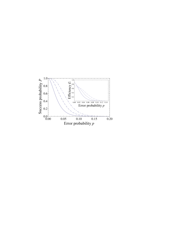
Figure 1: The probability that the error-corrected state is identical to the original state for different codes. The codes are assumed to have the parameters $[[64,56,3]]$ (solid), $[[64,48,5]]$ (dashed), and $[[64,43,7]]$ (dot-dashed). Inset the codes’ efficiency ${\cal E}$ is plotted.

In Fig. (1) we have also plotted, as an inset, the efficiency ${\cal E}$ v.s. the the single qubit error probability $p$. Here we see that as expected, for a fixed code length the smaller the error correction depth $t$, the more efficient the code is close to $p=0$. The codes with larger error correction depth $t$ are only more efficient than the codes with smaller $t$ when the error probability $p$ is substantial.

It has been known for some time now that efficient nondegenerate quantum codes exist for small errors. The efficiency increases with increased block length $k$ for a fixed error correcting depth $t$. In Fig. 2 we have plotted the efficiency ${\cal E}$ v.s. the single qubit error probability $p$ for existing codes correcting a single error, where, moreover, the codes $[[5,1,3]]$ and $[[85,77,3]]$ are perfect codes. This shows that long codes have the best efficiency, but only for a small range of error probabilities $p$ close to zero. The envelope of such a set of functions is actually the real point of interest, because it gives a bound for the efficiency of any depolarizing-channel, pure, nondegenerate code that is correcting only a single error per block.

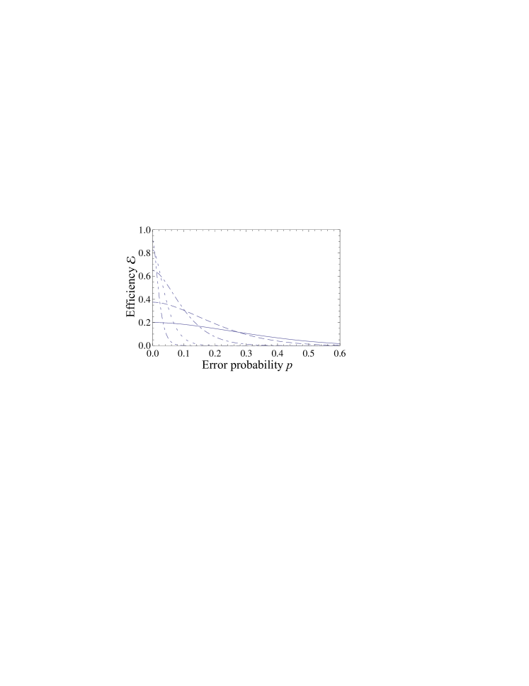
Figure 2: The efficiency for codes with assumed parameters $[[5,1,3]]$ (solid), $[[8,3,3]]$ (dashed), $[[17,11,3]]$ (dot-dashed), $[[40,33,3]]$ (small dashed), and $[[85,77,3]]$ (dot-dot-dashed).

Let us now compare the efficiency envelope functions of existing and hypothetical codes with an error correction depth of 1, 2, and 3, all having $n\leq 256$ in Fig. 3. To obtain these envelopes we plot the largest efficiency of the hypothetical codes fulfilling (2) and for $n\leq 128$ also the tabulated bounds in Grassl3 . It is trivially true that very close to $p=0$ the codes with the largest ratio $k/n$ for a given difference $n-k$ will have the highest efficiency. For larger $p$ this no longer holds true, so one needs to search trough a large number of hypothetical codes to make sure that one has found the most efficient code for any given $p$. A guiding principle in this search is that codes coming close to the Hamming bound are efficient as they use the code’s redundancy nearly optimally. The most efficient (each for some range of probabilities $p$), existing, single error correcting codes with $t=1$ and $n\leq 256$ are $[[5,1,3]]$ (perfect), $[[8,3,3]]$, $[[15,9,3]]$, $[[16,10,3]]$, $[[17,11,3]]$, $[[21,15,3]]$ (perfect), $[[40,33,3]]$, $[[74,66,3]]$, $[[85,77,3]]$ (perfect), $[[128,119,3]]$, and $[[256,246,3]]$. The implementation of these codes (and the codes below) can be found in calderbank2 ; Grassl3 , where the latter reference is the more extensive. The only hypothetical $t=1$ code we have found that could possibly beat any of these codes (but only in a small range of $p$) is a $[[170,161,3]]$ code, as shown in the Fig. 3 inset.

The $n\leq 256$ codes with $t=2$ which have the highest efficiencies are $[[11,1,5]]$, $[[16,4,5]]$, $[[18,6,5]]$, $[[27,13,5]]$, $[[30,16,5]]$, $[[35,20,5]]$, $[[58,42,5]]$, $[[70,54,5]]$, $[[128,110,5]]$ and $[[256,231,5]]$. Hypothetically, codes with the following parameters will be even more efficient: $[[14,3,5]]$, $[[16,5,5]]$, $[[17,6,5]]$, $[[27,15,5]]$, $[[39,26,5]]$, $[[83,68,5]]$, $[[118,102,5]]$, $[[170,151,5]]$, and $[[256,233,5]]$. The last two codes need an additional comment. The Hamming bound allows $[[170,153,5]]$ and $[[256,236,5]]$ codes, but an analysis of both existing and hypothetical codes with $n\leq 128$ shows that neither set of codes come close to saturating the Hamming bound. Both sets of codes have a nearly linear relationship between $k$ and $n$, so we have been a little bit conservative and estimated the last two hypothetical codes by linear extrapolation of the rest of the “hypothetical” set, and used these extrapolated parameters in plotting Fig. 3.

The most efficient, existing $t=3$ codes are $[[17,1,7]]$, $[[25,5,7]]$, $[[35,13,7]]$, $[[42,20,7]]$, $[[64,38,7]]$, $[[113,85,7]]$, $[[128,98,7]]$, and $[[255,215,7]]$. The hypothetical codes with higher efficiency are $[[20,3,7]]$, $[[22,5,7]]$, $[[28,11,7]]$, $[[36,18,7]]$, $[[59,39,7]]$, $[[94,72,7]]$, $[[121,98,7]]$, and $[[256,223,7]]$, where the last code again is inferred through linear extrapolation from the $n\leq 128$ codes in the corresponding set, whereas the quantum Hamming bound permits the code $[[256,229,7]]$.

In Fig. 3 one sees that, as expected, for sufficiently small errors $p$, the single-error correcting code is most efficient, whereas for larger $p$ it is conceivable that $t=2$ or $t=3$ codes could be more efficient. (Remember that so far we are considering hypothetical codes for $t>1$.)

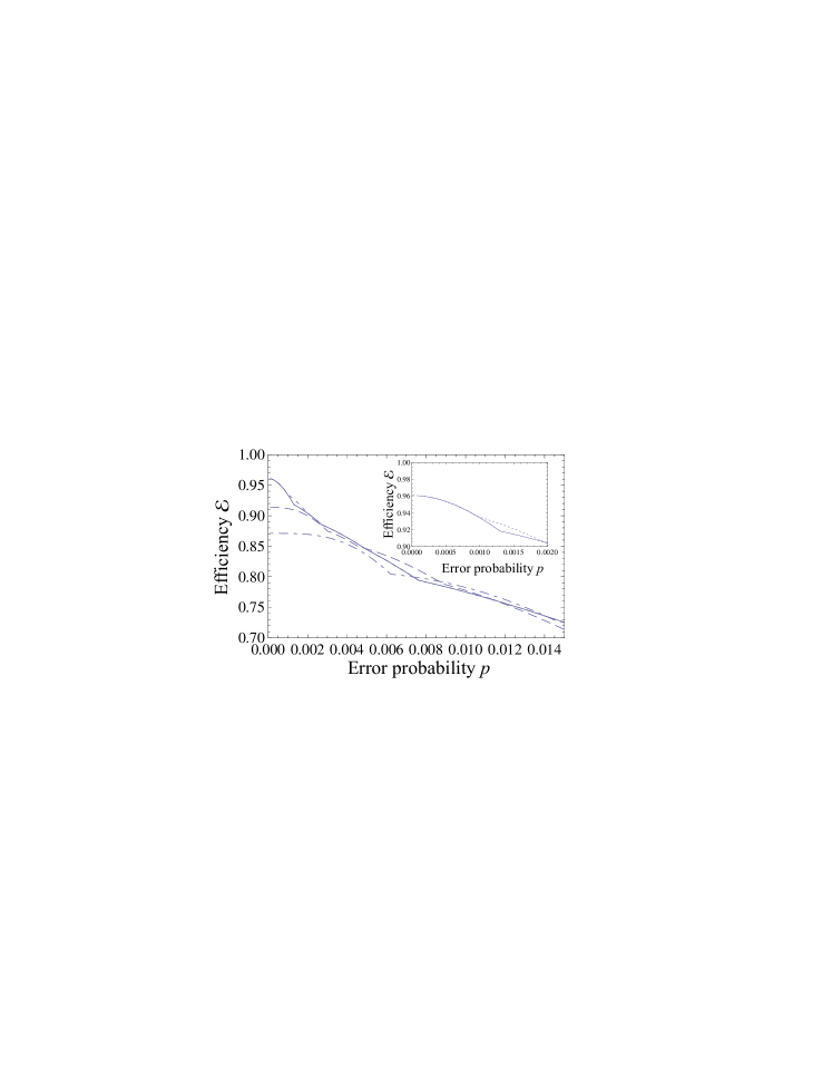
Figure 3: The maximum efficiency for hypothetical codes with assumed parameters $t=1$ (short-dashed), $t=2$ (dashed), $t=3$ (dot-dashed), and the most efficient existing codes with $t=1$ (solid). An enlargement of the plotted efficiency of existing and hypothetical codes with $t=1$ in the only region they differ is inset for clarity.

It is interesting to see for what interval of qubit error probabilities $0<p\leq p_{c}$ it is impossible to find $t>1$ codes that outperform the $t=1$ codes, given $\ \leq 256$. To find the interval we need to compute the qubit error probability $p_{c}$ for which the efficiency of the most efficient, existing $[[n,k_{1},3]]$ and the best hypothetical $[[n,k_{2},5]]$ codes are equal. To give an analytical estimate of the range $0\leq p\leq p_{c}$ where single error correcting codes are the most efficient we use Eqs. (7) and (8) and set ${\cal E}(n,k_{1},3,p_{c})={\cal E}(n,k_{2},5,p_{c})$. If we expand the ensuing expression to second order in $p_{c}$ and solve the equation, we find that

$$p_{c}\approx\sqrt{\frac{2(k_{1}-k_{2})}{k_{1}n(n-1)}}.$$ (9)

Since the difference $k_{1}-k_{2}$ grows only very slowly with $n$, but $k_{1}$ grows approximately linearly with $n$, we conclude that for $0<p\leq p_{c}$, where $p_{c}\sim n^{-3/2}$, there will exist a nondegenerate, length $n$, single qubit correcting code with higher efficiency than any length $n$, two-qubit correcting code. Using the values of $n$, $k_{1}$ for the existing code $[[256,246,3]]$ and $k_{2}$ for the hypothetical code $[[256,233,5]]$, we find that the range of error probabilities where the former code outperforms the latter is $0<p\leq 0.0013$. A more conservative estimate through the quantum Hamming bound, which allows a $[[256,237,5]]$ code, gives the bound $0<p\leq 0.0011$. This range of probabilities is surprisingly large.

However, as seen in Fig. 3, before the respective curves for the $[[256,246,3]]$ and $[[256,233,5]]$ codes above cross, the existing $[[128,119,3]]$ code becomes more efficient. Therefore, it is only for approximately $p\geq 0.0025$ any (so far hypothetical) $t>1$ code become more efficient than any (existing) $t=1$ code.

V How good are existing codes?

In Fig. 3, inset, the efficiency of the most efficient, existing, nondegenerate codes correcting one-qubit errors and the efficiency of the most efficient similar hypothetical codes is plotted. As mentioned above we have found only one hypothetical code that in a small range of error probabilities could outperform the existing codes, so there is little hope for improvement for the $t=1$ codes. One may ask why this is, and the answer is that the existing $t=1$ codes listed in the previous section all lie very close to the quantum Hamming bound which provides the least restrictive necessary condition for nondegenerate codes. E.g., the $[[256,246,3]]$ code uses 769 out of the possible 1024 syndrome vectors to correct all single qubit errors. That is, the code uses most of its redundancy to perform the task it is intended for – to correct the most frequent errors. We shall see below that in the range of error probabilities where a specific code is the most efficient, it is impossible to design more than a marginally more efficient code, even under the most optimistic assumptions. The nondegenerate perfect codes are simply perfect. They use all redundancy for the intended purpose.

In Fig. 4 we plot the maximum efficiency of $n\leq 256$ existing nondegenerate codes, listed in the previous section. Whereas it is quite trivial that for hypothetical codes, there must always be some small range of $p$ were a single-qubit correcting code must be more efficient than any $t>1$ code, given that they all have a maximum code length $n_{{\rm Max}}$, the result for existing codes is nontrivial. For the existing $n\leq 256$ codes we have analyzed, one can always find among them a $t=1$ code that has equal or higher efficiency for any value of the qubit error probability $p$ than any existing $t>1$ code. The reason for this counterintuitive result, that contradicts our experience from classical codes, is that the number of errors increases a factor $3^{t}$ faster for the Pauli channel than for e.g., a classical flip channel. Therefore, the redundancy must also grow much faster for a Pauli-channel code than for a classical bit-flip code. This makes the efficiency smaller for the $t>1$ than for the $t=1$ codes.

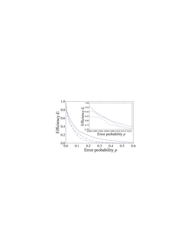
Figure 4: The efficiency for some existing codes with $n\leq 256$ vs. the qubit error probability $p$ for $t=1$ (solid), $t=2$ (dashed), and $t=3$ (dash-dotted).

VI Can existing codes be improved?

We have seen above that, excluding the three perfect codes, even the optimal codes do not use all possible syndromes. One may then ask how much could be gained if, hypothetically, the whole syndrome vector space could be used for correcting errors. One should remember that quite obviously the most frequent errors should be corrected with the highest priority, so before attempting to correct any double errors, one should correct all single errors etc., and it is on this premise codes are designed. However, in order to argue that existing codes cannot be much better, let us assume for the moment that codes that are pure, nondegenerate and that uses every syndrome to correct errors can be constructed. The number $r$ of “left over” syndrome vectors of a $[[n,k,2t+1]]$ code is

$$r=2^{(n-k)}-\sum_{i=0}^{t}3^{i}\left(\begin{array}[]{c}n\\ i\\ \end{array}\right)$$ (10)

and only for perfect codes this number is zero. The number $q$ of unique errors of order $t+1$ is

$$3^{t+1}\left(\begin{array}[]{c}n\\ t+1\\ \end{array}\right).$$ (11)

Hence we can correct a ratio $r/q$ of the $t+1$ order errors. If we corrected all such errors, the success probability $P$ would be boosted by the term

$$\left(\begin{array}[]{c}n\\ t+1\\ \end{array}\right)(1-p)^{(n-t-1)}p^{(t+1)}.$$ (12)

Because the number of leftover syndromes $r$ is smaller than the number of $t+1$ order errors (if not, the code is ill designed as it has sufficient length and redundancy to correct all errors of order $t+1$) we can not, even in the best case, correct all of them, and therefore the additional contribution to the success probability $P$ will be

$$\frac{r}{q}\left(\begin{array}[]{c}n\\ t+1\\ \end{array}\right)(1-p)^{(n-t-1)}p^{(t+1)}=\frac{r}{3^{(t+1)}}(1-p)^{(n-t-1)}p^{(t+1)}$$ (13)

and the additional contribution to the efficiency ${\cal E}$ will be $k/n$ times this number.

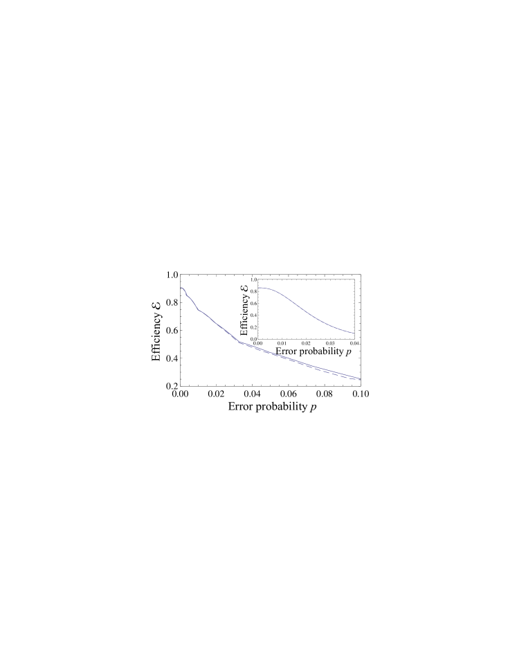
Figure 5: The efficiency for existing $t=2$ codes with $n\leq 256$ (dashed), and for assumed codes of the same lengths that uses every syndrome for error correction (solid), vs. the qubit error probability $p$. Inset the performance of the existing $[[128,110,5]]$ code (dashed) and an assumed pure, nondegenerate code with the same $n$ and $k$ that uses every syndrome for error correction (solid) are plotted.

To put these equations in context, let us take the $[[128,110,5]]$ code over GF(2*2) Grassl3 as an example. The code allows $2^{(128-110)}=262144$ syndromes, whereof 1 is needed to identify the no error case, $3\cdot 128=384$ are needed to identify all single errors, and $3^{2}\cdot 128\cdot 127/2=73152$ are needed to identify all double errors. Remain $r=262144-73537=188607$ syndrome vectors that can be used to correct some of the the $m=9217152$ triple errors. Hence, the efficiency can be boosted by a term $188607\cdot 110(1-p)^{125}p^{3}/(128\cdot 3^{3})\approx 6003(1-p)^{125}p^{3}$ which looks large, but which vanishes quickly when $p<(6003)^{-1/3}\approx 0.055$. This result is intuitive, because if already the probability for single errors is small, it will certainly not pay to correct triple errors (which will have a vanishingly small probability to occur). In Fig. 5, inset, we have plotted the efficiency of the code $[[128,110,5]]$ used as intended to correct up to double errors (dashed), and the efficiency of a similar length code where we have assumed that, in addition to all errors up to second order, we could use the 188 607 “left over” syndrome vectors to identify and correct this number of triple errors. However, as both the fraction of correctable triple errors is small, and for small values of $p$ the probability of triple errors is small, the two curves are almost identical and the difference can hardly been seen within the resolution of the figure. Moreover, as can be deduced from Fig. 4, inset, the $[[128,110,5]]$ code is no longer the most efficient code for error probabilities $p>0.01$, but the shorter code $[[70,54,5]]$ is more efficient. In Fig. 5 we have plotted most efficient $t=2$ existing codes with (dashed) and without (solid) the (with all likelihood overoptimistic) assumption that all $r$ “left over” syndrome vectors can all somehow be used to correct triple errors. There is little difference between the two curves, in particular for $p<0.01$. This suggests that current nondegenerate codes cannot be improved more than very marginally.

VII A comment on fidelity, efficiency and mutual information

As mentioned in Sec. III the best measure of a code’s efficiency would be based on the mutual information between the original and the corrected qubits. However, the mutual information is cumbersome to compute, so instead, the fidelity is often used. We have instead used a measure based on the success probability, and the reason therefore warrants a short comment.

After coding, and depolarization, a coded qubit block will belong to one of three categories: (1) It may have suffered $\leq t$ errors and therefore have a syndrome which will be recognized as correctable. After the recovery operation one will have the desired, original qubit block. (2) It may have suffered $>t$ errors and have a syndrome that is orthogonal to all syndromes of recoverable errors. (3) It may have suffered $>t$ errors but have a syndrome that is nonorthogonal to some syndromes of recoverable errors. The syndrome vectors will then occasionally be recognized as correctable. However, the recovery operator, intended for syndromes from group (1), will then in general not “generate” the desired qubit block but an erroneous one.

If we want to optimize the fidelity we should process the noncorrectable errors belonging both to group (2) and (3) in some manner and produce a proper length qubit block. While it is probably not the optimum operation, we could, e.g., project all these state onto the $k$ qubit (properly normalized) identity operator. This operator has a fidelity $2^{-k}$ to any pure initial $k$ qubit block, so the states in both group (2) and (3) will increase the fidelity if processed this way (if not by much), both from a mathematical and an experimental viewpoint.

On the contrary, neither of the groups (2) or (3) contribute to the success probability, as defined. In an experiment, one should therefore “throw away” any state with a syndrome orthogonal to those that signals a correctable error. This will rid us of group (2). Those times the syndromes of states belonging to group (3) are measured as recoverable, one must go ahead with the procedure, for there is no way one can decide if such an outcome is triggered by a state from group from (1) or from group (3). If it is from the latter group, the thus “recovered” state will with high likelihood be incorrect but such events will still contribute (very, very marginally) to the measured (but not to the computed) success probability.

However, whereas all states in group (1) contribute positively to the mutual information, the states in group (2) and those events that yields a ‘nonrecoverable” syndrome measurement in group (3) will with all likelihood contribute negatively because in general they will result in an incorrect qubit block. Therefore, it seems like the best strategy will be to discard these states. If so, they don’t contribute to the mutual information. However, the group (3) states that leads to a measurement event signalling a recoverable error are inevitably going to contribute negatively to the mutual information because they will result in a small portion of erroneous qubit blocks randomly mixed with the successfully recovered qubit blocks from group (1). We believe that this negative contribution will be small, in particular for long codes, for two reasons. The first reason is that even for quite large qubit error probabilities $p$, most states will belong to group (1), that is come out as the desired qubit blocks, provided that one uses a code that has the optimal efficiency for the particular error probability. E.g. the success probability of the code $[[128,119,3]]$ is 0.93 at $p=0.0035$ (at which point its efficiency is superseded by the $[[85,77,3]]$ code). Hence, “false corrections” at this error probability can come only from a (small) fraction of the 7 percent of blocks that have two or more errors. The second reason is that for long codes, the code qubit space dimension $2^{n}$ is much larger than the correctable syndrome sub-space with dimension $\leq 2^{k}$. Therefore, the overlap between a state in group (1) in the latter space and a state in group (3) in the former but not in the latter space will with all likelihood be very small. “False corrections” should hence be very rare for long codes.

From the considerations above we see that some strategies that serve to increase the fidelity actually decreases the mutual information. This is not so with success probability. We conjecture that the estimate of mutual information that can be derived from the success probability is rather close to the actual mutual information, although we have been unable quantify this conjecture. At any rate, it seems like fidelity, in spite of its popularity, is the worst of these three measures from this point of view.

VIII Conclusions

We have looked at pure, nondegenerate quantum-error correction codes for blocks of qubits subjected to statistically independent noise in a depolarizing channel. For a fixed maximum code length $n$ and a probability of error below a certain level, the codes that correct only a single error per block are the most efficient in the “steady state”, i.e., when the number of qubits to be transmitted is $\gg n$. We believe that in analogy with classical error correction, the hardware-implementation penalty in cost and complexity will be prohibitive for long codes. Therefore it is reasonable to compare codes of the same maximum length.

We have subsequently derived an approximate expression for the maximum qubit error rate where single quantum-error correcting codes will have the highest efficiency for a given length $n$ and found that if the error probability is at most $p\approx 10^{-3}$, then for a code length $n\leq 256$ it is not efficient to correct more than a single error even if more efficient nondegenerate, multiple-error correction codes will be invented. The range is surprisingly wide. Moreover, if the efficiency of nondegenerate, multiple error correcting codes will not improve by the invention of new codes, then the single-error correcting codes are most efficient regardless of the qubit error probability if one restricts the code length. This came as a surprise for us, but is good news for quantum information technology because as mentioned above, the number of errors, and hence the needed correction apparatus, grows exponentially with the correction depth. For example, the number of single errors per block grows as $3n$, whereas the number of double errors grows as $9n(n-1)/2$.

We have also provided evidence that the existing codes are close to optimal in performance. It hence seems unlikely that work on optimization of the codes considered (pure and nondegenerate for Pauli channels) will lead to more than very marginal improvements.

It is interesting to ask if the conclusions we have drawn above spill over to other channel models and to degenerate codes. To the best of our knowledge the answers to these questions are not known. We should suspect that for nondegenerate codes the result should hold even for other channels, for the general scaling behavior of such codes for $n$, $k$, and $t$ is similar. How the efficiency of degenerate codes behaves as a function of error correction ability is still an open question.

We have also not coupled the codes’ efficiency with its fault tolerance, and to the best of our knowledge the efficiency v.s. the fault-tolerance threshold is still an open question. Rather fault-tolerant codes are known Knill2 , but at the price of a significant overhead (a ratio $k/n\ll 1$). To make such a study, it is necessary to couple the qubit error probability to the gate error rate and the gate number, for codes of different correction depth $t$. So far, the investigated codes for fault-tolerant quantum computing typically has a rather small number of coded qubits $k$, and efficiency has been sacrificed for achieving a high fault tolerance.

References

- (1) For an introduction to quantum computing, see e.g., M. Nielsen and I. Chuang, Quantum Computation and Quantum Information (Cambridge University Press, Cambridge, 2000).
- (2) P. W. Shor, Phys. Rev. A 52, R2493 (1995).
- (3) A. M. Steane, Phys. Rev. Lett. 77, 793 (1996).
- (4) A. M. Steane, Phys. Rev. A 54, 4741 (1996).
- (5) A. R. Calderbank and P. W. Shor, Phys. Rev. A 54, 1098 (1996).
- (6) A. M. Steane, Proc. Roy. Soc. Lond. A 452, 2551 (1996).
- (7) C. H. Bennett, D. P. DiVincenzo, J. A. Smolin, and W. K. Wootters, Phys. Rev. A 54, 3824 (1996).
- (8) E. Knill and R. Laflamme, Phys. Rev. A 55, 900 (1997).
- (9) D Kribs, R. Laflamme, and D. Poulin, Phys. Rev. Lett. 94, 180501 (2005).
- (10) A. Ekert and C. Machiavello, Phys. Rev. Lett. 77, 2585 (1996).
- (11) R. Laflamme, C. Miquel, J. P. Paz, and W. H. Zurek, Phys. Rev. Lett. 77, 198 (1996).
- (12) D. Gottesman, Phys. Rev. A 54, 1862 (1996); A. R. Calderbank, E. M. Rains, P. W. Shor, and N. J. Sloane, Phys. Rev. Lett. 78, 405 (1997).
- (13) A. M. Steane, e-print arXiv:quant-ph9802061v2.
- (14) D. Gottesman, Phys. Rev. A 54, 1862 (1996).
- (15) D. Gottesman, e-print arXiv:quant-ph9607027.
- (16) R. Cleve and D. Gottesman, Phys. Rev. A 56, 76 (1997).
- (17) M. B. Plenio, V. Vedral, and P. L. Knight, Phys. Rev. A 55, 67 (1997).
- (18) D. W. Leung, M. A. Nielsen, I. L. Chuang, and Y. Yamamoto, Phys. Rev. A 56, 2567 (1997).
- (19) E. M. Rains, R. H. Hardin, P. W. Shor, and N. J. A. Sloane, Phys. Rev. Lett., 79, 953 (1997).
- (20) M. Grassl, Th. Beth, and T. Pellizzari, Phys. Rev. A 56, 33 (1997).
- (21) A. R. Calderbank, E. M. Rains, P. W. Shor, and N. J. A. Sloane, IEEE Trans. Info. Theory, 44, 1369 (1998).
- (22) A. M. Steane, IEEE Trans. Info. Theory 45, 1701 (1999).
- (23) E. M. Rains, IEEE Trans. Info. Theory 45, 1827 (1999).
- (24) E. M. Rains, IEEE Trans. Info. Theory 45, 266 (1999).
- (25) S. L. Braunstein, C. A. Fuchs, D. Gottesman, and H.-K. Lo, IEEE Trans. Info. Theory, 46, 1644 (2000).
- (26) E. M. Rains, Finite Fields Appl., 6, 146 (2000).
- (27) A. Ashikhmin, S. Litsyn, and M. A. Tsfasman, Phys. Rev. A 63, 032311 (2001).
- (28) E. M. Rains, IEEE Trans. Info. Theory 49, 1261 (2003).
- (29) A. S. Fletcher, P. W. Shor, and M. Z. Win, Phys. Rev. A 77, 012320 (2008).
- (30) J. A. Smolin, G. Smith, and S. Wehner, Phys. Rev. Lett. 99, 1 (2007).
- (31) M. Grassl, T. Beth, and T. M. Rötteler, Int. J. Quantum Inf. 2, 55 (2004).
- (32) M. Reimpell and R. F. Werner, Phys. Rev. Lett. 94, 080501 (2005).
- (33) N. Yamamoto, S. Hara, and K. Tsumura, Phys. Rev. A 71, 022322 (2005).
- (34) A. S. Fletcher, P. W. Shor, and M. Z. Win, Phys. Rev. A 75, 012338 (2007).
- (35) A. Ashikhmin and S. Litsyn, IEEE Trans. Info. Theory, 45, 1206 (1999).
- (36) A. Ashikhmin, A. M. Barg, E. Knill, and S. N. Litsyn, IEEE Trans. Info. Theory, 46, 789 (2000).
- (37) P. K. Sarvepalli, M. Rötteler, and A. Klappenecker, e-print arXiv:0804.4316.
- (38) P. W. Shor and J. A. Smolin, e-print arXiv:quant-ph9604006v2.
- (39) G. Smith and J. A. Smolin, Phys. Rev. Lett. 98, 030501 (2007).
- (40) M. Grassl, tabulated codes online available at http://www.codetables.de (2007). Accessed on 2008-10-07.
- (41) E. Knill, Nature 434, 39 (2005).