Phase-space structures I:
A comparison of 6D density estimators

Abstract

In the framework of particle-based Vlasov systems, this paper reviews and analyses different methods recently proposed in the literature to identify neighbours in six dimensional space (6D) and estimate the corresponding phase-space density. Specifically, it compares Smooth Particle Hydrodynamics (SPH) methods based on tree partitioning to 6D Delaunay tessellation. This comparison is carried out on statical and dynamical realisations of single halo profiles, paying particular attention to the unknown scaling, $S_{\rm G}$, used to relate the spatial dimensions to the velocity dimensions.

It is found that, in practice, the methods with local adaptive metric provide the best phase-space estimators. They make use of a Shannon entropy criterion combined with a binary tree partitioning and with subsequent SPH interpolation using 10 to 40 nearest neighbours. We note that the local scaling $S_{\rm L}$ implemented by such methods, which enforces local isotropy of the distribution function, can vary by about one order of magnitude in different regions within the system. It presents a bimodal distribution, in which one component is dominated by the main part of the halo and the other one is dominated by the substructures of the halo.

While potentially better than SPH techniques, since it yields an optimal estimate of the local softening volume (and therefore the local number of neighbours required to perform the interpolation), the Delaunay tessellation in fact generally poorly estimates the phase-space distribution function. Indeed, it requires, prior to its implementation, the choice of a global scaling $S_{\rm G}$. We propose two simple but efficient methods to estimate $S_{\rm G}$ that yield a good global compromise. However, the Delaunay interpolation still remains quite sensitive to local anisotropies in the distribution.

To emphasise the advantages of 6D analysis versus traditional 3D analysis, we also compare realistic six dimensional phase-space density estimation with the proxy proposed earlier in the literature, $Q=\rho/\sigma^{3}$, where $\rho$ is the local three dimensional (projected) density and $3\sigma^{2}$ is the local three dimensional velocity dispersion. We show that $Q$ only corresponds to a rough approximation of the true phase-space density, and is not able to capture all the details of the distribution in phase-space, ignoring, in particular, filamentation and tidal streams.

1 Introduction

There are many methods to analyse dark matter haloes structures. A standard approach involves investigating spherically averaged density profiles, such as the Hernquist profile [Hernquist 1990], the NFW profile [Navarro, Frenk and White 1997], the Moore profile [Moore et al. 1998, Moore et al. 1999] and the Stoehr profile [Stoehr 2006]. More sophisticated methods developed recently involve different elliptical density profiles [Jing & Suto 2002, Hayashi et al. 2007]. An other alternative consists of analysing velocity profiles, e.g., Romano-Diaz & van de Weygaert (2007), for a review.

Other investigations look in more details at halo detection as well as their internal substructures, the subhaloes. They usually use a two steps procedure: they first find haloes and substructures in position space, then use velocity information to apply binding criteria. Many such schemes are found in the literature, the simplest being the Friend-Of-Friend (FOF) algorithm [Huchra & Geller 1982]. More advanced methods rely for instance on the SKID algorithm [Stadel 2001] or on SUBFIND [Springel et al. 2001].

However, thanks to increased computational power, it now becomes possible to perform more detailed analyses that combine simultaneously velocity and position information. Indeed, modern simulations now reach enough resolution to identify structures and substructures in the full, six dimensional phase-space. Recent investigations in this topic studied phase-space dark matter profiles [Taylor & Navarro 2001], phase-space density estimation by using six dimensional Delaunay Tessellation (SHESHDEL) [Arad et al. 2004], or by using binary tree methods with smoothing (FiEstAS) [Ascasibar & Binney 2004], and a variety of different binary tree and six dimensional SPH methods with local adaptive metric in the EnBiD package [Sharma & Steinmetz 2006].

Two noticeable results were derived within these investigations: the measurement of a universal logarithmic slope for the phase-space density $f$ as a function of radius $r$, $f(r)\sim r^{-\alpha}$, with $\alpha\sim 1.875$ [Taylor & Navarro 2001], and the observation of a universal profile for the phase-space volume occupation function, $v(f)\propto f^{-2.5\pm 0.05}$ [Arad et al. 2004, Ascasibar & Binney 2004].

These results depend on the quality of the phase-space density estimators, a topic to which we devote this paper. We carefully analyse and cross compare the SHESHDEL, FiEstAS and EnBiD estimators.

This paper is organised as follows. Section 2 describes the various generic phase-space estimators and the corresponding concepts. We pay particular attention to the issue of the unknown scaling, $S_{\rm G}$, which relates position coordinates and velocity coordinates prior to the phase-space distribution function measurement. In Section 3 we test the phase-space estimators in three realisations of a halo profile: (i) a pure Hernquist isotropic halo, (ii) a composite Hernquist halo (a main Hernquist component with Hernquist subhaloes) and (iii) a halo extracted from a standard Cold Dark Matter (CDM) cosmological simulation. To have a better understanding of the results, more thorough analyses are performed in Section 4 focusing on (i) the local number of neighbours built by the Delaunay tessellation and on (ii) the local scaling between positions and velocities given by the adaptive metric of EnBiD. Section 5 shows the advantages of full phase-space analysis, with respect to more classical approaches such as the proxy $Q=\rho/\sigma^{3}$. Finally, Section 6 wraps up.

2 Phase-space density estimation

There are a few common approaches to measure six dimensional phase-space density, $f(\mathbf{x},\mathbf{v})$, for unrelaxed systems.

A straightforward method involves dividing phase-space into a Cartesian grid and approximating phase-space density by counting particles in each bin. While this clearly works quite well in three-dimensional space, it starts to be problematic in six dimensions. Even if we choose a poor quality resolution, e.g. $100$ bins along each axis, we get in the end a very large number of cells, e.g. $10^{12}$, and, for modern simulations with e.g. $10^{7}$ particles, almost all the cells will be empty. This basic example shows that for improved phase-space estimation, one needs to go well beyond the naive binning algorithm. Notice as well that to achieve a level of detail in phase-space comparable to what is usually obtained in position space, one needs a simulation with an extremely large number of particles.

A more sophisticated, frequently used method for density estimation in position space, uses smoothing with $k$ nearest neighbours found with standard tree techniques; it can be easily generalised to the six dimensional case. Assuming for the sake of simplicity that all particles have the same mass $m_{p}$, if, for each particle, $k$ neighbours are enclosed in a six dimensional ball of volume $V_{6}$, then the local phase-space density can for instance be measured with the simple following estimator, $m_{p}k/V_{6}$, which corresponds to a top hat kernel. In practice, more sophisticated kernels are used, i.e. each neighbour contributes to the measured density with a weight defined by a smooth function, usually a Smooth Particle Hydrodynamics (SPH) kernel. This kind of algorithm was proposed for phase-space density estimation by Sharma and Steinmetz (2006) (hereafter S06). It however requires the proper set up of a metric in six-dimensional space (velocity/position scaling).

In this paper we investigate more accurate algorithms developed recently in the literature, including improvements of the above SPH technique.

The first method, discussed in § 2.1, relies on six dimensional Delaunay tessellation (Arad et al., 2004; hereafter Arad04). The big advantage of this method is that it is parameter free, fully adaptive, while each particle has a natural neighbourhood. In practice, however, the Delaunay tessellation needs some additional smoothing. It is also very time and memory consuming [Arad et al. 2004, Weygaert & Shaap 2007]. It requires, similarly as the straightforward SPH method just mentioned above, a proper set up of a metric in six-dimensional space.

The second group of algorithms was proposed by Ascasibar & Binney (2004, hereafter A04) and improved by S06. The first step of their method, detailed in § 2.2, is simple and robust. Space is divided with the help of a binary tree into disjoint hyperboxes with one particle in each leaf node. Since each particle is in one hyperbox with volume $V$, its local phase-space density could be directly estimated from the equation $f=m_{p}/V$. Yet the phase-space density derived from this estimator is quite noisy: it is almost impossible to use it for practical purposes. Hence additional steps were proposed to make it useful. First, the binary tree may be improved with the help of a Shannon entropy criterion combined with boundary particles correction (S06). Secondly, some additional smoothing should be performed. There are few options to do so, as proposed by A04 and S06 and described in § 2.3, ranging from (a) a hyperbox smoothing following the philosophy of the SPH method, (b) a SPH method with a local adaptive metric, to (c) anisotropic SPH methods. The main advantage of this type of algorithm compared to the tessellation methods is time and memory consumption.

In the next sections, we describe each of these methods in turn and follow with a detailed discussion on the issue of position/velocity scaling (§ 2.4). The reader may refer to Table LABEL:table:algorithms and to the summary in § 6, if needed.

Table 1: The various 6D estimators tested in this paper

The estimator name	Description
SPH	Smoothing with spherical Epanechikov kernel using $N$ neighbours, global scaling
SPH-AM	Smoothing with spherical Epanechikov kernel using $N$ neighbours, local adaptive metric
ASPH-AM	Anisotropic smoothing with ellipsoidal Epanechikov kernel, using $N$ neighbours, local adaptive metric
FiEstAS	Smoothing with the hyperbox kernel, local adaptive metric
DTFE	Estimation from the Delaunay tessellation (equation 2), global scaling
smooth DTFE	Estimation from the Delaunay tessellation with spherical smoothing (equation 8), global scaling

2.1 The Delaunay Tessellation

The idea of using a Delaunay tessellation was primarily implemented to estimate density and velocity fields in cosmological simulations [Bernardeau & van de Weygart 1996, Schaap & van de Weygaert 2003]. The corresponding algorithm, called the Delaunay Tessellation Field Estimator (DTFE), was also used to demonstrate the advantages of the tessellation over SPH methods [Pelupessy et al. 2003]. In particular, the DTFE method better captures the abrupt transitions between regions of different densities and provides a better estimate for high densities.

The main parts of the DTFE algorithm were used by Arad04 to develop their six dimensional phase-space density estimator called SHESHDEL. Beside the position-velocity scaling problem that is addressed in § 2.4 and in § 4.2, the method itself is parameter free and presents well behaved statistical properties. Its main disadvantage is that it is computationally costly, although it scales like $N^{1.1}\log N$ (Arad, in preparation), where $N$ is the number of particles: the construction of a Delaunay tessellation of approximately $N\sim 10^{6}$ particles requires almost three days of calculation on a modern computer and the full output of $10^{9}$ Delaunay cells amount to $40$ GB of data in the end.

From a 6D Delaunay tessellation, it is easy to estimate the phase-space density, $f(\mathbf{x},\mathbf{v})$. Space is indeed partitioned into joint but non overlapping 6-dimensional polyhedrons - Delaunay cells, each one defined by 7 vertices. There is an unique 6 dimensional sphere passing through these 7 vertices, which by definition of the tessellation, does not encompass any other particle from the sample. Let $\{D_{i}^{1},D_{i}^{2},...,D_{i}^{N_{i}}\}$ be the $N_{i}$ Delaunay cells around particle $i$. We can define a macro Voronoi cell $W_{i}$ by joining all Delaunay cells containing particle $i$:

$$W_{i}=\bigcup_{j=1,...,N_{i}}D_{i}^{j}.$$ (1)

Then it is straightforward to define an estimate of the phase-space density for each particle $i$ of mass $m_{p}$ as:

$$f_{i}=7\frac{m_{p}}{\left|W_{i}\right|},$$ (2)

where $|W_{i}|$ is the volume of the macro cell and the factor $7$ accounts for the fact that each Delaunay cell contributes to the density of 7 particles. In practice, as mentioned earlier, the corresponding estimated phase-space density is very noisy, and one must introduce some additional smoothing. Let

$$f_{D_{i}}=\frac{1}{7}\sum_{j\in{D_{i}}}f_{j}\,,$$ (3)

be the average phase-space density defined for Delaunay cell $D_{i}$. One can then define a smoother phase-space density estimator as:

$$f^{\prime\prime}_{i}=\frac{\sum\limits_{j=1,...,N_{i}}f_{D_{i}^{j}}|D_{i}^{j}|}{\left|W_{i}\right|},$$ (4)

where $j$ indexes all Delaunay cells around particle $i$ and $|D_{i}^{j}|$ represents the volume of each Delaunay cell.

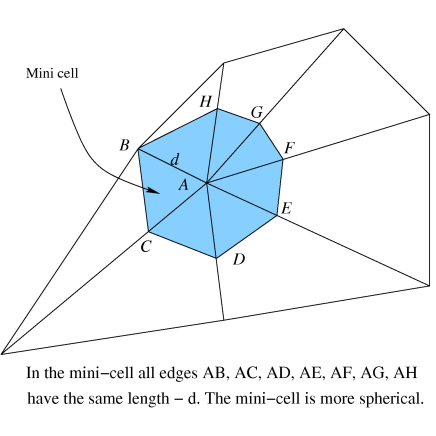
Figure 1: A method of smoothing which is appropriate for a Delaunay tessellation and corrects for local anisotropies: it involves redefining the local volume in such a way that one gets in the end a more spherical mini-cell.

For simulations without e.g. periodic boundaries, the phase-space density of particles near the edge of the computing domain can be underestimated. This is for instance the case when the sample has been cut from a bigger cosmological volume. To cope with this edge effect problem, one can introduce another definition for the smooth phase-space density estimator. Consider particle $i$, surrounded by its Delaunay cells $D_{j}$, and let $d$ be the distance between this particle and its closest neighbour (Figure 1). Then, the mini-cell around particle $i$ is defined as the collection of Delaunay cells $D^{\prime}_{j}$, which are similar to $D_{j}$ but are scaled in such a way that each edge in $D^{\prime}_{j}$ containing particle $i$ is exactly of length $d$. The volume of $D^{\prime}_{j}$ reads

$$|D^{\prime}_{i}|=|D_{i}|\prod_{j\in{D_{i}}}\frac{d^{6}}{|e_{ij}|},$$ (5)

where $|e_{ij}|$ is the length of the segment joining particle $i$ and $j$ in Delaunay cell $D_{i}$. As a result, a natural phase-space density estimator reads

$$f^{\prime\prime\prime}_{i}=\frac{\sum\limits_{j=1,...,N_{i}}f_{D_{i}^{j}}|{D^{\prime}}_{i}^{j}|}{\sum\limits_{j=1,...,N_{i}}|{D^{\prime}}_{i}^{j}|}.$$ (6)

However, it might be better to use linear interpolation to estimate the phase-space density in each mini-cell, to perform additional local noise filtering:

$$f_{D^{\prime}_{i}}=f_{D_{i}}+\frac{d}{7}\sum_{j\in{D_{i}}}{\frac{f_{i}-f_{j}}{|e_{ij}|}}.$$ (7)

In the end we can thus define a phase-space density estimator with interpolated density as follow:

$$f^{\prime}_{i}=\frac{\sum\limits_{j=1,...,N_{i}}f_{{D^{\prime}}_{i}^{j}}|{D^{\prime}}_{i}^{j}|}{\sum\limits_{j=1,...,N_{i}}|{D^{\prime}}_{i}^{j}|}.$$ (8)

The mini-cells are more regular and spherical, so both phase-space density estimators $f^{\prime}$ and $f^{\prime\prime\prime}$ are expected to be less sensitive to local fluctuations and local anisotropies due to noise and edge effects.

Note that all of the above smoothing methods are based on Natural Neighbour Interpolation techniques [Weygaert & Shaap 2007]. In what shall follow, although we studied all the estimators, $f_{i}$, $f^{\prime\prime}_{i}$, $f^{\prime}_{i}$ and $f^{\prime\prime\prime}_{i}$, we shall present explicit results only on $f^{\prime}_{i}$ (equation 8) and on $f_{i}$ (equation 2).

2.2 Tree partitioning

As discussed in the introduction of § 2, the main point of the algorithm FiEstAS  proposed by A04 and later improved by S04 in the EnBiD  implementation, is the division of space into a binary tree. In FiEstAS, the splitting axis is chosen alternatively between position space and velocity space, then in each of these respective subspaces, the axis with highest elongation, $\langle x_{i}^{2}\rangle-\langle x_{i}\rangle^{2}$, is split. This splitting criterion helps the cells to preserve a shape as cubic as possible.

However, a visual inspection of position and velocity diagrams of typical simulations (Figure 11) shows that position space contains more structures, and thus more information than velocity space. As a result, one can argue that for optimal accuracy, the splitting should occur more often in position space than in velocity space. This observation was used in the EnBiD algorithm to define a better splitting criterion. Before splitting occurs, one has to find the subspace (velocity or position) in which it should be performed. To do that, the Shannon entropy, $S$, is calculated after dividing each subspace into $N$ equal size bins:

$$S=-\sum_{i=1}^{N}\frac{n_{i}}{N}\log{\frac{n_{i}}{N}},$$ (9)

where $n_{i}$ is the number of particles in each bin. The subspace which has to be splitted is the one with smallest entropy. Finally, the direction of splitting is chosen again using the highest elongation criterion, to preserve a close to cubic shape.

As for Delaunay tessellation, correction for edge effects is crucial in the binary tree partition algorithm. To illustrate that point, it was shown in S06 that for $10^{6}$ particles uniformly distributed in a 6D spherical region, about $79\%$ of them lie near the border, compared to $5\%$ in the 3D case. This reflects the so called curse of dimensions. The natural shape of local border in the binary tree partition algorithm is an hypercube. When the data do not preserve locally this shape, the volume occupied by the boundary particles tends to be overestimated, hence their phase-space density tends to be underestimated. This bias is moreover expected to worsen and to propagate further away from the edges if additional smoothing is performed.

Both FiEstAS and EnBiD redefine borders to correct for edge effects. While FiEstAS does it only for the tree leaves, EnBiD applies the correction to all the nodes of the tree, in order to insure proper entropy calculation and to better estimate the phase-space density of small structures found in the halo.

2.3 Smoothing

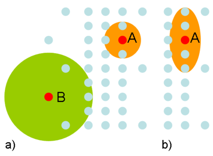
Figure 2: Biases in the SPH density estimation and potential advantages of anisotropic SPH methods: a) SPH method: density is underestimated for particle A and overestimated for particle B; b) ASPH method better traces local structures and should lead to better density estimation.

From these tree methods, one could estimate naively the phase-space density by exploiting directly the information stored in the tree structure, as argued in the end of the introduction of § 2, but measurements performed that way would be rather noisy: additional interpolation, should be applied to the data in order to achieve a good measurement of phase-space density. A04 and S06 investigated a few smoothing procedures, that we discuss now.

Let us first describe the smoothing method proposed by A04 (called later FiEstAS smoothing). The main idea comes from SPH techniques, but the smoothing kernel is a hyperbox rather than a hypersphere. This treatment avoids the need for a definition of a local metric. First, the mass of each particle is distributed uniformly over its leaf volume. Then, a hyperbox of volume $V_{s}$, centred on this leaf and with the same axis ratio, is found, such that it contains a mass $M_{s}$, which basically defines the kernel size. Local phase-space density is then calculated from the equation $f=M_{s}/V_{s}$. In our investigations, we shall use mainly the $M_{s}=2m_{p}$ value proposed by S06 (while A04 suggest $M_{s}=10m_{p}$).

The other approach uses a classic SPH technique. For our investigations, we shall use the Epanechikov kernel

$$W(x,h)=f_{d}\left\{\begin{array}[]{cc}\displaystyle 1-\sum_{i=1}6\left(\frac{x_{i}}{h_{i}}\right)^{2}\,,&0\leq{x_{i}}/{h_{i}}\leq 1\,,\\ 0\,,&{x_{i}}/{h_{i}}>1\,,\end{array}\right.$$ (10)

with an additional bias correction. As mentioned in S06, this estimator seems to give the best results for SPH phase-space estimation.

One of the disadvantages of the SPH method is the way it handles strong transitions between regions of very different densities, as illustrated by Fig 2a. The key point is that the SPH method is not able to capture correctly strong variations of the density local curvature. Because of the spherical shape of the kernel and the fixed number of neighbours used to perform the calculations, the density will be underestimated near the edge of the regions with higher density (particle A), or more generally in regions with significant negative local curvature. On the other hand the density will be overestimated near the edge of the low density regions (particle B), or in regions with significant positive local curvature. One way of resolving this issue, and of better capturing filamentary structures such as in Fig 2a, is to use an anisotropic SPH kernel, which adapts locally to the shape of structures and is thus more appropriate to capture to local curvature variations. First, the $N_{A}$ nearest neighbours are found for each particle, which allows one to compute a deformation tensor $H$, that is used to define a local ellipsoid with $N_{B}$ nearest neighbours (usually $N_{A}>N_{B}$). Each particle contained in this ellipsoid contributes to the phase-space density with the weights given by the SPH kernel, scaled properly to take into account the ellipsoid shape (Fig 2b).

Note that, in addition to the issues described in Figure 2, the density calculated with SPH methods presents some non trivial biases due to local Poisson shot noise which can in part be corrected for (see S06 for details).

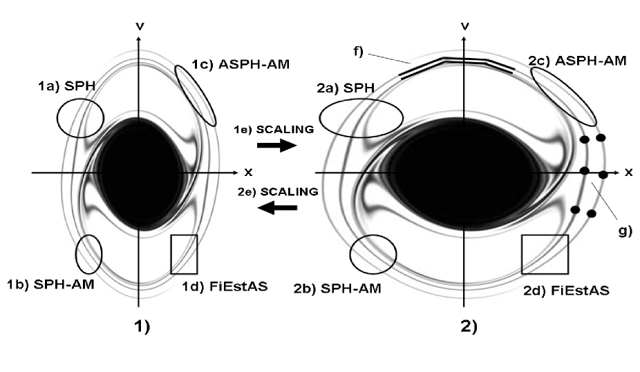
Figure 3: Illustration from a 2D simulation of Alard & Colombi (2005) of the velocity-position scaling and the various methods used to measure the coarse grained phase-space distribution function. 1) The left panel shows the phase-space distribution function in the “global” coordinate system used by the authors. 2) The right panel shows a scaled version of it in such a way that the same spread is observed in x and v coordinates. We call that a “local” system of coordinates as the scaling can be global as shown here, or local, as discussed in the main text. 1a) SPH spherical kernel in global coordinates, 2a) becomes ellipsoidal in local coordinates and is not optimal; 1b) SPH with a local Adaptive Metric presents an ellipsoidal kernel in global coordinates, 2b) but is set up in such a way that the kernel is spherical in local coordinates; 1c) Anisotropic SPH with a local Adaptive Metric in global coordinates, 2c) in local coordinates. 1d) FiEstAS smoothing in global coordinates 2d) presents a hypercubical kernel in local coordinates; f) local clouds resolve accurately phase-space structures, but g) particles from cosmological simulations only sparse sample them.

2.4 Position-velocity “metric” correction

There is a last one important problem that arises when one aims to estimate phase-space density. In order to perform some local phase-space density estimation, one needs to find a way to join position space and velocity space, or in other words to define a proper metric that allows one to estimate local distances and local volumes in phase-space. This generic problem does not have an obvious solution. Let us first discuss that issue and then detail the implementations to resolve it for the phase-space estimators used in this paper.

2.4.1 Coarse grained versus fine grained phase-space density

The dynamics of dark-matter is usually modeled by a self-gravitational collisionless fluid which follows the so called Vlasov-Poisson equations:

$$\frac{\mathrm{d}f}{\mathrm{d}t}\equiv\frac{\partial f}{\partial t}+\mathbf{v}\frac{\partial f}{\partial\mathbf{x}}-\frac{\partial\phi}{\partial\mathbf{x}}\frac{\partial f}{\partial\mathbf{v}}=0,$$ (11)

$$\nabla^{2}\phi(\mathbf{x},t)=4\pi G\int{f(\mathbf{x},\mathbf{v},t)\mathrm{d}\mathbf{v}}.$$ (12)

Because it is very difficult to solve these equations directly, the continuous fluid formulation is usually approximated by collisionless particles which follow the classical gravitational Newtonian equations, hence producing Monte Carlo realisations of this set, with additional softening to maintain the forces bounded. The most important question here is how this approximation affects the phase-space density properties. Liouville theorem states that the phase-space distribution function remains constant along trajectories of the system

$$f(\mathbf{x}(t),\mathbf{v}(t),t)={\rm constant}.$$ (13)

This is true for the smooth, fine-grained phase-space density $f$. In $N$-body simulations, it is in practice possible to probe only the coarse-grained phase-space density, $\bar{f}$, which is the average of $f$ over a small but finite volume [Binney & Tremaine 2008]. This quantity does not follow the Liouville theorem anymore because of mixing processes occurring at small scales [Tremaine et al. 1986, Arad et al. 2004]. Furthermore, the measurement of ${\bar{f}}$ depends highly on the way the coarse graining volume is defined, hence in particular on the local scaling to be applied to velocities versus positions. To have a proper measurement of ${\bar{f}}$ that approaches as much as possible the fine grained distribution function from the dynamical point of view, or some sensible local average of it, one would need the knowledge of the whole dynamical history of the system.

One way to overcome this problem is to solve numerically Vlasov’s equations using a more sophisticated approach than the simple $N$-body method, where the phase-space distribution function is modeled by small elements of metric, such as ellipsoid “clouds”, that sum up to a dynamically meaningful coarse grained version of the distribution function. This method is discussed in detail and applied in 1+1 D in Alard & Colombi (2005). Of course the generalisation of such a method to 6D is quite costly. However, a simple alternative, in the spirit of this method, would be to attach to each particle of a $N$-body simulation the information corresponding to the local phase-space volume (or the local metric), that would be followed during the evolution of the system [Vogelsberger et al. 2008]. Note that we then follow a sparse sampling of the fine grained distribution function as long as the dynamical effects due to the discrete particle representation are negligible. Then the appropriate shape for the phase-space element used to measure the coarse-grained distribution function would be given by a local average on a number of neighbouring particles in phase-space, as is achieved by the adaptive SPH method.

Finally, if such an information is not available, and without supplementary prior on the dynamical state of the system, one can just try to find the best coordinate transform that preserves local isotropy within the coarse grained volume. This method basically assumes that the systems evolved from a smooth distribution function. In that sense, for cold dark matter haloes, it only traces correctly the coarse distribution after relaxation to a quasi-steady state (i.e. a few dynamical times after collapse). Note that a simple application of this idea to find a global scaling between position and velocities basically produces the system of coordinates where the velocity scatter is of the same order of the positions scatter.

To illustrate this discussion, figure 3.1 shows one of the outputs of a 2D phase-space simulation of Alard & Colombi (2005), using the cloudy method (briefly sketched above). The system was evolved during approximately 40 dynamical times from an initial top-hat distribution function slightly apodized at the edges. Figure 3.2 shows the same realisation, but the position coordinate is scaled in such a way that both velocities and positions show the same spread: this is the natural system of coordinate for a global definition of the scaling to be used between positions and velocities prior to the definition of a small round coarse graining volume.

In the cold dark matter scenario, initial conditions can by approximated by a three dimensional sheet (small dispersion in velocity space) immersed in six dimensional phase-space, that subsequently evolves in time and gains a complex shape (without loosing its connectivity or volume as stated by the Liouville theorem). The equivalent of such a sheet in our 2D phase-space representation would be e.g. the curve (f), accurately followed by many cloud elements. As mentioned above, Vlasov-Poisson equations are usually numerically resolved relying on a particle representation. After many time steps, because of variations of the local force field, particles initially close by depart from each other (g). Mixing processes occur at small scales, and the phase-space sheet, poorly modeled by the particles, loses its fine structures. The way the coarse-grained phase-space density $\bar{f}$ is calculated is shown on e.g. (2d). The use of a finite local volume for computing $\bar{f}$ results in the averaging of the phase-space density over many curves – or sheets in six dimensions. From now on, unless otherwise stated, we shall skip the bar and use the $f$ symbol for the coarse-grained phase-space density.

2.4.2 Solutions for the position-velocity scaling

Inspired by the discussion in previous paragraph, we now propose two ways of fixing the position-velocity scaling:

• A global scaling factor between positions and velocities, that will be applied to the standard SPH and Delaunay Tessellation algorithms. This global factor tries to make the phase-space distribution function globally isotropic, i.e. with the same spread in velocities and in positions.

• A local scaling factor that depends on phase-space coordinate $(x,v)$, and that tries to make the phase-space distribution function locally isotropic. This local scaling factor is implemented by construction in FiEstAS and its improvement, EnBiD, as detailed below. It will be used as well when additional smoothing is performed with SPH or ASPH techniques. In that case we shall denote the methods by SPH-AM and ASPH-AM, respectively.

(i) Global scaling:

For the global scaling method depending on one parameter, $S_{\rm G}$, the metric transform can be written in the form:

$$\left(\begin{array}[]{c}dx^{\prime}\\ dv^{\prime}\end{array}\right)=\left(\begin{array}[]{cc}{1}/{\sqrt{S_{\rm G}}}&0\\ 0&\sqrt{S_{\rm G}}\end{array}\right)\left(\begin{array}[]{c}dx\\ dv\end{array}\right).$$ (14)

We test here two different ways of setting $S_{\rm G}$, that apply to single dynamical systems, such as the cold dark matter haloes analysed in this paper. Such a global scaling finds a transformation that changes for instance Fig. 3.1 in Fig. 3.2.

The first scaling uses simple dynamical arguments that lead to a comparable scatter in velocity and position space of the phase-space distribution function, or in other worlds to a “more round” shape of the cloud representing $f(x,v)$. It relies on the fact that dark matter haloes are known to be well fitted by the NFW profile [Navarro, Frenk and White 1997]. In particular, within that model, we use the relation

$$r_{200}=\frac{v_{200}}{10H(z)},$$ (15)

where $r_{200}$ and $v_{200}$ are the viral radius and the viral velocity of the halo, respectively, and $H(z)$ is the Hubble constant in units of $\mbox{km}~{}\mbox{s}^{-1}~{}\mbox{kpc}^{-1}$ [Schneider, 2006]. For the haloes analysed in this paper, $z=0$ and $H(0)=0.1h$. In that case, the natural set of coordinates, that fixes properly the global scaling between positions and velocities, simply uses distances expressed in units of kpc $h^{-1}$ and velocities in km s^-1. In this case the global scaling is set to $S_{I}=1.0h\mbox{ km}~{}\mbox{s}^{-1}~{}\mbox{kpc}^{-1}$.

The second method, more sophisticated, should reach approximately the same scaling. It involves attempting to enforce global isotropy of the distribution of particles in phase-space. To achieve that, the distances of each particle to its closest neighbour in position subspace and in velocity subspace, are computed, which allows us to estimate the probability distribution functions of these distances, $p(r)$ and $p(v)$. The global scaling $S_{\rm dist}$ between the two subspaces is the one where the maximum of $p(r)$ and the maximum of $p(v)$ coincide.

(ii) Local scaling:

Obviously, although it presents the advantage of being simple to implement and robust, the global scaling is not optimal. However, it is possible to enforce, to some extent, local isotropy of the phase-space distribution function by examining the local neighbourhood of each particle, as is implemented in the FiEstAS and EnBiD algorithms.

In FiEstAS the natural local scaling $S_{\rm L}$ between velocity subspace and position subspace is simply determined from the axis ratio of the tree leaf containing the particle (which is equivalent to pass from Figure 3.1d to Figure 3.2d). By construction of the tessellating tree, the local isotropy between both subspaces should be preserved in the first approximation, as the calculation of the final smoothing hyperbox preserves this axis ratio. For the modification of FiEstAS proposed by the EnBiD algorithm, the splitting of the binary tree is improved by the calculation of Shannon entropy, which in principle warrants a better local assignment of the metric frame.

Finally one can perform additional SPH or Anisotropic SPH interpolation in the local metric frame determined by EnBiD, that lead to our SPH Adaptive Metric algorithms (SPH-AM and ASPH-AM). Prior to SPH or ASPH interpolation, the phase-space coordinates are scaled in such a way that the local hyperbox corresponding to the leaf containing the particle becomes hypercubical (Figure 3.1d to Figure 3.2d, to obtain Figure 3.2b and Figure 3.2c). Of course the biases expected in SPH and ASPH interpolations mentioned in the end of § 2.3 are still present, even with this local metric approach.

To summarise, we see that FiEstAS method with EnBiD improvement corresponds to hyperbox smoothing with adaptive metric. The only thing that changes between SPH-AM or ASPH-AM is the shape of the kernel used to perform the smoothing.

3 Numerical experiments

3.1 Hernquist profile

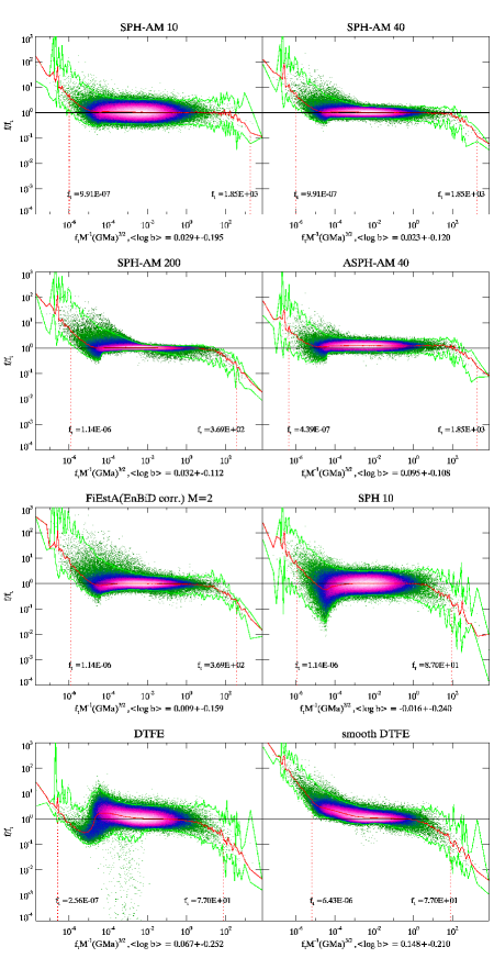
Figure 4: The ratio $b=f/f_{t}$ between the measured phase-space distribution function, $f$, and the analytical value, $f_{t}$, as a function of $f_{t}$, derived for an isotropic Hernquist profile and different smoothing methods as indicated on the top of each panel. From left to right and top to bottom, (a) SPH with local Adaptive Metric and 10 neighbours, (b) SPH with local Adaptive Metric and 40 neighbours, (c) SPH with local Adaptive Metric and 200 neighbours, (d) Anisotropic SPH with local Adaptive Metric and 40 neighbours, (e) FiEstAS algorithm with EnBiD improvement and $m_{p}=2.0$, (f) SPH with 10 neighbours, (g) DTFE method and (h) DTFE with spherical sphere smoothing. These two dimensional histograms are calculated using 400x400 logarithmic bins. The central curve corresponds to the median value of $b$ calculated over 200 logarithmic bins along the $x$ axis, taking into account only bins containing 2 particles or more. The two additional curves on each side show $3$ sigma errors estimated from the dispersion above and below the median curve. The two dashed vertical lines mark the range for which the median departs by more than a factor 5 from $f_{t}$. The mean log-ratio $\langle\log b\rangle$ and its dispersion, $\sigma=\sqrt{\langle(\log b-\langle\log b\rangle)^{2}\rangle}$, are indicated on each panel and were computed using all the data.

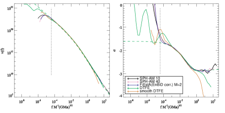
Figure 5: Hernquist profile: measurement of $v(f)$ (left) and its logarithmic slope (right) with different phase-space estimators. The dashed line corresponds to the analytical solution. The vertical dashed line marks the value $\log f_{\rm min}=-4.41$, corresponding to the cut-off of the halo at $5$ virial radii.

In order to test the various above described methods, we first examine control “phase mixed” samples for which there are analytical solutions. Hence, we follow A04 and S06 and generate a Hernquist isotropic profile [Hernquist 1990]. In that case, the projected density distribution is given by

$$\rho(r)=\frac{1}{2\pi 3}\frac{M}{(r/a)(1+r/a)^{3}},$$ (16)

where $M$ is the halo total mass and $a$ is a scale length. We follow exactly the prescriptions of A04 and S06 to create a random set of positions and random velocities obeying the appropriate distribution, relying on the fact that in this model, the phase-space density distribution function, $f$, depends only on energy $E$,

$$E=\frac{v^{2}}{2}+\phi(r)=\frac{v^{2}}{2}-\frac{GM}{a}\frac{1}{1+r/a},$$ (17)

where $r$ and $v$ correspond to position and velocity, respectively. At equilibrium, the distribution function reads

$$f_{t}(E)=M\frac{3\sin^{-1}(q)+q\sqrt{1-q^{2}}(1-2q^{2})(8q^{4}-8q^{2}-3)}{4a^{3}\pi^{3}(2GM/a)^{3/2}(1-q^{2})^{5/2}},$$ (18)

with

$$q=\sqrt{-\frac{E}{GM/a}}.$$ (19)

In order to have a halo with realistic properties, we would like it to follow equation (15), i.e. $v_{\rm vir}=S_{I}r_{\rm vir}$ (in our case $r_{\rm vir}\simeq r_{200}$), with $S_{I}=1.0h\mbox{ km}~{}\mbox{s}^{-1}~{}\mbox{kpc}^{-1}$. The circular velocity of the Hernquist profile reads

$$v_{\rm cir}(r)=\frac{\sqrt{GMr}}{r+a}.$$ (20)

Combining this equation taken at the virial radius with equation (15) gives the total halo mass

$$M=\frac{h^{2}a^{3}c(c+1)^{2}}{G}.$$ (21)

In practice, the profile is also cut-off at a radius $r_{\rm cut}$, i.e. all the particles verify $r<r_{\rm cut}$. In what follows, a concentration parameter $c$ is defined such that $r_{\rm vir}=ca$, where $r_{\rm vir}$ is the virial radius.

For our test sample, we take $5\cdot 10^{5}$ particles, $r_{\rm vir}=320$ kpc, $r_{\rm cut}=5r_{\rm vir}$, $h=0.7$ and $c=4$. For both the Hernquist profile and the Hernquist composite profile (next subsection), we measure $f$ in units of $M^{-1}(GMa)^{3/2}$. This choice of parameters was meant to compare directly our measurements with S06. Note however that our value of $r_{\rm cut}$ is much smaller than that of S06, to make DTFE method tractable. Without such a cut-off, we would indeed have too many neighbours for the particles near the edge. This abrupt cut-off might a priori introduce some contamination for $f\la f_{\rm min}$, where $f_{\rm min}$ is the value of the phase-space distribution function at $r=r_{\rm cut}$ and $v=0$ ($\log f_{\rm min}=-4.41$ in our units). Yet, we have checked, by taking very large values of $r_{\rm cut}$ that our implementation of the EnBiD estimator is quite consistent with that of S06.

Figure 4 shows the ratio $b=f/f_{t}$ between the estimated phase-space density $f$ and the analytical result, $f_{t}$ given by equation (18), as a function of $f_{t}$, for various smoothing methods, as indicated on the top of each panel.

For SPH-AM with $10$ neighbours, we get a good approximation of $f_{t}$ over about $9$ decades delimited by the two vertical dashed lines. These lines correspond to a five fold relative error on the determination of the phase-space density compared to the exact solution. With $40$ neighbours, the spread drops down by almost a factor of $2$, but at the cost of a narrower available dynamic range, because of the bias introduced by the softening of the sharp transitions between overdense and underdense regions and nearby local extrema (see also the discussion in § 2.3). This effect is therefore even more prominent for SPH-AM $200$. The FiEstAS algorithm with EnBiD improvement and $m_{p}=2.0$ gives a spread comparable to SPH-AM with around $20$ particles, but the range of accurate phase-space estimation is smaller as there is a noticeable bias in the high density region. For Anisotropic SPH-AM, $64$ particles are used to find the best fitting local ellipsoid while softening is performed over $40$ particles. In this case, the plot looks almost the same as for SPH-AM with a small overall systematic overestimation of the true phase-space density, which remains despite the kernel bias correction.

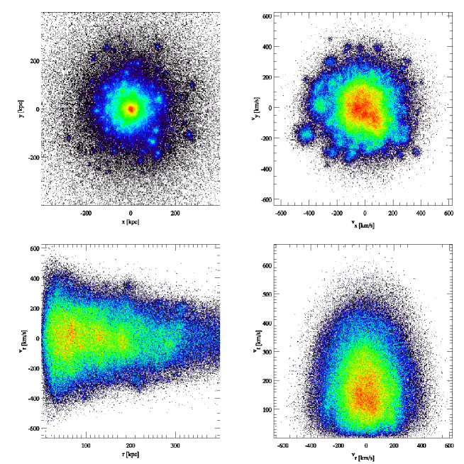
Figure 6: the Hernquist profile with substructures in phase-space. Upper left panel: $x$–$y$ position space; upper right panel: $v_{x}$–$v_{y}$ velocity space; lower left panel: phase-space diagram, radius $r$–radial velocity $v_{r}$; lower right panel: radial velocity $v_{r}$–tangential velocity $v_{t}$. Each plot is a two dimensional histogram with $400\times 400$ bins. Only the central part of the halo is shown here.

For DTFE and standard SPH methods, we have to set the global position-velocity scaling factor $S_{\rm G}$, where $v=S_{\rm G}r$. We use the two methods described in part (i) of § 2.4.2. The first one gives $S_{\rm G}=S_{I}=1.0h\mbox{ km}~{}\mbox{s}^{-1}~{}\mbox{kpc}^{-1}$ while the second one, relying on peak matching of the distance distribution, gives $S_{\rm G}=S_{\rm dist}=0.4h\mbox{ km}~{}\mbox{s}^{-1}~{}\mbox{kpc}^{-1}$. For both standard SPH and DTFE, we find that $S_{\rm dist}$ leads to a small but noticeable improvement of a few percent for the phase-space density estimate compared to $S_{I}$. As shown on Figure 4, the SPH method with the $S_{\rm dist}$ scaling and 10 neighbours performs less well without the adaptive metric correction, although it recovers correctly the middle range of $f$ values. Note that, contrary to the SPH-AM case, no edge effect correction is performed for the pure SPH case, which explains the small depression seen at $f\simeq 10^{-4.5}$, due to the cut-off at $r_{\rm cut}$.

Turning to the DTFE method, a simple estimation given by equation (2) is closest to SPH with 10 neighbours, in terms of scatter. However, within our (generous) allowed factor of 5 margin for the phase-space density, we observe that the DTFE method probes the low-$f$ range nearly one order of magnitude further, while it seems to do worse in the high density regime. Note the bump at $f\simeq 10^{-4}$ seen in the lower left panel of Figure 4 in addition to the neighbouring depression already noticed for SPH, here at $f\simeq 10^{-5}$. It is a consequence of the brutal cut-off at $r_{\rm cut}$, combined with the strong effects of anisotropy in phase-space near the edges: indeed, for $f\la 10^{-5}$, the number of neighbours defined by the Delaunay cells starts to increase dramatically (see Figure 13 in § 4.1).

We checked alternate smoother DTFE interpolators discussed in § 2.1, and found that the best one is the “spherical” smoothing implementation given by equation (8). This solution, shown on Figure 4 presents less scatter than the simple DTFE and a slightly better behaviour with respect to edge effects, at the cost of a significant reduction of the available dynamic range, which covers only about 7 decades.

Another way to test our estimators, following Arad04, involves measuring the probability distribution function of $f$, which is, within a normalisation factor, the differential volume

$$v(f)=\frac{{\rm d}V}{{\rm d}f},$$ (22)

where $V(f_{0})$ is the volume in phase-space occupied by the excursion $f>f_{0}$:

$$V(f_{0})=\int_{f_{0}}^{\infty}v(f^{\prime}){\rm d}f^{\prime}=\int_{f(x,v)>f_{0}}{\rm d}^{3}x{\rm d}^{3}v.$$ (23)

For an isotropic Hernquist profile, the function $v(f)$ can again be computed analytically (see § 3.1 of S06 for details).

The measurement of $v(f)$ is straightforward when one considers the simplest implementation of DTFE as $V(f_{0})$ is given exactly in that case by

$$V(f_{0})=\sum_{f_{v}>f_{0}}\frac{m_{p}}{f_{v}}.$$ (24)

For other methods, equation (24) is only approximate. The logarithmic derivative of function $V$ is then obtained by simple finite difference in $\log f$ space using $100$ bins, using 3 points interpolation.

Following Arad04, let us also estimate the logarithmic slope, $\alpha$, of the function $v(f)$,

$$\alpha(f)=\frac{{\rm d}\log[v(f)]}{{\rm d}f},$$ (25)

since it represents a more discriminant measure of the phase-space density than $v(f)$ itself.

This is illustrated by Figure 5, which compares to the analytical solution the measured $v(f)$ and its logarithmic slope. Note that, because of our cut-off at $5.0r_{\rm vir}$, $v(f)$ (and therefore its logarithmic derivative) are not expected to fit the analytical prediction for $\log f\la\log f_{\rm min}=-4.41$, since a fraction of the sample volume $V(f)$, is missing in that regime. All the methods reproduce quite well $v(f)$ and $\alpha(f)$ above that value and in the mid-density regime. In the high density regime, the best results seem to be obtained by SPH-AM with 10 particles, but the measurements are too noisy to be definite: one can see that SPH-AM with 40 particles and FiEstAS with EnBiD correction do as well at least for $f\la 1$. On the other hand, the DTFE method behaves quite poorly in the high density regime, while its smoother counterpart is even worse, which confirms the results of Figure 4. However, we shall see that this is a consequence of a suboptimal choice of the scaling between position and velocities, as discussed in next section. Actually, with the proper choice of $S_{\rm G}$, DTFE should give the best results in high density regions, as, by construction, it provides a full tessellation of space with optimal calculation of neighbours: the combination of these last two properties is critical to measure accurately an Eulerian quantity such as $v(f)$.

3.2 Hernquist composite profile

Our single isotropic Hernquist profile allowed us to separate well the different density regimes. However it is not realistic, since real dark matter haloes exhibit non trivial substructures. We therefore now create a synthetic halo with a main component and smaller subhaloes. We still use the Hernquist profile as a guideline to be able to perform analytical predictions.

For the main halo we use the same realisation as before with around $2.5\times 10^{5}$ particles. Then we add $500$ smaller haloes which correspond to a scaled-down version of the main halo. Their mass follow the following probability distribution function, $p(M){\rm d}M\propto M^{-1.8}{\rm d}M$, where $M$ varies between $M_{\rm min}=0.00025M_{\rm main}$ and $M_{\rm max}=0.06M_{\rm main}$. The largest subhalo has around $14,000$ particles and the smallest one, around $60$. In total, the system involves, as before, $5.0\times 10^{5}$ particles, and around $50\%$ of them belong to substructures. This fraction is larger than what is found in cosmological simulations, but we prefer this ratio given its higher level of anisotropy. Each subhalo phase-space coordinates centre is set randomly following the same Hernquist distribution as for the main halo.

Figure 6 presents the halo in various projections. As illustrated by the top panels, we can see clearly that the structures are more concentrated in position space than in velocity space, a feature also observed in $N$-body haloes (see for instance Figure 11). The bottom panels correspond to phase-space diagrams, in radius/radial velocity subspace (lower-left panel) and in radial velocity/tangential velocity subspace (lower-right panel). To draw them, we compute for each particle the distance $r$ from the centre of the main halo and the relative radial velocity as follows:

$$v_{r}=\frac{1}{r}\sum_{i}(x_{i}-x_{c,i})(v_{i}-v_{c,i}),$$ (26)

where $i=1,\cdots,3$ corresponds to the coordinate, while $x_{c}$ and $v_{c}$ are the position and velocity of the centre of the main halo, respectively. The tangential velocity is then given by $v_{t}=\sqrt{(v-v_{c})^{2}-v_{r}^{2}}$. Note the elongated vertical features in lower-left panel, which illustrate again the smaller spread of substructures in position space than in velocity space.

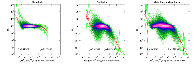
Figure 7: Comparison with the analytical prediction of numerically estimated phase-space density from various contribution of our composite Hernquist halo. The measurement is performed with SPH-AM method using 40 neighbours. The quantity displayed is $f/f_{t}$ as a function of $f_{t}$, where $f$ and $f_{t}$ are the measured and the analytical phase-space distribution functions, respectively. Left panel: main component only. Middle panel: subhaloes, only. In that case the ratio $f/f_{t}$ is computed for each subhalo, individually. Right panel: the full profile, with haloes and subhaloes, while $f_{t}$ is given by the sum of each analytical profile contributing locally.

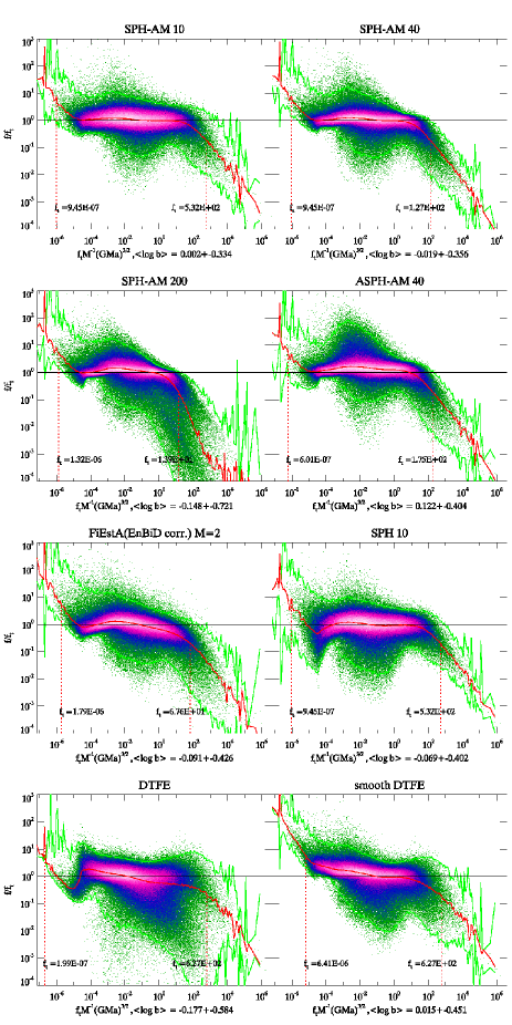
Figure 8: Same as in Figure 4, but the ratio between measured and analytic phase-space distribution function is now shown for our composite Hernquist profile for various smoothing methods as indicated on the top of each panel.

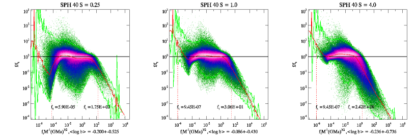
Figure 9: Effect of the choice of the scaling parameter $S_{\rm G}$ between positions and velocities. The ratio $f/f_{t}$ is shown as a function of $f_{t}$, following Figure. 8, but for SPH method with 40 neighbours. From left to right, $S_{\rm G}=0.25h\mbox{ km}~{}\mbox{s}^{-1}~{}\mbox{kpc}^{-1}$, $S_{\rm G}=1h\mbox{ km}~{}\mbox{s}^{-1}~{}\mbox{kpc}^{-1}$, $S_{\rm G}=4.0h\mbox{ km}~{}\mbox{s}^{-1}~{}\mbox{kpc}^{-1}$.

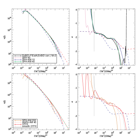
Figure 10: Measurement of $v(f)$ and its logarithmic derivative, following Figure 5, but for the composite Hernquist profile. The blue and red dashed curves correspond to the analytical prediction for the main component and the full halo, respectively. Note that, as discussed in § 3.1, there is a minimum value of $f$ for which we can measure accurately $v(f)$, regardless of the method used, due to the cut-off imposed at radius $r_{\rm cut}$ (dashed vertical line). This is now further complicated by the fact that here, the cut-off is also imposed on the subhaloes, which explains why the measurements tend to slightly overestimate the red dashed curve for $10^{-4}\la f\la 0.1$.

Figure 7 shows the phase-space density estimated by SPH-AM with 40 particles, for the main component, the subhaloes and the full halo. While the theoretical density is a simple sum of all the components contributing locally, it is not exactly the case for the estimated density. By comparing all the plots, one can see that the low-$f$ regime and the high-$f$ regime are dominated by the main component and the subhaloes, respectively. For each component, $f$ presents a large spread in the low density region, $10^{-4}\la f\la 1$, because of the high level of shot noise due to the small number of particles in the edges of substructures, and is underestimated in the high density one. The range of accurate values of $f$ increases with the number of particles in each subhalo. When summing up the subhaloes, as shown in middle panel, this adds up to a significant spread of the scatter plot, obviously much larger than for the main component. In fact, such a spread dominates for the total halo (right panel) and is larger than for a single Hernquist profile with same number of particles (see Figure 4). Because the high phase-space density regime is dominated by subhaloes, the range of recovered values of $f$ is tremendously reduced in that region, and we lose about one order of magnitude for the available high density range compared to the single Hernquist profile. This issue has to be kept in mind when performing the measurements in real $N$-body haloes.

Figure 8, following Figure 4, now compares the various estimators of the phase-space density, and confirms most of our previous findings: the best estimator is SPH-AM with 10 neighbours. It does better than SPH-AM 40 in the high-density regions, because of the lower-level of smoothing, at the cost of a larger spread. The effect is even stronger when performing the comparison with SPH-AM 200, as expected. Again, ASPH-AM with 40 neighbours seems to bring some global estimation bias. EnBiD-FiEstAS with $m_{p}=2$ does not perform any better than SPH-AM since it seems to underestimate $f$ earlier in the high density regime.

Regarding the global scaling, the findings of Figure 4 are confirmed: we obtain the best results by matching the nearest neighbour distance distributions and we measure again (but this coincidence is not generic) $S_{\rm dist}=0.4h\mbox{ km}~{}\mbox{s}^{-1}~{}\mbox{kpc}^{-1}$). The suboptimal nature of the global scaling induces an increase of the amplitude of the scatter below the median, for instance when one compares SPH-AM 10 with SPH 10 on Figure 8. Turning to DTFE in its basic implementation, which stills perform best for low values of $f$ (except for the irregularity already observed in Figure 4), this spread becomes dramatic and strongly asymmetric but can be reduced by using the smoother and more isotropic “spherical” interpolator $f^{\prime}$. Note that, given our factor of five tolerance between measured and exact phase-space density distribution function, DTFE and its smoother version do better than in Figure 4. In fact they now seem to perform slightly better than SPH-AM 10 in the very high-density regime. Indeed, the fraction of overdense particles intervening in the calculation of $S_{\rm dist}$ is much larger: the calculation of $S_{\rm dist}$, corresponding to a compromise between all the particles, is now more adapted to the overdense part of the phase-space distribution function. For the single Hernquist profile, the fraction of particles belonging to the high $f$ part was indeed much smaller. Hence, provided that the proper global scaling between velocities and positions has been set up, DTFE chooses by construction the proper adaptive smoothing range (or the right number of neighbours). However note that the overall shape of the median curve of Figure 8 is not as flat as for SPH-AM, and this is a consequence of the fact that the global scaling is only a compromise that is not locally optimal. In fact, in addition to the small-$f$ irregularity already observed in Figure 4, the high-$f$ plateau in lower-left panel of Figure 8 is somewhat below the thick horizontal line. This follows from the presence of substructures, as discussed above, which does not only induces a strong asymmetry of the spread around the median value: it also biases it to lower values. This is because DTFE uses many neighbours in that regime to perform the interpolation, (about 200 as will be discussed in next section, see Figure 13), which makes it very sensitive to the local anisotropies in the phase-space distribution function. The bias on the high-$f$ plateau is at least partly corrected for by the “spherical” version of DTFE, which is indeed expected to less sensitive to such anisotropies, as illustrated by lower-right panel of Figure 8.

To illustrate in more detail the influence of the choice of the global scaling parameter, $S_{\rm G}$, between velocity space and position space, Figure 9 shows, for our composite profile, how the quality of the measurement of $f$ changes with $S_{\rm G}$ for the SPH method with 40 neighbours (similar trends would be seen for the DTFE method, while adaptive metric methods, e.g. SPH-AM with 40 particles, are by definition totally insensitive to the choice of $S_{\rm G}$). The domain of valid estimates for $f$ considerably depends on the choice of $S_{\rm G}$, as a change by a factor 4 in $S_{\rm G}$ induces a loss by an order of magnitude in the high density range. Note in particular that the shape of the scatter, below the median curve, changes with the actual value of $S_{\rm G}$. For instance, this scatter is reduced in the intermediate range of values for $f$ in the middle panel of Figure 9. This is again a consequence of the fact that the optimal value of $S_{\rm G}$ depends on location in phase-space, in particular on the local distribution of velocities versus positions in the core of substructures, i.e. in the neighbourhood of local density peaks in phase-space.

Following § 3.1, let us finally turn to the measurement of $v(f)$ and its logarithmic derivative, $\alpha(f)$, as illustrated by Figure 10. The analytic calculation of $v(f)$ is similar to § 3.1 except that we now consider each component separately and then combine them straightforwardly. The measurement $v(f)$ itself is performed exactly as explained in § 3.1. The results of Figure 8 are partly confirmed by Figure 10: the best adaptive metric method is again SPH-AM with 10 neighbours. However the best measurements are by far now given by the basic DTFE method (without additional smoothing). Recall that this is due, in part, by the fact that the calculation of $v(f)$ is better behaved for the DTFE method than for other methods: indeed the concept of Eulerian volume is well defined for DTFE, while it remains only approximate with the SPH methods. These methods are optimal when one sits on particles, but get more and more inaccurate when one goes away from the particles. In that sense, Figure 8, which uses a pure Lagrangian point of view, greatly favours the SPH methods, while the measurement of $v(f)$, which is intrinsically an Eulerian quantity, favours more DTFE.

Globally, the measurements in this section suggest that the DTFE method performs rather well, provided that the correct position/velocity scaling is set up. However, the very calculation of the correct value of the scaling factor, $S_{\rm G}$, is not straightforward: in § 3.1, the DTFE method was performing poorly. Even if it is well estimated, this global scaling provides only a compromise, that is not locally optimal.

Finally, let us mention some additional issues about the DTFE method. While exploring various values of $S_{\rm G}$, we found that with larger $S_{\rm G}$, this method starts to generate very large number of Delaunay cells which becomes rapidly impossible to handle computationally. The same happens when we increase the cut-off radius $r_{\rm cut}$: in that case, particles near the border of the catalogue present tremendously large number of Delaunay cells, as they are connected to almost all the other particles. Indeed, it is expected that a high level of local anisotropy increases the number of DTFE neighbours. For all these reasons, we favour the SPH-AM method relative to the DTFE method, even if they seem to perform less well for the measurement of Eulerian quantities such as $v(f)$. Still, if one put aside the problem of position/velocity scaling, the DTFE method provides a local estimate of the optimal number of neighbours, which can help to find the best number of neighbours for the SPH-AM method, as we shall discuss in § 4.1. Finally, while potentially better than the SPH-AM method, the ASPH-AM methods tend to yield a slight overestimation bias for the mid-range of values of $f$, and we did not find a straightforward way to correct for it.

3.3 Haloes from N-body simulations

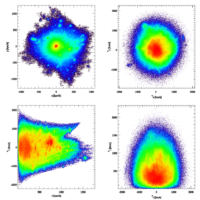
Figure 11: Appearance of our CDM $N$-body halo with 1.8 million particles. This figure can for instance be compared to Figure 6. Upper left panel: $x$–$y$ position space; upper right panel: $v_{x}$–$v_{y}$ velocity space; lower left panel: phase-space diagram, radius $r$–radial velocity $v_{r}$; lower right panel: radial velocity $v_{r}$–tangential velocity $v_{t}$.

We now consider the realistic case of a halo extracted from a Cold Dark Matter (CDM) $N$-body simulation. To do that, we performed a standard CDM simulation with GAGDET2 [Springel 2005] involving $512^{3}$ particles in a periodic cubic box of size $50\ h^{-1}$ Mpc. The choice of the cosmological parameters is matter density $\Omega_{M}=0.3$ and cosmological constant $\Omega_{\Lambda}=0.7$. The linear variance of the density fluctuations in a sphere of radius $8\ h^{-1}$ Mpc is $\sigma_{8}=0.92$ and the Hubble constant fixes $h=0.7$. This is slightly different from recent constrains e.g. provided by WMAP [Spergel et al. 2003] but should be close enough for our purpose. For reference, these cosmological parameters fix the mass of a particle to be $7.7\times 10^{7}M_{\sun}$. Haloes were extracted at present time from this simulation using standard FOF algorithm with linking parameter $b=0.2$. To make the calculations tractable for DTFE, we selected the third most massive halo, which contains about $1.83\times 10^{6}$ particles. Only the linked particles are considered. In the subsequent analyses, calculations are performed in comoving phase-space coordinates instead of physical ones. However, when it comes to phase-space density calculation, the main change when passing from one system of coordinates to the other comes from the effect of the Hubble flow, which has rather insignificant impact on the final results.

Figure 11 displays various projections of the halo, following Figure 6. Here, only one additional complication arises in order to calculate correctly phase-space diagrams: the centre of the halo has to be defined accurately in phase-space. We find this centre through an iterative process, applied to each subspace separately. The first step involves considering the centre as the mean position (velocity) of all the particles. Then, the distance of each particle from this centre is computed and half of the particles are removed by choosing the most distant ones. A new centre is computed from the remaining particles. The process is repeated again as long as there are more than 100 particles left.

As noted earlier, the velocity subspace (upper panels of Fig. 11) is relatively featureless. Figure 11 is in fact very similar to Figure 6, except for the lower-left panel which displays more complex structures. In particular, in addition to the vertical “fingers”, one can notice some elongated structures that correspond to non trivial filamentation of phase-space built up by the dynamics, e.g. tidal tails (see for instance Peirani & Pacheco 2007).

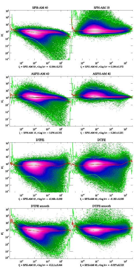
Figure 12: Phase-space density estimation for our CDM $N$-body halo with $1.8$ million particles. The left and right columns correspond to the SPH-AM method with 10 and 40 neighbours, respectively, for the theoretical phase-space density, $f_{t}$. From top to bottom, the smoothing method considered is (a) the SPH-AM method with 40 neighbours on the left panel and SPH-AM with 10 neighbours on the right panel, (b) the ASPH-AM with 40 neighbours on the left and ASPH-AM with 10 neighbours on the right panel, (d) the basic DTFE method and (e) DTFE method with spherical smoothing.

In this more realistic framework, we cannot rely on an analytic expression of the reference $f_{t}$ to perform plots similar to Figures 4 and 8. However since the SPH-AM methods have our preference, we shall now use them as references. This is illustrated by Figure 12, which shows the ratio $f/f_{t}$ as a function of $f_{t}$ for various smoothing methods; $f_{t}$ is given this time by the SPH-AM methods with 10 and 40 neighbours, for respectively the left and right columns. Note that $f$ and $f_{t}$ are measured for each particle individually to perform these scatter plots. To fix the global scaling position/velocity parameter for the DTFE implementations, we use a coincidence scaling of the peak distance distribution given by $S_{\rm G}=S_{\rm dist}=0.38h\mbox{ km}~{}\mbox{s}^{-1}~{}\mbox{Mpc}^{-1}$.

Figure 12 confirms qualitatively the results found for the single and the composite Hernquist profiles. In particular, the SPH-AM methods with 40 neighbours underestimates high phase-space densities compared to the SPH-AM 10 method. In the upper left panel of Figure 12, there is also a tail below the median curve, which arises because the measured $f$ is significantly biased toward lower values nearby local phase-space density peaks corresponding to each substructure, as explained in previous section; this local bias is more prominent for the SPH-AM 40 than SPH-AM 10 method, and consequently the median curve of the upper left panel is slightly below unity, except for low-$f$. This bias can be reduced with adaptive smoothing, as shown in the second row of Figure 12 with the ASPH-AM 40 method. But recall that this is achieved at a price of a slight uncontrollable positive bias, here in underdense phase-space regions. The DTFE method seems to behave well overall, with a positive bias in underdense phase-space regions when implementing its smoother version. However, our appreciation is again skewed by the somewhat loose factor of five tolerance. In fact, DTFE in its simpler implementation seems to globally underestimate the phase-space density distribution function, except in the very-low and in the very-high density regimes. Again, this is due to the contribution from substructures, which is now more significant given the larger effective number of neighbours used by DTFE and its high sensitivity to the choice of the local scaling, $S_{\rm L}$. The effect of the tail below the median value is therefore now more significant than for the upper left panel, and it is reduced, as well as the bias of the median curve in intermediate values of $f$, by the spherical implementation (lowest panels of Figure 12). Hence Figure 12 globally confirms the findings of Figure 8. Note that we do not observe any irregularity in the low-$f$ regime as in Figure 8, because the cut-off of the halo is performed in a much smoother way.

4 Additional insights

Although the Delaunay tessellation cannot easily address the problem of the position/velocity scaling, because of it self adaptive nature, it still provides some insight about the local neighbourhood, in particular about the optimal number of neighbours that should be used in SPH methods. In § 4.1, we analyse in details the neighbour distribution provided by the Delaunay tessellation. This will help us to better understand the results found in the previous sections and to further justify our preference for the SPH-AM estimator with a number of neighbours ranging from 10 to 40.

The analyses of § 3 show that the entropy method implemented in EnBiD provides a very good approximation of the local scaling to apply between positions and velocities. In § 4.2, we investigate how this scaling depends on the environment, and in particular on the value of $f$. This will allow us to better understand to choice of the global scaling.

4.1 Smoothing range and local neighbourhood

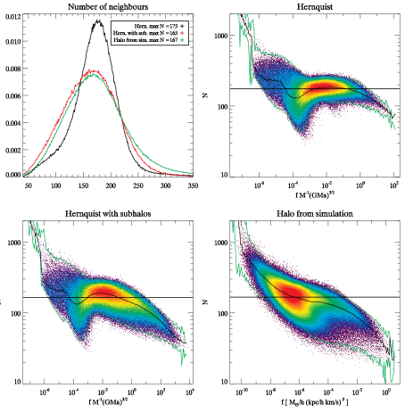
Figure 13: Number of neighbours $N$ found by the Delaunay tessellation for the three profiles considered in this paper. Top left panel: the probability distribution function, $P(N)$, for a particle of having $N$ neighbours. Top right panel: $N$ is shown as a function of the theoretical phase-space density, $f_{t}$, for our single Hernquist profile. The horizontal line corresponds to the mean value of $N$, while the smooth black curve gives the median as a function of $f_{t}$. Bottom left panel: $N$ is shown as a function of the theoretical phase-space density, for our composite Hernquist profile. Bottom right panel: $N$ is shown as a function of the phase-space density measured in our dark matter simulated halo.

In Figure 13, we study the distribution of the number of neighbours built by the Delaunay structure as a function of phase-space density, for the single Hernquist profile of § 3.1 (upper right panel), the composite Hernquist profile of § 3.2 (lower left panel) and the $N$-body halo of § 3.3 (lower right panel). The upper left panel shows, for each instance, the overall distribution function of the number of neighbours.

As expected, the average number of neighbours is approximately the same in the three cases: $\langle N\rangle=175$, 165 and 167, for the Hernquist profile, the composite Hernquist profile and the $N$-body halo, respectively. The presence of substructures widens the overall distribution of values of $N$, as shown by the green and the red curves in upper left panel of Figure 13, as compared to the black one. In the three cases considered, the typical number of neighbours decreases with increasing phase-space density, following three regimes:

1. particles near the edges: at the edges of the catalogue, where $f$ is very small, $N$ is very large, of the order of 1000 for the Hernquist cases up to nearly 10 000 for the $N$-body halo. It then decreases rapidly, while particles are getting away from the edges to reach the next regime, (ii). Note that $N$ being large is not a consequence of $f$ being small, but follows from the fact that the phase-space distribution function presents an overall positive curvature and is highly anisotropic because of the edges.

2. The plateau at intermediate values of $f$, far from the edges and from the main distribution of local maxima: in this quiescent regime, we have $N\sim\langle N\rangle$, where $\langle N\rangle$ is the typical number of expected Delaunay neighbours just as quoted above. Note that there is a slight difference between the Hernquist profiles and the $N$-body halo, in particular a lower bump at $f\simeq 10^{-4.5}$ in upper right and lower left panels, that corresponds to the transition between regime (i) and regime (ii), and which does not appear for the $N$-body halo. This is probably due to the brutal cut-off imposed at radius $r_{\rm cut}$ as mentioned in § 3.1, which can affect the neighbour distribution in a non trivial manner up to $f\simeq 10^{-4.41}$ for the single Hernquist profile and the main component of the composite Hernquist profile.

3. The high density regime, dominated by the regions nearby local maxima: the number of neighbours decreases again rapidly because $f$ now presents an increasingly overall negative curvature when one reaches the densest regions, which makes $N$ smaller; we measure it to be as small as 30 in the presence of substructures (which dominate large values of $f$, as noticed in § 3.2), while it remains close to 100 in the single Hernquist profile.

Intuitively these numbers suggest that, when turning to SPH methods, the number of neighbours used to perform the interpolation should depend on the environment. In particular, in the “quiescent” regime, i.e. far from the edges and from the peaks, we should take around 200 neighbours to perform the measurements. However, such a large number of neighbours is not optimal near the peaks: the DTFE algorithm suggests a value of $N$ of the order of a few tens for sampling best the core of substructures, which is fully confirmed by the analyses of our previous sections. Furthermore we noticed that these values of $N=10$ and $N=40$ are still appropriate in the quiescent regime: only the signal to noise ratio –the spread due to local Poisson noise around the local average value– is changed. Taking a value of $N$ as large as 200 provides too much smoothing and biases the results in overdense regions. Moreover it also induces non trivial diffusing mixing effects. The larger the number of neighbours, the more sensitive the determination of $f$ to local anisotropies.

Such local anisotropies (and local curvature properties) can be captured better –at least partly– by anisotropic SPH smoothing (see the discussion in § 2.3 and Figure 2), but at a risk of some potential slight positive biases, as argued previously. Since SPH methods in their usual implementation are not self adaptive in terms of their number of neighbours, we think that the best choice for $N$ is a value ranging from 10 to 40, because such a choice offers a good compromise for all the dynamic range. Note that this also confirms the findings of S06. There is still the problem of what happens near the edges, but these can sometimes be extended sufficiently far away to avoid contamination of the measurements in the region of interest. What really influences the results are abrupt changes of local curvature: while the DTFE method captures them optimally, SPH method does it only approximately, and of course, does it best when the number of neighbours remains small, at the expense of a slightly worse local signal to noise ratio.

Note, however, that this discussion is again biased by the fact that SPH uses a Lagrangian point of view, i.e. it sits on the centre of each particle to measure locally the phase-space distribution function. An Eulerian point of view, that would require to measure $f$ in an arbitrary point of space (see, e.g., Colombi, Chodorowski & Teyssier 2007), would probably impose a slightly larger number of neighbours for SPH methods to give sensible results.

Note finally that the findings of Figure 13 are of course sensitive to the choice of the velocity/position scaling $S_{\rm G}$ which is taken here to be equal to $S_{\rm dist}$ as discussed in previous sections. Indeed, the value of $S_{\rm G}$ influences the properties of the local curvature of the distribution function (or the matrix of its second derivatives), so we expect the low-$f$ and particularly the high-$f$ regimes to be affected by the chosen $S_{\rm G}$ (Fig. 9).

4.2 On the EnBiD position-velocity scaling

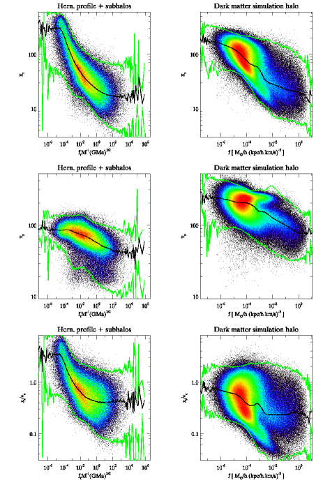
Figure 14: Local position-velocity scaling given by the EnBiD algorithm as a function of phase-space density. The left and right columns correspond to the composite Hernquist profile of § 3.2 and the simulated halo of § 3.3, respectively. From top to bottom, the position subspace scaling, $s_{x}$, the velocity subspace scaling, $s_{v}$, and the ratio $S_{\rm L}=s_{x}/s_{v}$. In the left panels, the phase-space density is the theoretical one. In the right panels, it is measured in the sample using SPH-AM with 40 neighbours.

In the EnBiD algorithm, one gets for each particle a hyperbox of size $2s_{x}$ in position subspace and of size $2s_{v}$ in velocity subspace. Figure 14 shows the measured value of $s_{x}$, $s_{v}$ and $S_{\rm L}=s_{x}/s_{v}$ as functions of $f$, for our composite Hernquist profile (left columns) and our $N$-body halo (right columns). The global behaviour of the quantities $s_{x}(f)$ and $s_{v}(f)$ as decreasing functions of $f$ (the median curves in the four upper panels of Figure 14) is expected, as increasing phase-space density corresponds to a smaller size for the local hypercube. Due to the more concentrated extension of substructures in position rather than in velocity space, the corresponding decrease is more significant for $s_{x}(f)$ –by an order of magnitude– than for $s_{v}(f)$ –by about a factor 2. As a result, the ratio $S_{\rm L}=s_{x}/s_{v}$ changes from about $1.3-0.7$ in the low-$f$ regime to $0.4-0.3$ in the high-$f$ regime (see the median curve in two lower panels of Figure 14).

When examining in more details the scatter plots on the right panels of Figure 14, we note a bimodal structure: the cloud of points splits into two fingers at high $f$. The shorter and denser finger corresponds to the main part of the halo, while the other corresponds to the contribution of substructures, which are more concentrated in phase-space than the central part of the halo. This last statement can be easily checked by looking at the upper right panel of Figure 18. The main part of the halo is globally relaxed so its concentration in velocity space does not depend significantly on the value of $f$ (the upper horizontal finger in the middle right panel of Figure 14), while its position density behaves approximately like a power-law (lower roughly straight and diagonal finger in the upper right panel of Figure 14). On the other hand, substructures are tidally disrupted and lose particles while they spiral into the halo: they represent a population of objects at various dynamical states, different from the dynamical state of the main part of the halo. This explains the bimodality observed in right panels of Figure 14. It would however go beyond the scope of this paper to fully explain the details of this bimodality. It is indeed difficult to disentangle the effect of the local change of substructure phase-space/velocity subspace/position subspace profile due to tidal deformation, in particular to a mass loss, from the statistical averaging carried over the population of all the substructures.

Note that, even though the prescription used to create the Hernquist composite profile is dynamically unrealistic, there still should be a bimodal effect in this experiment, because the substructures present a population of objects at various “dynamical states”, different from the main component, owing to the fact that they are less massive. However, in addition to having unrealistic individual profiles, the contribution of substructures was purposely exaggerated: they are more massive than those of the simulated halo. Consequently, the bimodality is much less obvious on the left panels of Figure 14 than on the right panels. Of course, this difference only partly accounts for this finding, as tidal stripping changes the individual profiles of subhaloes [Stoehr 2006] and also produces tidal tails that contribute in a non trivial way to filamentation of phase-space.

The bimodal nature of the distribution of the ratio $s_{x}/s_{v}$ has a dramatic impact on methods which rely on a global scaling between positions and velocities prior to the measurement of the distribution function. Furthermore, apart from that problem and the large scatter of this ratio (of about one order of magnitude), its median value changes with $f$, as mentioned earlier. Note however the plateau reached at high values of $f$, a regime dominated by substructures, where $s_{x}/s_{v}\simeq 0.3$. The global average of the ratio is equal to 0.7 and 0.5 for the Hernquist composite profile and the simulated halo, respectively, while $S_{\rm dist}=0.4$ and 0.38. It is important to notice that the values of $S_{\rm dist}$ are thus close to the high-$f$ plateau, showing that high values of $f$ are expected to be calculated with nearly optimal scaling parameter using our peak matching of the distance distribution.

5 Revisiting a proxy to phase-space estimation

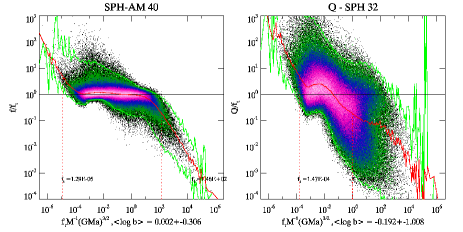
Figure 15: True phase-space density estimator (left panel) versus the proxy $Q=\rho/\sigma^{3}$ in our Hernquist composite profile. The ratio $f/f_{t}$ is shown as a function of $f_{t}$, where $f$ and $f_{t}$ are the measured and the exact phase-space densities, respectively. To generate the left panel, we used SPH-AM with 40 neighbours. To measure the function $Q({\bf x})$ on the right panel, we use a standard SPH interpolation in position space with 32 neighbours to estimate locally $\rho({\bf x})$ and measure the velocity dispersion $\sigma^{2}({\bf x})$ with the same position space kernel.

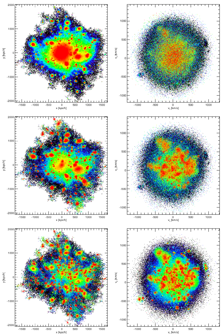
Figure 16: Appearance of the CDM $N$-body haloes in position space (left panels) and in velocity space (right panels), with different colour codings. The pictures are computed in 3 steps as follows: (i) division of space into three dimensional equally spaced grid with $N=400$ divisions across each $x,y,z$ axes, (ii) calculation of the mean density ($\rho$,$f$,$Q$) of all particles inside each cell and (iii) projection of this density on the $x-y$ plane by taking in each $z$ column the cell with the highest density. Only $40\%$ of the central cells along the $z$ axis are used for the last step. The first, second and third rows correspond respectively to a colour coding with the projected density $\rho$, with the parameter $Q=\rho/\sigma^{3}$ and with phase-space density $f$. To enhance the contrasts, the equalisation of the histograms of the logarithm of $\rho$, $Q$ and $f$ was implemented.

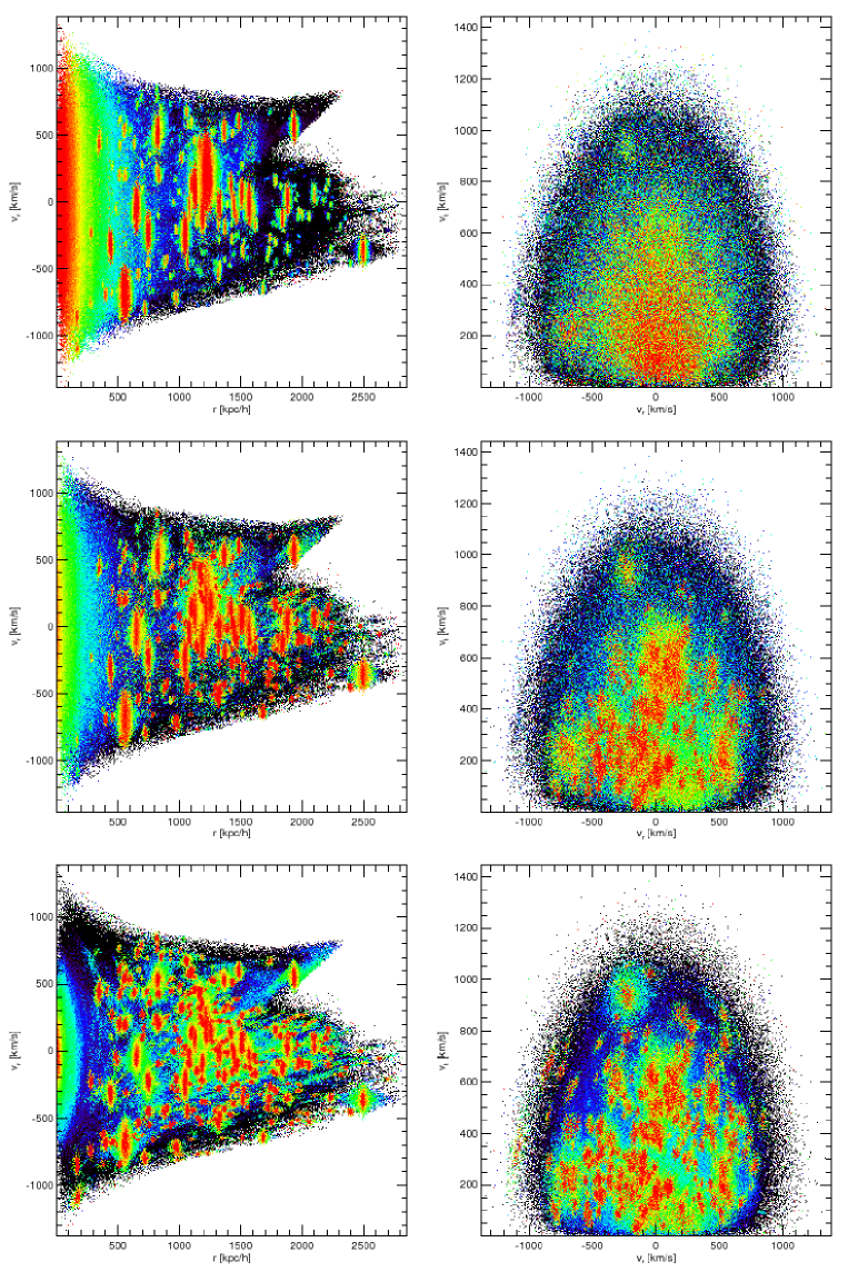
Figure 17: Appearance of the CDM $N$-body haloes in radius/radial velocity space (left panels) and in radial/tangential velocity space (right panels), using the same colour coding rules as in Figure 16, namely using $\rho$, $Q$ and $f$ for the first, second and third rows, respectively.

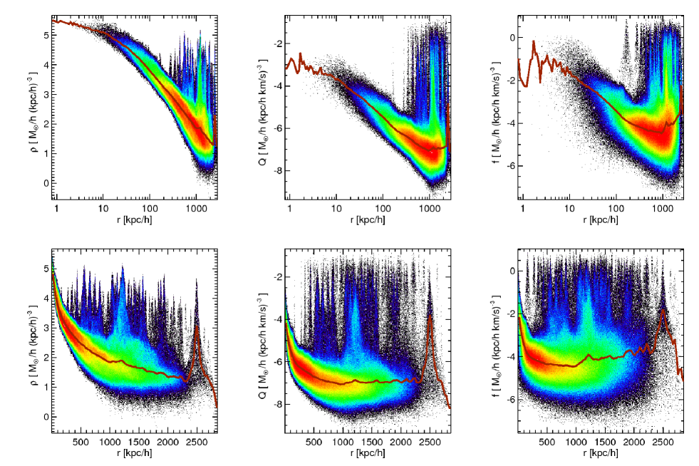
Figure 18: Measured densities, from left to right, $\rho$, $Q$ and $f$, as functions of distance $r$ from the halo centre in our CDM $N$-body halo. For the top and bottom rows, the density is represented as a function of $\log r$ and $r$, respectively, while the thick line is calculated by taking local median.

Prior to the existence of 6D phase-space density estimators, an approximation of the phase-space density was proposed, which involves only the measurement of quantities in position space rather than in full 6D phase-space (see for instance, Taylor & Navarro, 2001):

$$Q({\bf x}) = \rho({\bf x})/\sigma^{3}({\bf x}),$$ (27)

$$= {3}^{3/2}\frac{\left[{\int f(\mathbf{x},\mathbf{v}){\rm d}^{3}v}\right]^{5/2}}{\left[\int{v^{2}f(\mathbf{x},\mathbf{v}){\rm d}^{3}v}\right]^{3/2}},$$ (28)

where $\rho({\bf x})$ is the local projected density and $\sigma^{3}({\bf x})$ is the local one dimensional velocity dispersion defined as $\sigma=\sqrt{(\sigma_{x}^{2}+\sigma_{y}^{2}+\sigma_{z}^{2})/3}$. The function $Q({\bf x})$ has been widely used in the literature as a proxy of the true “phase-space” distribution function [Taylor & Navarro 2001, Rasia et al. 2005, Austin et al. 2005, Peirani & de Freitas Pacheco 2007, Diemand, Kuhlen & Madau 2006]. It is often defined in a spherically average way, $Q(r)=\rho(r)/\sigma^{3}(r)$. For instance, Taylor & Navarro (2001) found that $Q(r)\propto r^{-\alpha}$ with $\alpha=1.875$, in good agreement with the secondary infall model [Bertschinger 1985].

To relate $Q(x)$ to the true phase-space density in a more intuitive way than equation (28), we can assume that $f(\mathbf{x},\mathbf{v})$ factorises as follows:

$$f(\mathbf{x},\mathbf{v})=\frac{\rho({\bf x})}{(2\pi)^{3/2}\sigma^{3}({\bf x})}\exp\left\{-\frac{[{\bf v}-{\bf v}_{0}({\bf x})]^{2}}{2\sigma^{2}({\bf x})}\right\},$$ (29)

where proper normalisations were set up directly. Hence,

$$f(\mathbf{x},\mathbf{v})=Q({\bf x})\frac{1}{(2\pi)^{3/2}}\exp\left\{-\frac{[{\bf v}-{\bf v}_{0}({\bf x})]^{2}}{2\sigma^{2}({\bf x})}\right\}.$$ (30)

In particular, $Q({\bf x})=f[{\bf x},{\bf v}_{0}({\bf x})](2\pi)^{3/2}$. We see that, within a normalisation factor, function $Q({\bf x})$ is representative of the true phase-space distribution function where it matters, i.e. in the neighbourhood of local maxima in velocity space. Of course, this argument is valid only if at fixed ${\bf x}={\bf x}_{0}$, the function $g({\bf v})=f({\bf x}_{0},{\bf v})$ presents only one local maximum in ${\bf v}$ space. If this condition is verified, we could expect the function $Q({\bf x})$ to represent a fair estimate of the true phase-space distribution function near the local maxima in phase-space, which correspond to substructures. However this is not strictly true since substructures a embedded in the background of the main component of the halo: $\sigma({\bf x})$ is not the local velocity dispersion of the substructure but rather the local velocity dispersion of the diffuse component, which is much larger. We therefore expect $Q({\bf x})$ to underestimate the true distribution function in substructures, corresponding to the high $f$ regime, which is dominated by these clumps. On the other hand, when considering the main component of the halo, which dominates the low $f$ regime, we expect $Q({\bf x})$ to overestimate the true distribution function, as, $f({\bf x},{\bf v})<f({\bf x},{\bf v}_{0})$ for ${\bf v}\neq{\bf v}_{0}$ in equation (29). These arguments rely on the very simple modeling given by equation (29), but they are confirmed by Figure 15, which compares the measured function $Q({\bf x})$ to the exact solution for the Hernquist composite profile studied in § 3.2. Similar trends are observed for the simulated halo, not shown here.

Clearly, the function $Q$ corresponds to a serious shortcoming when compared to the realistic phase-space estimators studied in this paper. However it seems to capture the main features of the distribution function, as illustrated by Figures 16 and 17. These figures compare, in various subspaces, the structures obtained when colour is coded by projected density $\rho({\bf x})$, using the parameter $Q({\bf x})$, and by phase-space density. They are supplemented with Figure 18, which shows $\rho$, $Q$ and $f$ as functions of distance $r$ from the halo centre. Note interestingly that, both for the 6D estimator and its proxy $Q$, the maximum value of phase-space density in substructures seems to be approximately the same for all the substructures (and larger than at the centre of the halo). This property is quite useful as it makes substructure detection quite easy with simple friend-of-friend algorithm, as proposed by Diemand et al. (2006). These authors do not use the true phase-space distribution function but the function $Q$ to carry the detection.

While pure projected density codes provide much less information than phase-space density ones, the $Q({\bf x})$ function seems to capture the most important features of phase-space, and in particular subhaloes. However, the true phase-space density provides additional crucial information, in particular subtle phase-space structures such as the fine filaments observed in the $(r,v_{r})$ diagram, some of which being at the origin of caustics, others corresponding to tidal tails. In a forthcoming work, we shall discuss the detection and analysis of substructures in phase-space. We shall see that analysis of substructures in phase-space can be used to infer powerful properties on the dynamical history of dark matter haloes.

6 Summary

We devoted this paper to the study of six-dimensional phase-space density estimators in $N$-body samples. We considered several methods used in the literature to estimate phase-space density that differ from each other (i) in the way the tessellation of space is performed, and (ii) in the way local interpolation is performed. Concerning point (i), we consider two kind of tessellations: the Delaunay tessellation (DTFE) proposed by Arad et al. (2004) through the SHESHDEL algorithm and the hierarchical decomposition of phase-space using binary tree technique as proposed by Ascasibar & Binney (2004) through the FiEstAS algorithm, later improved by Sharma & Steinmetz (2006) with the EnBiD implementation. In the (ii) class, we consider two ways of estimating the phase-space density for the DTFE method, one based on the direct estimation of the local Delaunay cells volumes, and a more isotropic, smoother version of it. For the binary tree method, we consider the hypercubical cell smoothing proposed in FiEstAS and the standard SPH smoothing (but in 6D instead of 3D) using an Epanechikov kernel as advocated by S06. We also test an anisotropic SPH method (ASPH).

In all these methods, a crucial problem is to set properly the local metric frame to relate position and velocities, which basically sets a scaling factor between the position and the velocity subspace. While the binary tree methods can be optimised locally both through their refinement and through the definition of such a system of coordinates — using a Shannon entropy criterion, as advocated by S06 and implemented through the EnBiD algorithm, a global metric must also be defined for the DTFE method, prior to the construction of the tessellation network.

In order to automatically specify a global metric, we presented two methods which yield similar results. The first one involves simple dynamical arguments based on the properties of NFW profiles. The second method involves measuring the nearest neighbour distance distributions in position and in velocity subspace and finding the scaling factor between position and velocities for which the positions of the peak of these two distributions match each other.

To summarise, we tested the following implementations:

1. the DTFE algorithm and a smoother, more isotropic version of it. Both of them require the definition of a global metric;

2. the FiEstAS binary tree method with EnBiD improvement;

3. SPH methods (a) with EnBiD improvement and (b) without it. We denote case (a) by SPH-AM, i.e. SPH with adaptive metric, in opposition to case (b) that we simply denote by SPH; which requires a global metric setting;

4. Adaptive SPH methods with adaptive metric (ASPH-AM).

To test the various algorithm in details, we used three halo models:

(a)

A Hernquist isotropic profile with $5\times 10^{5}$ particles. In that case, analytical estimates are available for the phase-space distribution function.

(b)

A composite Hernquist halo, built from a main component with $2.5\times 10^{5}$ particles, and a set of substructures amounting to $2.5\times 10^{5}$ particles. In that more realistic case, there is also an exact expression for the phase-space distribution function.

(c)

A $N$-body halo with 1.8 millions particles extracted from a standard CDM simulation.

The main results of our analyses are the following:

• Because they are local and adaptive, the SPH-AM methods provide the best estimators for the phase-space density, when using a moderate number of neighbours, ranging from 10 to 40 in order to perform the interpolation.

• While DTFE estimators are in principle better than SPH estimators when one measures Eulerian quantities (not centred on the particle positions), they generally perform poorly in phase-space because they rely on a global metric setup. A dynamically consistent measurement of the phase-space distribution function requires that the scaling between positions and velocity be locally adaptive. The best compromise, without supplementary assumption on the dynamical history of the system, is achieved by enforcing local isotropy in phase-space: this is achieved in practice by the Shannon entropy criterion used in EnBiD. Note finally a last weakness of DTFE methods: they are extremely costly from a computational point of view compared to SPH-AM, both in terms of computer time and memory.

• While the optimal number of neighbours should typically be around 200 as suggested by DTFE, we find, using also DTFE, that it should be around a few tens near high density peaks, which justifies the low value we suggest to use for the SPH-AM method: such a number increases noise to signal ratio, but allows us to probe better high phase-space density peaks.

• By analysing the properties of the local metric proposed by EnBiD, we find that the distance distribution matching method provides a global scaling between positions and velocities which probes well the high density regions of phase-space, which are dominated by substructures. We also find that the actual “optimal” local scaling presents a bimodal distribution, made from the contribution of the main component of the halo, roughly in equilibrium, and the contribution of the substructures, which are tidally disrupted while they spiral in within the halo. This bimodality and the corresponding large scatter of about one order of magnitude on the local scaling parameter between positions and velocities has a dramatic impact on the performance on methods relying on global metric setting, such as DTFE.

• the ASPH-AM methods do not bring much improvement over the SPH-AM implementation. They can potentially improve phase-space estimation in high density regions, but at the cost of a slight systematic overestimation bias in the moderate density regime.

Note that most of our estimators are Lagrangian in nature,i.e. they estimate phase-space density at particles positions: in that sense they favour the SPH approach relatively to the DTFE approach. One has to keep in mind that DTFE tessellates accurately all space, while the SPH smoothing becomes increasingly suboptimal while departing from the particles. In particular, we found that an Eulerian quantity such as $v(f)$ was still best measured by DTFE, despite the problem of the suboptimal position/velocity scaling.

Alternative routes to phase-space density estimation could involve using the angle-action canonical variables which match the closest spherical fit to a given halo. Indeed, the topology of the underlying tori would provide a natural setting in which to coarse grain the distribution.

References

- [Alard & Colombi 2005] Alard C., Colombi S., 2005, MNRAS, 359, 123
- [Arad et al. 2004] Arad I., Dekel A., Klypin A., 2004, MNRAS, 353, 15
- [Ascasibar & Binney 2004] Ascasibar Y., Binney J. 2005, MNRAS, 356, 872
- [Austin et al. 2005] Austin C., Williams L., Barnes E., Babul A., Dalcanton J., 2005, ApJ, 634, 756
- [Bernardeau & van de Weygart 1996] Bernardeau F., van de Weygaert R., 1996, MNRAS, 279, 693
- [Bertschinger 1985] Bertschinger E., 1985, ApJS, 58, 39
- [Binney & Tremaine 2008] Binney J., Tremaine S., 2008, Galactic dynamics, Princeton Univ. Press, Princeton, NJ
- [Colombi, Chodorowski & Teyssier 2007] Colombi S., Chodorowski M., Teyssier R., MNRAS, 375, 348
- [Diemand, Kuhlen & Madau 2006] Diemand J., Kuhlen M., Madau P., 2006, ApJ, 649, 1
- [Hayashi et al. 2007] Hayashi E., Navarro J. F., Springel, V., 2007, MNRAS, 377, 50
- [Huchra & Geller 1982] Huchra J.P., Geller M.J., 1982, ApJ 257, 423
- [Hernquist 1990] Hernquist L., 1990, ApJ 356, 359
- [Jing & Suto 2002] Jing Y. P., Suto Y., 2002, ApJ, 574, 538
- [Moore et al. 1998] Moore B., Governato F., Quinn T., Stadel J., Lake G., 1998, ApJ, 499, L5
- [Moore et al. 1999] Moore B., Ghigna S., Governato F., Lake G., Quinn T., Stadel J., Tozzi P., 1999, ApJ, 524, L19
- [Navarro, Frenk and White 1997] Navarro J.F., Frenk C.S., White S. D. M., 1997, ApJ, 490, 493
- [Peirani & de Freitas Pacheco 2007] Peirani, S., de Freitas Pacheco, J. A., 2007, astro-ph/0701292
- [Pelupessy et al. 2003] Pelupessy F. I., Schaap W. E., van de Weygaert R., 2003, A&A 403, 389
- [Rasia et al. 2005] Rasia E., Tormen G., Moscardini L., 2004, MNRAS, 351, 237
- [Romano-Diaz & van de Weygaert 2007] Romano-Diaz E., van de Weygaert R., 2007, MNRAS, 382, 2
- [Schaap & van de Weygaert 2003] Schaap W. E., van de Weygaert R. 2003, Statistical Challenges in Astronomy, 483
- [Schneider, 2006] Schneider P., 2006, Extragalactic Astronomy and Cosmology: An Introduction, Springer
- [Sharma & Steinmetz 2006] Sharma S., Steinmetz M., 2006, MNRAS 373, 1293
- [Spergel et al. 2003] Spergel D.N., Verde L., Peiris H.V., et al., 2003. ApJS 148, 175
- [Springel 2005] Springel V., 2005, MNRAS, 364, 1105
- [Springel et al. 2001] Springel V., White S. D. M., Tormen G., Kauffmann G., 2001, MNRAS, 328, 726
- [Stadel 2001] Stadel J.G., PhD thesis, University of Washington, 2001
- [Stoehr 2006] Stoehr F., 2006, MNRAS, 365, 147
- [Taylor & Navarro 2001] Taylor J. E., Navarro J. F., 2001, ApJ, 563, 483
- [Tremaine et al. 1986] Tremaine S., Henon M., Lynden-Bell D., 1986, MNRAS, 219, 285
- [Vogelsberger et al. 2008] Vogelsberger M., White S.D.M., Helmi A., Springel V., 2008, MNRAS, 385, 236
- [Weygaert & Shaap 2007] van de Weygaert R., Schaap W., 2007, astro-ph/0708.1441v1