Semilinear response for the heating rate
of cold atoms in vibrating traps

Abstract

The calculation of the heating rate of cold atoms in vibrating traps requires a theory that goes beyond the Kubo linear response formulation. If a strong “quantum chaos” assumption does not hold, the analysis of transitions shows similarities with a percolation problem in energy space. We show how the texture and the sparsity of the perturbation matrix, as determined by the geometry of the system, dictate the result. An improved sparse random matrix model is introduced: it captures the essential ingredients of the problem, and leads to a generalized variable range hopping picture.

The rate of energy absorption by particles that are confined by vibrating walls was of interest in past studies of nuclear friction [1, 2, 3], where it leads to the damping of the wall motion. More recently it has become of interest in the context of cold atoms physics. In a series of experiments [4, 5, 6] with “atom-optics billiards” some surprising predictions [7] based on linear response theory (LRT) have been verified.

In the present study we consider the case where the billiard is fully chaotic [a] but with nearly integrable shape (Fig.1). We explain that in such circumstances LRT is not applicable (unless the driving is extremely weak such that relaxation dominates). Rather, the analysis that is relevant to the typical experimental conditions should go beyond LRT, and involve a “resistor network” picture of transitions in energy space, somewhat similar to a percolation problem. Consequently we predict that the rate of energy absorption would be suppressed by orders of magnitude, and provide some analytical estimates which are supported by a numerical calculation.

We assume that an experimentalist has control over the position ($R$) of a wall element that confines the motion of cold atoms in an optical trap. We consider below the effect of low frequency noisy (non periodic) driving. This means that $R$ is not strictly constant in time, either because of drifts [8] that cannot be eliminated in realistic circumstances, or else deliberately as a way to probe the dynamics of the atoms inside the trap [9]. We assume the usual Markovian picture of FGR transitions between energy levels, which is applicable in typical circumstances (see e.g. [10]). These transitions lead to diffusion in the energy space. If the atomic cloud is characterized by a temperature $T$, then the diffusion in energy would lead to heating with the rate $\dot{E}=D/T$ [b] and hence to an increase in the temperature of the cloud.

Naively one expects to observe an LRT behavior. That means to have $D\propto[\mbox{RMS}(\dot{R})]^{2}$, and more specifically to have a linear relation between the diffusion coefficient and the power spectrum of the driving:

$$D\ \ \equiv\ \ G\times\mbox{RMS}(\dot{R})^{2}\ \ =\ \ \int_{0}^{\infty}\tilde{C}(\omega)\tilde{S}(\omega)d\omega$$ (1)

Here $\tilde{S}(\omega)$ is the power spectrum of $\dot{R}$, and $\tilde{C}(\omega)$ is related to the susceptibility of the system. From the experimentalist’s point of view the second equality in Eq.(1) can be regarded as providing a practical definition for $\tilde{C}(\omega)$, if the response is indeed linear.

We shall explain in this paper that the applicability of LRT in our problem is very limited, namely LRT would lead to wrong predictions in typical experimental circumstances. Rather we are going to use a more refined theory, which we call semi-linear response theory (SLRT) [11, 12], in order to determine $D$. The theory is called SLRT because on the one hand the power spectrum ${\tilde{S}(\omega)\mapsto\lambda\tilde{S}(\omega)}$ leads to ${D\mapsto\lambda D}$, but on the other hand ${\tilde{S}(\omega)\mapsto\tilde{S}_{1}(\omega)+\tilde{S}_{2}(\omega)}$ does not lead to ${D\mapsto D_{1}+D_{2}}$. This semi-linearity can be tested in an experiment in order to distinguish it from linear response. Accordingly, in SLRT the spectral function $\tilde{C}(\omega)$ of Eq.(1) becomes ill defined, while the coefficient $G$ is still physically meaningful, and can be measured in an actual experiment.

If we assume small driving amplitude the Hamiltonian matrix can be written as ${\mathcal{H}=\{E_{n}\}+f(t)\{V_{nm}\}}$, where

$$V_{nm}\ \ =\ \ \Big{\langle}n\Big{|}\frac{d\mathcal{H}}{dR}\Big{|}m\Big{\rangle}$$ (2)

is the perturbation matrix. More than 50 years ago Wigner had proposed to regard the perturbation matrix of a complex system as a random matrix (RMT) whose elements are taken from a Gaussian distribution. Later Bohigas had conjectured that the same philosophy applies to quantized chaotic systems. For such matrices the validity of LRT can be established on the basis of the FGR picture, and the expression for $G$ is the Kubo formula $G_{\mbox{\tiny LRT}}=\pi\varrho_{\mbox{\tiny E}}\langle\langle|V_{nm}|^{2}\rangle\rangle_{a}$ where ${\langle\langle x\rangle\rangle_{a}=\langle x\rangle}$ is the algebraic average over the near diagonal matrix elements [c], and $\varrho_{\mbox{\tiny E}}$ is the density of states (DOS). In contrast to that, using the Pauli master equation [10] with FGR transition rates between levels, the SLRT analysis leads to

$$G_{\mbox{\tiny SLRT}}\ \ =\ \ \pi\varrho_{\mbox{\tiny E}}\,\langle\langle|V_{nm}|^{2}\rangle\rangle$$ (3)

where the “average” $\langle\langle x\rangle\rangle$ is defined as in Ref.[11, 12] via a resistor-network calculation [13]. (For mathematical details see “the SLRT calculation” paragraph below).

Within the RMT framework an element $x$ of $|V_{nm}|^{2}$ is regarded as a random variable, and the histogram of all $x$ values is used in order to define an appropriate ensemble. For the sake of later discussion we define, besides the algebraic average ${\langle\langle x\rangle\rangle_{a}}$ also the harmonic average as ${\langle\langle x\rangle\rangle_{h}=[\langle 1/x\rangle]^{-1}}$ and the geometric average as ${\langle\langle x\rangle\rangle_{g}=\exp[\langle\ln x\rangle]}$. The result of the resistor network calculation is labeled as $\langle\langle x\rangle\rangle$ (without subscript).

Our interest is in the circumstances where the strong “quantum chaos” assumption of Wigner fails. This would be the case if the distribution of $x$ is wide in log scale. If $x$ has (say) a log-normal distribution, then it means that the typical value of $x$ is much smaller compared with the algebraic average. This means that the perturbation matrix $V_{nm}$ is effectively sparse (a lot of vanishingly small elements). We can characterize the sparsity by the parameter ${q=\langle\langle x\rangle\rangle_{g}/\langle\langle x\rangle\rangle_{a}}$. We are going to explain that for typical experimental conditions we might encounter sparse matrices for which ${q\ll 1}$. Then the energy spreading process is similar to a percolation in energy space, and the SLRT formula Eq.(3) replaces the Kubo formula.

1 Outline

In what follow we present our model system, analyze it within the framework of SLRT, and then introduce an RMT model with log-normal distributed elements, that captures the essential ingredients of the problem. We show that a generalized resistor network analysis for the transitions in energy space leads to a generalized Variable Range Hopping (VRH) picture (the standard VRH picture has been introduced by Mott in [14] and later refined by [15] using the resistor network perspective of [13]). Our RMT based analytical estimates are verified against numerical calculation. Finally we discuss the experimental aspect, and in particular define the physical circumstances in which SLRT rather than LRT applies. These two theories give results that can differ by orders of magnitude.

2 Modeling

Consider a strictly rectangular billiard whose eigenstates are labeled by ${\bm{n}=(n_{x},n_{y})}$. The perturbation due to the movement of the ‘vertical’ wall does not couple states that have different mode index $n_{y}$. Due to this selection rule the perturbation matrix is sparse. If we deform slightly the potential (Fig.1a), or introduce a bump (Fig.1b), then states with different mode index are mixed. Consequently the numerous zero elements become finite but still very tiny in magnitude, which means a very wide size distribution featuring a small fraction of large elements. Similar considerations apply for the circular cavity of Fig.1c, where an off-center scatterer couples radial and angular motion, and which is more suitable for a real experiment (but less convenient for numerical analysis).

Typically the perturbation matrix is not only sparse but also textured. This means (see Fig.2) that there are stripes where the matrix elements are larger, and bottlenecks where they are all small. The emergence of texture (i.e. non-random arrangement of the sparse large elements along the diagonals) is most obvious if we consider the geometry of Fig.1d, where we have a divided cavity with a small weakly connected chamber where the driving is applied. If the chamber were disconnected, then only chamber states with energies $E_{r}$ would be coupled by the driving. But due to the connecting corridor there is mixing of bulk states with chamber states within energy stripes around $E_{r}$. The coupling between two cavity states $E_{n}$ and $E_{m}$ is very small outside of the $E_{r}$ stripes. Consequently the near diagonal elements of $V_{nm}$ have wide variation, and hence a wide $\log(x)$ distribution.

Coming back to the geometries of Fig.1abc, it is somewhat important in the analysis to distinguish between smooth deformation that couples only nearby modes, and diffractive deformation that mix all the modes simultaneously: Recalling that different modes have different DOS, and that low-DOS modes are sparse within the high-DOS modes, we expect a more prominent manifestation of the texture in the case of a smooth deformation of a cavity that has a large aspect ratio. We later confirm this expectation in the numerical analysis.

3 The SLRT calculation

As in the standard derivation of the Kubo formula, also within the framework of SLRT [11, 12], the leading mechanism for absorption is assumed to be FGR transitions. The FGR transition rate is proportional to the squared matrix elements $|V_{nm}|^{2}$, and to the power spectrum at the frequency ${\omega=E_{n}{-}E_{m}}$. It is convenient to define the normalized spectral function $\tilde{F}(\omega)$, such that

$$\tilde{S}(\omega)\ \ \equiv\ \ \mbox{RMS}(\dot{R})^{2}\times\tilde{F}(\omega)$$ (4)

Contrary to the naive expectation the theory does not lead to the Kubo formula. This is because the rate of absorption depends crucially on the possibility to make connected sequences of transitions. It is implied that both the texture and the sparsity of the $|V_{nm}|^{2}$ matrix play a major role in the calculation of $G$. Consequently SLRT leads to Eq.(3), where ${\langle\langle...\rangle\rangle}$ is defined using a resistor network calculation. Namely, the energy levels are regarded as the nodes of a resistor network, and the FGR transition rates as the bonds that connect different nodes. Following [12] the inverse resistance of a bond is defined as

$$\mathsf{g}_{nm}\ \ \equiv\ \ 2\varrho_{\mbox{\tiny E}}^{-3}\ \frac{|V_{nm}|^{2}}{(E_{n}{-}E_{m})^{2}}\ \tilde{F}(E_{m}{-}E_{n})$$ (5)

and ${\langle\langle|V_{nm}|^{2}\rangle\rangle}$ is defined as the inverse resistivity of the network. It is a simple exercise to verify that if all the matrix elements are the same, say ${|V_{nm}|^{2}=c}$, then ${\langle\langle|V_{nm}|^{2}\rangle\rangle=c}$ too. But if the matrix is sparse or textured then typically

$$\langle\langle|V_{nm}|^{2}\rangle\rangle_{\mbox{\tiny h}}\ll\langle\langle|V_{nm}|^{2}\rangle\rangle\ll\langle\langle|V_{nm}|^{2}\rangle\rangle_{\mbox{\tiny a}}$$ (6)

In the case of sparse matrices this is a mathematically strict inequality, and we can use a generalized VRH scheme which we describe below in order to get an estimate for $\langle\langle x\rangle\rangle$. If the element-size distribution of $\log(x)$ is not too stretched a reasonable approximation is ${\langle\langle x\rangle\rangle\approx\langle\langle x\rangle\rangle_{\mbox{\tiny g}}}$, simply because the geometric mean is the typical (median) value for the size of the elements. However, if $|V_{nm}|^{2}$ has either a very stretched element-size distribution, or if it has texture, then our VRH analysis below show that the geometric average becomes merely an improved lower bound for the actual result.

4 Analysis

We consider a particle of mass $\mathsf{M}$ in a two dimensional box of length $L_{x}$ and width $L_{y}$, such that ${0<x<L_{x}}$ and ${0<y<L_{y}}$. See Fig.1b. With the driving the length of the box becomes ${R=L_{x}+f(t)}$. The Hamiltonian is

$$\mathcal{H}=\mbox{diag}\{E_{\bm{n}}\}+u\{U_{\bm{n}\bm{m}}\}+f(t)\{V_{\bm{n}\bm{m}}\}$$ (7)

where $\bm{n}=(n_{x},n_{y})$ is a composite index that labels the energy levels $E_{\bm{n}}$ of a particle in a rectangular box of size ${L_{x}\times L_{y}}$. The deformation is described by a normalized Gaussian potential $U(x,y)$ of width $(\sigma_{x},\sigma_{y})$ positioned at the central region of the box. Its matrix elements are $U_{\bm{n}\bm{m}}$, and it is multiplied in the Hamiltonian by a parameter $u$ which signifies the strength of the deformation. Note that the limit ${\sigma\rightarrow 0}$ is well defined and corresponds to an “s-scatterer”. The perturbation matrix due to the $f(t)$ displacement of the wall is

$$V_{\bm{n}\bm{m}}\ \ =\ \ -\delta_{n_{y},m_{y}}\times\frac{\pi^{2}}{\mathsf{M}L_{x}^{3}}n_{x}m_{x}$$ (8)

The power spectrum of $\dot{f}$ is assumed to be constant within the frequency range $|\omega|<\omega_{c}$ and zero otherwise. This means that ${\tilde{F}(\omega)=1}$ up to this cutoff frequency. We have also considered (not presented) an exponential line shape ${\tilde{F}(\omega)=\exp(-|\omega/\omega_{c}|)}$, leading to qualitatively similar results. After diagonalization of ${\{E_{\bm{n}}\}+u\{U_{\bm{n}\bm{m}}\}}$ the Hamiltonian takes the form

$$\mathcal{H}=\mbox{diag}\{E_{n}\}+f(t)\{V_{nm}\}$$ (9)

where $n$ (not bold) is a running index that counts the energies in ascending order. The DOS remains essentially the same as for ${u=0}$, namely,

$$\varrho_{\mbox{\tiny E}}\ \ =\ \ \frac{1}{2\pi}\mathsf{M}L_{x}L_{y}$$ (10)

The perturbation matrix $|V_{nm}|^{2}$ is sparse and textured (see Fig.2). First we discuss the sparsity, and the effect of the texture will be addressed later on.

Considering first zero deformation ($u=0$) it follows from Eq.(8) that the non-zero elements of the perturbation matrix are ${|V_{nm}|^{2}\approx|\mathsf{M}v_{\mbox{\tiny E}}^{2}/L_{x}|^{2}}$, where ${v_{\mbox{\tiny E}}=\sqrt{2E/\mathsf{M}}}$. The algebraic average of the near diagonal elements equals this value (of the large size elements) multiplied by their percentage $p_{0}$. To evaluate $p_{0}$ let us consider an energy window $dE$. The number of near-diagonal elements $V_{nm}$ within the stripe ${|E_{n_{x},n_{y}}{-}E_{m_{x},m_{y}}|<d\varepsilon}$ is ${\varrho_{\mbox{\tiny E}}^{2}dEd\varepsilon}$. It is a straightforward exercise to find out that the the number of non-zero elements (i.e. with ${n_{y}{=}m_{y}}$) is the same number multiplied by ${p_{0}=[2\pi\mathsf{M}v_{\mbox{\tiny E}}L_{y}]^{-1}}$. Consequently

$$\langle\langle|V_{nm}|^{2}\rangle\rangle_{a}\approx\left[\frac{1}{2\pi\mathsf{M}v_{\mbox{\tiny E}}L_{y}}\right]\left|\frac{\mathsf{M}v_{\mbox{\tiny E}}^{2}}{L_{x}}\right|^{2}=\frac{\mathsf{M}v_{\mbox{\tiny E}}^{3}}{2\pi L_{y}L_{x}^{2}}$$ (11)

Somewhat surprisingly this result turns out to be the same (disregarding an order unity numerical prefactor) as for a strongly chaotic cavity (see Eq.(I3) of Ref.[3]), as if there is no sparsity issue. This implies that irrespective of the deformation $u$, the LRT Kubo result is identical to the 2D version of the wall formula (see Sec.7 of Ref.[3]):

$$G_{\mbox{\tiny LRT}}\ \ =\ \ \frac{4}{3\pi}\frac{\mathsf{M}^{2}v_{\mbox{\tiny E}}^{3}}{L_{x}}$$ (12)

Our interest below is not in $G_{\mbox{\tiny LRT}}$ but in $G_{\mbox{\tiny SLRT}}$, which can differ by many orders of magnitudes. For sufficiently small $u$ the large size matrix elements are not affected, and therefore the algebraic average stays the same. But in the SLRT calculation we care about the small size matrix elements, that are zero if ${u=0}$. Due to the first-order mixing of the levels, the typical overlap ${|\langle\bm{m}|n\rangle|}$ between perturbed and unperturbed states is ${|uU_{\bf{n}\bf{m}}/(E_{\bm{n}}{-}E_{\bm{m}})|}$. The typical size of a small $V_{nm}$ element is the multiplication of this overlap (evaluated for nearby levels) by the size of a non-zero $V_{\bm{n}\bm{m}}$ element. Consequently the small size matrix elements are proportional to $u^{2}$. The geometric average simply equals their typical size, leading to

$$\langle\langle|V_{nm}|^{2}\rangle\rangle_{g}\approx\left(\frac{\mathsf{M}^{2}v_{\mbox{\tiny E}}^{2}}{2\pi L_{x}}\right)^{2}\,\mbox{e}^{-2\mathsf{M}^{2}v_{\mbox{\tiny E}}^{2}(\sigma_{x}^{2}+\sigma_{y}^{2})}\ u^{2}$$ (13)

Motivated by the discussion below Eq.(6) a crude estimate for the SLRT result is ${G_{\mbox{\tiny SLRT}}\approx q\times G_{\mbox{\tiny LRT}}}$, where for small deformation

$$q\ \ =\ \ \frac{\langle\langle|V_{nm}|^{2}\rangle\rangle_{g}}{\langle\langle|V_{nm}|^{2}\rangle\rangle_{a}}\ \ \propto\ \ u^{2}\ \ \ \ \ \ \ \mbox{see Eqs.(\ref{e21},\ref{e22})}$$ (14)

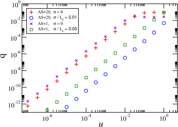
Figure 4: The sparsity parameter $q$ is plotted versus the strength $u$ of the deformation potential for cavities with aspect ratios ${AS=1}$ and ${AS=20}$. We see that for large aspect ratio $q$ has some sensitivity to $\sigma$. As explained in the text $G_{\mbox{\tiny SLRT}}/G_{\mbox{\tiny LRT}}$ is correlated with $q$, but for large aspect ratio it is even more sensitive to $\sigma$ due to the emergence of textures whose presence is not reflected by the value of $q$.

It follows from the above (and see Fig.4) that for small deformations $q\ll 1$, and consequently we expect ${G_{\mbox{\tiny SLRT}}\ll G_{\mbox{\tiny LRT}}}$. This should be contrasted with the case of strongly deformed box for which all the elements are of the same order of magnitude and $q$ becomes of order unity. Our next task is to further improve the SLRT estimate using a proper resistor network calculation [d].

5 RMT modeling

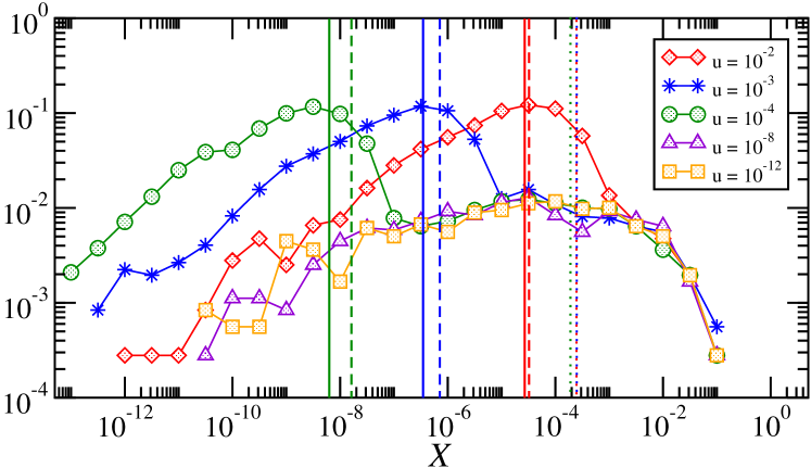
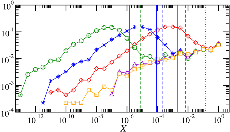
Figure 3: Histograms of matrix elements for different values of $u$ for ${AS=1}$ (upper) and ${AS=20}$ (lower). Here we assume a ${\sigma=0}$ scatterer. The vertical lines for ${u=10^{-2},10^{-3},10^{-4}}$ indicate the $\langle\langle x\rangle\rangle$ obtained from the LRT algebraic average (3 dotted lines that are barely resolved), from the SLRT resistor network calculation (solid lines), and from the untextured calculation (dashed lines). The geometric mean approximately coincides with the peaks, and underestimates the SLRT value for the larger $AS$ where the sparsity is much larger.

The $|V_{nm}|^{2}$ matrix looks like a random matrix with some distribution for the size of the elements (see Fig.3). It might also possess some non-trivial texture which we ignore within the RMT framework. The RMT perspective allows us to derive a quantitative theory for $G$ using a generalized VRH estimate. Let us demonstrate the procedure in the case of an homogeneous (neither banded nor textured) random matrix with log-normal distributed elements. The mean and the variance of $\ln(x)$ are trivially related to geometric and the algebraic averages. Namely, ${\langle\ln(x)\rangle=\ln{\langle\langle x\rangle\rangle_{\mbox{\tiny g}}}}$ and ${\mbox{Var}(x)=-2\ln(q)}$. Given a hopping range ${|E_{m}-E_{n}|\leq\omega}$ we can look for the typical matrix element $x_{\omega}$ for connected sequences of transitions, which we find by solving the equation ${\varrho_{\mbox{\tiny E}}\omega\mbox{F}(x_{\omega})\sim 1}$, where $\mbox{F}(x)$ is the probability to find a matrix element larger than $x$. This gives

$$x_{\omega}\ \ \approx\ \ \langle\langle x\rangle\rangle_{\mbox{\tiny g}}\exp\left[2\sqrt{-\ln q^{\alpha}}\right]$$ (15)

where $\alpha=\ln(\varrho_{\mbox{\tiny E}}\omega_{c})$. From this equation we deduce the following: For $q{\lesssim}1$, meaning that the distribution is not too wide, $x_{\omega}\approx\langle\langle x\rangle\rangle_{\mbox{\tiny g}}$ as anticipated. But as the matrix gets more sparse (${q\ll 1}$), the result deviates from the geometric average, the latter becoming merely a lower bound.

The generalized VRH estimate is based on optimization of the integral $\int x_{\omega}\,\tilde{F}(\omega)\,d\omega$. For the rectangular $\tilde{F}(\omega)$ which has been assumed below Eq.(8) this optimization is trivial and gives $\approx x_{\omega_{c}}$, leading to

$$G_{\mbox{\tiny SLRT}}\ \ =\ \ q\ \exp\left[2\sqrt{-\ln q^{\alpha}}\right]\times G_{\mbox{\tiny LRT}}$$ (16)

where $G_{\mbox{\tiny LRT}}$ is given by Eq.(12) and $q$ is given by Eq.(14). We have also tested the standard VRH that assumes an exponential $\tilde{F}(\omega)$ (not presented).

6 Numerical results

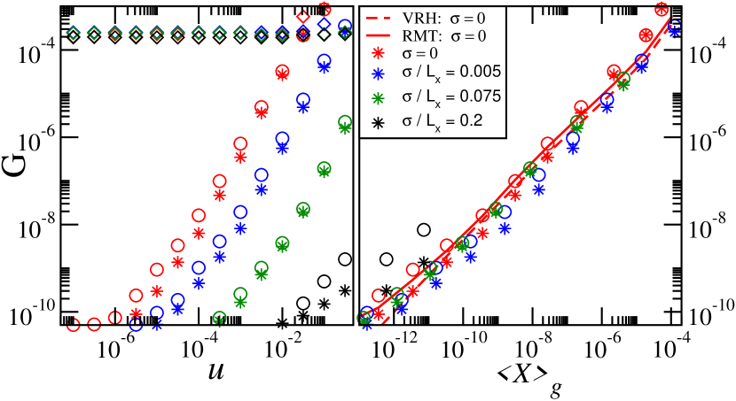
Figure 5: Left panel: The scaled $\tilde{G}\equiv\langle\langle x\rangle\rangle$ in the LRT and in the SLRT case as a function of $u$ for ${AS=1}$ and different smoothness of the deformation. The stars are for the physical matrices, while the circles are for their untextured versions (see text). The diamonds are for the LRT case. Right panel: The SLRT result ${\langle\langle x\rangle\rangle}$ versus the geometric average ${\langle\langle x\rangle\rangle_{\mbox{\tiny g}}}$. These are compared with RMT based results, and with the associated analytical estimate of Eq.(16). We see the the agreement is very good.

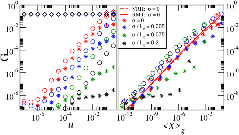
Figure 6: The same set of plots as in Fig.5 but for ${AS=20}$. In the right panel we clearly see the departure of the physical result from the untextured and RMT results, and hence from the analytical estimate of Eq.(16).

The analytical estimates in Eqs.(11,13) are supported by the histograms of Fig.3. For each choice of the parameters ${(AS,\sigma,u)}$ we calculate the algebraic, and the geometric and the SLRT resistor network averages of $\{|V_{nm}|^{2}\}$. See Fig.5 and Fig.6. We also compare the actual results for $G_{\mbox{\tiny SLRT}}$ with those that were obtained from a log-normal RMT ensembles with the same algebraic and geometric averages as that of the physical matrix [e]. As further discussed in the next paragraph one concludes that the agreement of the physical results with the associated VRH estimate Eq.(16) is very good whenever the perturbation matrix is not textured, which is in fact the typical case for non-extreme aspect ratios.

In order to figure out whether the result is fully determined by the distribution of the elements or else texture is important we repeat the calculation for untextured versions of the same matrices. The untextured version of a matrix is obtained by performing a random permutation of its elements along the diagonals. This procedure affects neither the bandprofile nor the $\{|V_{nm}|^{2}\}$ distribution, but merely removes the texture. In Fig.5 we see that the physical results cannot be distinguished from the untextured results, and hence are in agreement with the RMT and with the associated VRH estimate. On the other hand, in Fig.6, which is for large aspect ratio, we see that the physical results deviate significantly from the untextured result. As the width of the Gaussian potential becomes larger (smoother deformation), the texture becomes more important. These observation are in complete agreement with the expectations that were discussed in the modeling section.

7 Experiment

As in [4, 5, 6] a collection of $N{\sim}10^{6}$ atoms, say ${}^{85}Rb$ atoms (${\mathsf{M}=1.4\times 10^{-25}kg}$), are laser cooled to low temperature of ${T\sim 10\mu K}$, such that the the typical thermal velocity is ${v_{\mbox{\tiny E}}\sim 0.05m/s}$. The atoms are trapped in an optical billiard whose blue-detuned light walls confine the atoms by repulsive optical dipole potential. The motion of the atoms is limited to the billiard plane by a strong perpendicular optical standing wave. The thickness of the billiard walls (${\sim 10\mu m}$) is much smaller than its linear size (${L\sim 200\mu m}$). The 2D mean level spacing is ${\Delta=\varrho_{\mbox{\tiny E}}^{-1}\sim 2.5\times 10^{-34}J}$, which is ${2.4Hz}$. One or more of the billiard walls can be vibrated with several kHz frequency by modulating the laser intensity. The dimensionless spectral bandwidth of this driving can be set as say ${\omega_{c}/\Delta\sim 1000}$, with an amplitude ${\sim 10\mu m}$, such that ${\dot{R}\sim 0.015m/s}$. The temperature of the trapped atoms can then be measured as a function of time by the time-of-flight method. The LRT estimate ${G_{\mbox{\tiny LRT}}\sim 1.3\times 10^{-51}Js/m^{2}}$ would lead to heating rate ${\dot{E}\sim 2\times 10^{-27}J/s}$ which is ${\sim 0.15mK/s}$. Considering (say) the geometry of Fig.1c, the deformation ($u$) is achieved either by introducing an off center optical “spot”, or by deforming slightly the optical walls (such precise control on the geometry has been demonstrated in previous experiments). Having control over $u$ we can have ${q\sim 10^{-5}}$ that would imply factor $100$ suppression, i.e. an estimated heating rate of few ${\mu K/sec}$. Such heating rate can be accurately measured, yielding high sensitivity to the energy diffusion process studied here.

8 SLRT vs LRT

Typically the environment introduces in the dynamics an incoherent relaxation effect. If the relaxation rate is strong compared with the rate of the externally driven transitions, then the issue of having “connected sequences of transitions” becomes irrelevant, and the SLRT slowdown of the absorption is not expected. In the latter case LRT rather than SLRT is applicable. It follows that for finite relaxation rate there is a crossover from LRT to SLRT behavior as a function of the intensity of the driving. In cold atom experiments the relaxation effect can be controlled, and typically it is negligible. Hence SLRT rather than LRT behavior should be expected. This implies, as discussed above, a much smaller absorption rate. Furthermore, as discussed in the introduction, one can verify experimentally the signature of SLRT: namely, the effect of adding independent driving sources is expected to be non-linear with respect to their spectral content.

9 Conclusions

In this work we have introduced a theory for the calculation of the heating rate of cold atoms in vibrating traps. This theory, that treats the diffusion in energy space as a resistor network problem, is required if the cavity is not strongly chaotic and if the relaxation effect is small. The SLRT result, unlike the LRT (Kubo) result is extremely sensitive to the sparsity and the textures that characterize the perturbation matrix of the driving source. For typical geometries the ratio between them is determined by the sparsity parameter $q$ as in Eq. (16), and hence is roughly proportional to the deformation ($u^{2}$) of the confining potential. If the cavity has a large aspect ratio, and the deformation of the confining potential is smooth, then the emerging textures in the perturbation matrix of the driving source become important, and then the actual SLRT result becomes even smaller.

By controlling the density of the trapped atoms, or their collisional cross section (e.g. via the Feshbach resonance) the atomic collision rate can be tuned by many orders of magnitude. Their effect on the dynamics can thus be made either negligible (as assumed above) or significant, thereby serving as an alternative (but formally similar) mechanism for weak breakdown of integrability. It follows that heating rate experiments can be used not only to probe the deformation ($u$) of the confining potential, but also to probe the interactions between the atoms.

Acknowledgments. – This research was supported by a grant from the USA-Israel Binational Science Foundation (BSF).

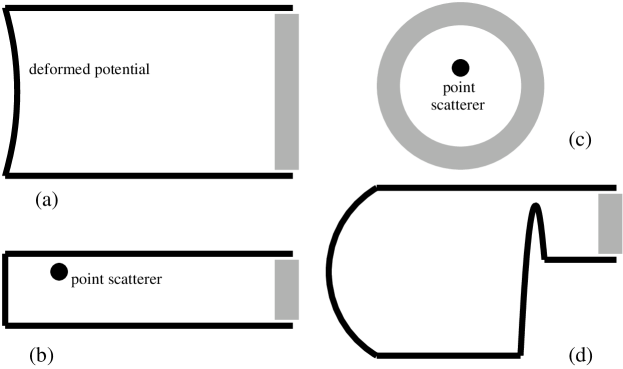
Figure 1: Model systems: The atoms are held by a potential that may consist of static walls (solid lines), a vibrating wall (shaded lines), and bumps (thick points). The numerics has been done for (b) with a Gaussian bump. We work with two different aspect ratios. For the aspect ratio $AS=20$ we take $L_{x}=200$ and $L_{y}=10$. For the aspect ratio $AS=1$ we take $L_{x}=40$ and $L_{y}=40$. The position of the Gaussian bump was randomly chosen within the region ${[0.4,0.6]L_{x}\times[0.4,0.6]L_{y}}$. The width of the Gaussian is $\sigma_{x}=\sigma_{y}=\sigma$. We have assumed noisy driving with $\omega_{c}=7\Delta$, where $\Delta=1/\varrho_{\mbox{\tiny E}}$ is the mean level spacing, and the units were such that $\mathsf{M}=1$.

Figure 2: Image of the perturbation matrix $|V_{nm}|^{2}$ due to a wall displacement of a rectangular-like cavity that has an aspect ratio ${AS=20}$. The potential floor is deformed due to the presence of a ${\sigma{=}0}$ scatterer with ${u=10^{-4}}$ (see text). The matrix is both sparse and textured. Lower inset: untextured matrix - the elements along each diagonal are randomly permuted. Upper inset: non-sparse matrix with the same band profile - each element is generated independently from a normal distribution.

References

- [1] J. Blocki, Y. Boneh, J.R. Nix, J. Randrup, M. Robel, A.J. Sierk and W.J. Swiatecki, Ann. Phys. 113, 330 (1978).
- [2] S.E. Koonin, R.L. Hatch and J. Randrup, Nucl. Phys. A 283, 87 (1977). S.E. Koonin and J. Randrup, Nucl. Phys. A 289, 475 (1977).
- [3] D. Cohen, Annals of Physics 283, 175 (2000); cond-mat/9902168.
- [4] N. Friedman, A. Kaplan, D. Carasso, and N. Davidson, Phys. Rev. Lett. 86, 1518 (2001).
- [5] A. Kaplan, N. Friedman, M. F. Andersen, and N. Davidson, Phys. Rev. Lett. 87, 274101 (2001).
- [6] M. Andersen, A. Kaplan, T. Grunzweig and N. Davidson, Phys. Rev. Lett. 97, 104102 (2006).
- [7] A. Barnett, D. Cohen and E.J. Heller, Phys. Rev. Lett. 85, 1412 (2000); J. Phys. A 34, 413 (2001).
- [8] T. A. Savard, L. M. Ohara and J. E. Thomas, Phys. Rev. A 56, R1095 (1997).
- [9] S. Friebel, C. D’Andrea, J. Walz, M. Weitz, and T. W. Hansch, Phys. Rev. A 57, R20 (1998).
- [10] W.H. Louisell, Quantum Statistical Properties of Radiation, (Wiley, London, 1973).
- [11] D. Cohen, T. Kottos and H. Schanz, J. Phys. A 39, 11755 (2006). M. Wilkinson, B. Mehlig, D. Cohen, Europhysics Letters 75, 709 (2006).
- [12] S. Bandopadhyay, Y. Etzioni and D. Cohen, Europhysics Letters 76, 739 (2006). A. Stotland, R. Budoyo, T. Peer, T. Kottos and D. Cohen, J. Phys. A 41, 262001 (FTC) (2008).
- [13] A. Miller and E. Abrahams, Phys. Rev. 120, 745 (1960).
- [14] N.F. Mott, Phil. Mag. 22, 7 (1970).
- [15] V. Ambegaokar, B. Halperin, J.S. Langer, Phys. Rev. B 4, 2612 (1971). M. Pollak, J. Non-Cryst. Solids 11, 1 (1972).
- [a] Our interest is in systems that are classically chaotic. This means exponential sensitivity to change in initial conditions, without having mixed phase space.
- [b] For a more general version of , that does not assume a Boltzmann-like distribution with a well defined temperature, see section IV of Ref.[3].
- [c] The average is taken over all the elements within the energy window of interest as determined by the preparation temperature. The weight of in this average is determined by the spectral function as .
- [d] For a very small , an optional route that bypass the resistor network calculation, is to analyze the slow () transitions between noise-broadened energy levels.
- [e] Since for the log-normal distribution the median equals the geometric average, we used the median in the definition of for the sake of the numerical stability.