Large-$\boldmath{N}$ phase transitions in the spectrum of products of complex matrices

Abstract:

It is shown that the simplest multiplicative random complex matrix model generalizes the large-$N$ phase structure found in the unitary case: A perturbative regime is joined to a nonperturbative regime at a point of nonanalyticity.

1 Introduction

Recent numerical work provides evidence that Wilson loops in $SU(N)$ gauge theory in two, three and four dimensions exhibit an infinite-$N$ phase transition: Dilated from a small size to a large one, the eigenvalue distribution of the untraced Wilson loop unitary matrix expands from a small arc to the entire unit circle [1, 2]. This transition, which was discovered by Durhuus and Olesen [3], is in the universality class of a random multiplicative ensemble of unitary matrices [4]. In the following, we will relax the unitarity constraint and focus on a multiplicative random complex matrix model introduced and solved in [5].

2 Basic random complex matrix model

We define a sequence of $n$ independent and identically distributed $N\times N$ matrices

$$M_{j}=\exp\left(\epsilon C_{j}\right)\>,\quad j=1,\ldots,n$$ (1)

with normalized Gaussian probability distribution

$$P(C)d\mu(C)=e^{-N\operatorname{tr}C^{\dagger}C}\prod_{1\leq i,j\leq N}\frac{N}{\pi}\underbrace{d\mu(C_{ij})}_{d\operatorname{Re}(C_{ij})\>d\operatorname{Im}(C_{ij})}$$ (2)

which is invariant individually under $C_{j}\to C^{*}_{j},-C_{j}$ and $C_{j}\to U_{j}^{\dagger}C_{j}U_{j},~{}U_{j}\in U(N)$. We do not restrict the trace of $C_{j}$ here since it turns out that requiring $\det M_{j}=1$ has no effect on the saddle-point analysis in the large-$N$ limit. We are interested in the distribution of the product

$$W_{n}=\prod_{j=1}^{n}M_{j}$$ (3)

in the limit $n\to\infty,~{}\epsilon\to 0$ with the parameter $t=\epsilon^{2}n$ held fixed. $t>0$ can be interpreted as a diffusion time. This model is almost identical to that of [5].

To derive a closed formula for the entire distribution of $W$ for general $N$ is difficult; however, similarly to the unitary model, partial information about the distribution of eigenvalues can be obtained from the averages of characteristic polynomials. In the following, averages over all $C_{j}$ are denoted by $\langle\dots\rangle$. $\langle\det(z-W_{n})\rangle$ carries no information, since

$$\langle\det(z-W_{n})\rangle=(z-1)^{N}\>.$$ (4)

The first non-trivial case is

$$Q(z,z^{*})=\langle|\det(z-W_{n})|^{2}\rangle\>.$$ (5)

Applying large-$N$ factorization to $Q$ (i.e., assuming that the average of the product can be replaced by the product of the averages) would result in holomorphic factorization,

$$Q(z,z^{*})\rightarrow\langle\det(z-W_{n})\rangle\langle\det(z-W_{n})^{*}\rangle=|z-1|^{2N}\>,$$ (6)

and all eigenvalues seem to have to be unity. This factorization is expected to hold only in two distinct regions: inside a circle around zero with radius $\rho<1$ and outside a circle of radius $\rho^{-1}>1$. Therefore, the surface eigenvalue density is restricted to the annulus $\rho<|z|<\rho^{-1}$. The aim of the following is to calculate $Q$ as a function of $t$. We shall find that the domain of eigenvalues becomes multiply connected at a critical $t=t_{c}$, in agreement with [5].

3 Saddle-point analysis

The first step in the procedure is to disentangle the non-abelian product of matrices defining $W_{n}$. To this end, we introduce $2nN$ pairs of Grassmann variables $\left\{\bar{\psi}_{j},\psi_{j},\bar{\chi}_{j},\chi_{j}\right\}_{j=1,\ldots,n}$ and find

$$|\det(z-W_{n})|^{2}=\int\prod_{j=1}^{n}[d\bar{\psi}_{j}d\psi_{j}d\bar{\chi}_{j}d\chi_{j}]e^{\sum_{j=1}^{n}(e^{\sigma}\bar{\psi}_{j}\psi_{j}+e^{\sigma^{*}}\bar{\chi}_{j}\chi_{j})}e^{-\sum_{j=1}^{n}(\bar{\psi}_{j}M_{j}\psi_{j+1}+\bar{\chi}_{j}M^{\dagger}_{j}\chi_{j-1})}$$ (7)

with $z=e^{n\sigma}$ and the convention that $\psi_{n+1}\equiv\psi_{1}$, etc.

Now, the integrals over the matrices $C_{j}$ factorize and can be done explicitly to sufficient accuracy in $\epsilon$. The following equalities ought to be understood in the sense that they hold up to terms which vanish as $n\to\infty$, $\epsilon\to 0$ at $t=\epsilon^{2}n$ fixed. An expansion of $M=\exp(\epsilon C)$ to linear order in $\epsilon$ is sufficient because the next term does not contribute,

$$\langle e^{-\bar{\psi}M\psi^{\prime}-\bar{\chi}M^{\dagger}\chi^{\prime}}\rangle=e^{-\bar{\psi}\psi^{\prime}-\bar{\chi}\chi^{\prime}-\frac{\epsilon^{2}}{N}\bar{\psi}\chi^{\prime}\bar{\chi}\psi^{\prime}}\>.$$ (8)

Introducing scalar complex bosonic multipliers $\zeta_{j}$, $j=1,\ldots,n$ allows for a separation of the quartic Grassmann terms into bilinears,

$$e^{-\frac{\epsilon^{2}}{N}\bar{\psi}\chi^{\prime}\bar{\chi}\psi^{\prime}}=\frac{N}{\pi}\int d\mu(\zeta)e^{-N|\zeta|^{2}}e^{-\epsilon(\zeta\bar{\psi}\chi^{\prime}-\zeta^{*}\bar{\chi}\psi^{\prime})}\>,$$ (9)

where the integration measure is $d\mu(\zeta)=d\operatorname{Re}\zeta\>d\operatorname{Im}\zeta$. After shifting some indices of Grassmann variables, this leads to

$$Q(z,z^{\ast}) =\left(\frac{N}{\pi}\right)^{n}\int\prod_{j=1}^{n}[d\bar{\psi}_{j}d\psi_{j}d\bar{\chi}_{j}d\chi_{j}d\mu(\zeta_{j})]e^{-N\sum_{j=1}^{n}|\zeta_{j}|^{2}}e^{-\sum_{j=1}^{n}(\bar{\psi}_{j}\psi_{j}+\bar{\chi}_{j}\chi_{j})}$$

$$\quad\times e^{\sum_{j=1}^{n}(e^{\sigma}\bar{\psi}_{j}\psi_{j-1}+e^{\sigma^{*}}\bar{\chi}_{j}\chi_{j+1})}e^{-\epsilon\sum_{j=1}^{n}(\zeta_{j}\bar{\psi}_{j}\chi_{j}-\zeta^{*}_{j}\bar{\chi}_{j}\psi_{j})}\>.$$ (10)

As a result, averages over complex matrices $C_{j}$ are replaced by averages over complex numbers $\zeta_{j}$. Carrying out the integrals over the Grassmann variables makes the dependence on $N$ explicit, and we are left with

$$Q(z,z^{\ast})=\left(\frac{N}{\pi}\right)^{n}\int\prod_{j=1}^{n}[d\mu(\zeta_{j})]e^{-N\sum_{j=1}^{n}|\zeta_{j}|^{2}}{\det}^{N}\begin{pmatrix}A&B\\ C&D\end{pmatrix}\>,$$ (11)

where

$$A=e^{\sigma}T^{\dagger}-1\>,\quad D=A^{\dagger}\>,\quad B=-\epsilon Z\>,\quad C=\epsilon Z^{\dagger}$$ (12)

with $n\times n$ matrices

$$T=\begin{pmatrix}0&1&0&\cdots&0&0\\ 0&0&1&\cdots&0&0\\ \vdots&\vdots&\vdots&\cdots&\vdots&\vdots\\ 0&0&0&\cdots&0&1\\ 1&0&0&\cdots&0&0\end{pmatrix}\quad\text{and}\quad Z=\operatorname{diag}(\zeta_{1},\zeta_{2},\ldots,\zeta_{n})\>.$$ (13)

The large-$N$ limit leads to saddle-point equations trivially satisfied at $\zeta_{j}=0$ for all $j=1,\ldots,n$ since the $\zeta_{j},\zeta_{j}^{\ast}$ enter only bilinearly in

$$\det\begin{pmatrix}A&B\\ C&D\end{pmatrix}=|\det A|^{2}\det(1+\epsilon^{2}Z^{\dagger}A^{-1}Z(A^{\dagger})^{-1})\>.$$ (14)

Where this saddle dominates we obtain

$$Q(z,z^{\ast})=|z-1|^{2N}$$ (15)

and $W_{n}$ could be replaced by a unit matrix, which means that there are no eigenvalues at any $z\neq 1$ in the complex plane.

Comparison with numerical simulation shows that the trivial saddle point is always dominating whenever it is locally stable. At the boundary of the local domain of stability one has a transition to regions with non-zero surface eigenvalue density. To determine this boundary we need to expand the integrand around $\zeta_{j}=0$,

$$\det\begin{pmatrix}A&B\\ C&D\end{pmatrix}=|\det(1-e^{\sigma}T^{\dagger})|^{2}e^{\epsilon^{2}\sum_{j,l=1}^{n}\zeta_{j}^{\ast}K_{jl}\zeta_{l}}$$ (16)

with $K_{jl}=|(A^{-1})_{jl}|^{2}$. The matrix $T$ implements cyclical one-step shifts: $T^{n}=1$. Hence,

$$A^{-1}=\frac{1}{e^{\sigma}T^{\dagger}-1}=\frac{1}{1-e^{-n\sigma}}\sum_{s=1}^{n}e^{-s\sigma}T^{s}\>,$$ (17)

implying that $K$ is a circulant matrix. Its eigenvalues are found to be

$$\lambda_{k}=\left|\frac{1}{1-e^{-n\sigma}}\right|^{2}\sum_{j=1}^{n}e^{-j(\sigma+\sigma^{*})}e^{\frac{2\pi i}{n}kj}=\left|\frac{1}{1-e^{-n\sigma}}\right|^{2}\frac{1-e^{-n(\sigma+\sigma^{*})}}{1-e^{\frac{2\pi\imath}{n}k}e^{-(\sigma+\sigma^{*})}}e^{-(\sigma+\sigma^{*})}e^{\frac{2\pi i}{n}k}\>.$$ (18)

The condition of local stability,

$$\operatorname{Re}(-1+\epsilon^{2}\lambda_{k})<0\>,\quad k=1,\ldots,n$$ (19)

is strongest for $k=n$, and consequently the region of local stability of the trivial saddle point is

$$\epsilon^{2}\frac{1}{|z-1|^{2}}\left(\frac{|z|^{2}-1}{|z|^{\frac{2}{n}}-1}\right)<1\>.$$ (20)

Taking the limit ($n\to\infty$, $\epsilon\to 0$ with $t=\epsilon^{2}n$ kept fixed) gives

$$1>\frac{t}{2|z-1|^{2}}\frac{|z|^{2}-1}{\log|z|}$$ (21)

in agreement with [5].

In contrast to (20), the last inequality is invariant under $z\to z^{-1}$. The transition occurs when the inversion invariant point $z=-1$ on the unit circle first enters the domain of eigenvalues. The condition for vanishing eigenvalue density at a point $z$ on the unit circle reads

$$t<|z-1|^{2}\quad\text{for}\quad|z|=1\>.$$ (22)

With $z=e^{i\psi}$, this is equivalent to

$$\cos\psi<1-\frac{t}{2}\>.$$ (23)

When $t>4$ this condition is clearly violated for any $\psi$. Consequently, the region of non-vanishing eigenvalue density contains the whole unit circle. On the other hand, for $t<4$ (23) will be fulfilled for some points on the unit circle. We see that the unit circle contains an arc, centered at $z=-1$ with endpoints at angles $\psi$ satisfying $\cos(\psi)=1-\frac{t}{2}$, which lies completely in the domain of zero eigenvalue density. The domain of non-vanishing eigenvalue density becomes multiply connected for $t>4$.

4 Generalized model

The basic random complex matrix model can be generalized to interpolate between the cases where the individual factors are unitary or hermitian. To this end, we write each matrix $C$ as a linear combination

$$C=H_{1}+iH_{2}\quad\text{with}\quad H_{1,2}^{\dagger}=H_{1,2}$$ (24)

and introduce two weight factors $\omega_{1,2}>0$ in its probability distribution,

$$P(C)=\mathcal{N}e^{-N\left(\frac{1}{2\omega_{1}}\operatorname{tr}H_{1}^{2}+\frac{1}{2\omega_{2}}\operatorname{tr}H_{2}^{2}\right)}\>.$$ (25)

Setting $\omega_{1}=\omega_{2}=\frac{1}{2}$ we get back to the basic model, and for $\omega_{1}\to 0$ we are in the unitary case, where the spectrum is restricted to the unit circle.

For $\omega_{1}\neq\omega_{2}$,

$$\langle\det(z-W_{n})\rangle=J(z)$$ (26)

is no longer equal to $(z-1)^{N}$, but to a more complicated polynomial in $z$. The polynomial $J(z)$ is completely determined by the two-point function of the matrix $C$, which depends only on the difference $\omega_{2}-\omega_{1}$. Therefore we can simply go to the unitary case with $\omega_{1}=0$, for which the polynomial $J(z)$ is known from previous work on products of unitary matrices [2], and absorb the dependence on $\omega_{2}-\omega_{1}$ in $t$ by a rescaling,

$$t_{\pm}\equiv t(\omega_{2}\pm\omega_{1}),\quad t_{+}\geq|t_{-}|\>.$$ (27)

Again, where holomorphic factorization,

$$Q(z,z^{\ast})=\langle|\det(z-W_{n})|^{2}\rangle=|J(z)|^{2}\>,$$ (28)

holds we have no finite surface charge density. To determine for which values of $z$ this formula no longer gives the correct answer we apply a strategy similar to the one presented in Sec. 3. The only complication is that more quartic Grassmann terms need to be decoupled. Thus, integrals over real multipliers $\xi_{j}$, $\eta_{j}$, $j=1,\ldots,n$ have to be introduced in addition to the complex noise factors $\zeta_{j}$. However, the complex variables again enter only as bilinears $\zeta_{j}\zeta_{k}^{\ast}$, leading to a trivial saddle point $\zeta_{j}=0$ at large $N$. The eigenvalue density vanishes where this saddle dominates because the remaining $\xi$ and $\eta$ integrals factorize, resulting in holomorphic factorization for $Q$. Therefore, only the structure of the $\zeta$ saddle determines if $z$ is in a chargeless region, but the dominating saddle points of the $\xi,\eta$ integrals affect the local stability of the trivial saddle point at $\zeta_{j}=0$. The condition for local stability and vanishing eigenvalue density in the desired limit ($\epsilon\to 0$, $n\to\infty$ with $t=\epsilon^{2}n$ kept fixed) is eventually found to be

$$1>\frac{t_{+}}{2|{\hat{z}}-1|^{2}}\frac{|{\hat{z}}|^{2}-1}{\log|{\hat{z}}|}\>.$$ (29)

This inequality is similar to Eq. (21) for the basic model, with $t$ replaced by $t_{+}$ and $z$ replaced by $\hat{z}$, where the variable $\hat{z}$ is related to the original variable $z$ via

$$z=\hat{z}e^{-t_{-}\hat{u}}\quad\text{with}\quad\hat{u}=\frac{1}{2}\left(\frac{\hat{z}+1}{\hat{z}-1}\right)\>.$$ (30)

The topological transition in the domain of non-vanishing eigenvalue density thus occurs at $t_{+}=4$ for the generalized model.

5 Numerical results

Since we did not explicitly identify the competing non-trivial saddle points, nor determine the global stability of the trivial saddle, to establish the transition more evidence is needed, which we provide by numerical simulations. It is more convenient numerically to work with the linear model $M=1+\epsilon C$ introduced in [5], instead of our exponential model $M=\exp(\epsilon C)$. Repeating the analysis for this model, it turns out that the boundaries of non-vanishing eigenvalue density are equivalent up to a scaling by a factor of $\exp(-t_{-}/2)$, which is equal to unity for the basic random complex matrix model. The following figures show results of numerical simulations for the linear model performed with matrix dimension $N=2000$ and $n=2000$ factors in each matrix product for ensembles consisting of about $500$ product matrices. Figure 1 corresponds to the basic model. The boundaries obtained from the stability analysis, indicated by the solid lines in red, are in very good agreement with numerical data given by the blue points. Figure 2 shows results of numerical simulations for $\omega_{1}=\frac{1}{10},~{}\omega_{2}=\frac{1}{2}$ (data points as well as boundaries are scaled with the corresponding factor of $\exp(-t_{-}/2)$). The topological transition occurs at $t=20/3$, which corresponds to $t_{+}=\frac{20}{3}\left(\frac{1}{2}+\frac{1}{10}\right)=4$ in agreement with the prediction.

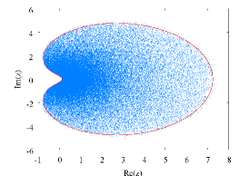
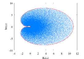
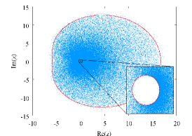
Figure 1: Scatter plot of the eigenvalues of $W_{n}$ for $\omega_{1}=\omega_{2}=\frac{1}{2}$ and $t=3$ (left), $t=4$ (middle), $t=5$ (right).

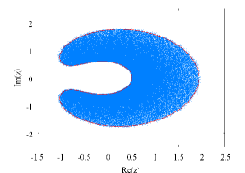
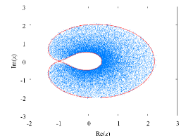
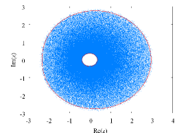
Figure 2: Same as Fig. 1 but for $\omega_{1}=\frac{1}{10}$, $\omega_{2}=\frac{1}{2}$ and $t=5$ (left), $t=\frac{20}{3}$ (middle), $t=10$ (right).

6 Conclusion

Our main objective in re-analyzing the model of [5] is our conjecture that it is a universal representative of the large-$N$ phase structure of classes of complex matrix Wilson loops. A generalization of the probability distribution allows for an interpolation between the cases where the individual factors are hermitian and unitary. We confirm, analytically and numerically, that a topological transition in the domain of non-vanishing eigenvalue density indeed occurs. Like in the unitary case, we would like to study in more detail the approach to infinite $N$ and see what the matrix model universal features of this transition are. Since a full analysis keeping the exact $N$ dependence is complicated this has not been carried to completion yet.

References

- [1] R. Narayanan, H. Neuberger, Infinite N phase transitions in continuum Wilson loop operators, JHEP 03 (2006) 064 [hep-th/0601210].
- [2] R. Narayanan, H. Neuberger, Universality of large N phase transitions in Wilson loop operators in two and three dimensions, JHEP 12 (2007) 066 [hep-th/0711.4551].
- [3] B. Durhuus, P. Olesen, The spectral density for two-dimensional continuum QCD, Nucl. Phys. B 184 (1981) 461.
- [4] R. A. Janik, W. Wieczorek, Multiplying unitary random matrices - universality and spectral properties, J. Phys. A: Math. Gen. 37 (2004) 6521 [math-ph/0312043].
- [5] E. Gudowska-Nowak, R. A. Janik, J. Jurkiewicz, M. A. Nowak, Infinite Products of Large Random Matrices and Matrix-valued Diffusion, Nucl. Phys. B 670 (2003) 479 [math-ph/0304032].