Detection of source inhomogeneity through event-by-event two-pion Bose-Einstein correlations

Abstract

We develop a method for detecting the inhomogeneity of the pion-emitting sources produced in ultra-relativistic heavy ion collisions, through event-by-event two-pion Bose-Einstein correlations. The root-mean-square of the error-inverse-weighted fluctuations between the two-pion correlation functions of single and mixed events are useful observables for the detection. By investigating the root-mean-square of the weighted fluctuations for different impact parameter regions people may hopefully determine the inhomogeneity of the particle-emitting in the coming Large Hadron Collider (LHC) heavy ion experiments.

Two-pion Hanbury-Brown-Twiss (HBT) interferometry is a useful tool for probing the space-time structure of the particle-emitting sources produced in high energy heavy ion collisions Won94 ; Wie99 ; Wei00 ; Lis05 . Because of the limitation of data statistics, the usual HBT investigations are performed for mixed events and the HBT radii are obtained by fitting the two-pion HBT correlation functions from the mixed events to Gaussian parametrized formulas.

On event-by-event basis, the density distribution of the source may be not a Gaussian distribution. An inhomogeneous particle-emitting source on event-by-event basis may be a more general case because of the fluctuating initial matter distribution in high energy heavy ion collisions Gyu97 ; Dre02 ; Ham04 ; And08 . In Ref. Zha06 , a granular source model was used to explain the Relativistic Heavy Ion Collider (RHIC) HBT results, $R_{\rm out}/R_{\rm side}\approx 1$ STA01a ; PHE02a ; PHE04a ; STA05a . The main idea of the explanation is that the evolution time for the granular sources is short and the short evolution time, which can not be averaged out after event-mixing, may lead to the HBT results $R_{\rm out}\sim R_{\rm side}$ Zha06 ; Zha04 ; Zha07 . Recent source imaging researches for the collisions of $\sqrt{s_{{}_{\rm NN}}}=200$ GeV Au+Au indicate that the pion-emitting source with the selections $40<{\rm centrality}<90\%$ and $0.20<k_{\rm T}<0.36$ GeV/c is far from a Gaussian distribution PHE07 ; Bro07 ; Yan08 . Although the long tail of the two-pion source function at large separation $r$ is believed mainly the contribution of long-lived resonances PHE07 ; Bro07 , the enhancement of the source function at small $r$ may possibly arise from the source inhomogeneity Yan08 .

For inhomogeneous particle-emitting sources, the single-event two-pion HBT correlation functions may exhibit fluctuations relative to the HBT correlation functions of mixed events Won04 ; Zha05 . Detecting and investigating this event-by-event fluctuations is important for finally determining the source inhomogeneity and understanding the initial conditions and evolution of the system in high energy heavy ion collisions.

Hydrodynamics may provide a direct link between the early state of the system and final observables and has been extensively used in high energy heavy ion collisions. In hydrodynamical calculations the system evolution is determined by the initial conditions and the equation of state (EOS) of the system. Smoothed Particle Hydrodynamics (SPH) is a suitable candidate that can be used to treat the system evolution with large fluctuating initial conditions for investigating event-by-event attributes Ham04 ; Agu01 . It has been used in high energy heavy ion collisions for a wide range of problems Ham04 ; Agu01 ; Gaz03 ; Soc04 ; Ham05 ; And06 ; And08 . In the present letter we use SPH to describe the system evolution. The system initial states are given by the NEXUS event generator Dre02 at $\tau_{0}=1$ fm/c for $\sqrt{s_{{}_{\rm NN}}}=200$ GeV Au+Au collisions at RHIC and $\tau_{0}=0.5$ fm/c for $\sqrt{s_{{}_{\rm NN}}}=5500$ GeV Pb+Pb collisions at LHC. The EOS is obtained with the entropy density suggested by QCD lattice results Bla87 ; Lae96 ; Ris96 ; Zha04 . In the EOS, the QGP phase is considered as an ideal gas of massless quarks (u, d, s) and gluons Gaz03 ; Soc04 . The hadronic gas is composed of the resonances with mass below 2.5 GeV/c², where volume correction is taken into account Gaz03 ; Soc04 . The transition temperature between the QGP and hadronic phases is taken to be $T_{\rm c}=160$ MeV, and the width of the transition is taken to be $0.1T_{\rm c}$ Ris96 .

The coordinates used in SPH are $\tau=\sqrt{t^{2}-z^{2}},\,x,\,y,$ and $\eta=(1/2)\ln[(t+z)/(t-z)]$ Ham04 ; Agu01 ; Gaz03 . They are convenient for describing the system with rapid longitudinal expansion. However, in order to investigate the whole space-time structure of the system an nonlocal coordinate frame is needed and we work in the center-of-mass frame of the system. Figure 1(a), (b), and (c) show the pictures of the transverse distributions of energy density for one $\sqrt{s_{{}_{\rm NN}}}=200$ GeV Au+Au event at $t=1$ fm/c and with impact parameter $b=0$, 5, and 10 fm, respectively. The pictures are taken for the spatial region ($|x,y|<12$ fm, $|z|<0.83$ fm) and with an exposure of $\Delta t=0.3$ fm$/c$. Fig. 1(a^′), (b^′), and (c^′) are the corresponding pictures taken at $t=5$ fm/c with the same $\Delta t$ and for the spatial region ($|x,y|<12$ fm, $|z|<1$ fm). One can see that the systems are inhomogeneous in space and time. There are many “lumps” in the systems and the number of the lumps decreases with impact parameter increasing.

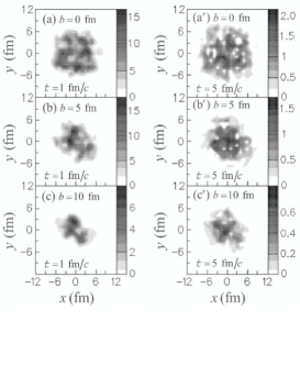
Figure 1: Transverse distributions of energy density of the systems with different impact parameters and at $t=1$ fm/c [(a)–(c)] and $t=5$ fm/c [(a^′)–(c^′)]. The unit of energy density is GeV/fm³.

Assuming that final identical pions are emitted at the space-time configuration characterized by a freeze-out temperature $T_{\rm f}$, we may generate the pion momenta according to Bose-Einstein distribution and construct the single-event and mixed-event two-pion correlation functions Zha06 ; Zha05 . Figure 2 shows the two-pion correlation functions $C(q_{\rm side},q_{\rm out},q_{\rm long})$ for the single and mixed events for $\sqrt{s_{{}_{\rm NN}}}=200$ GeV Au+Au with impact parameters $b=$ 10 fm (up panels) and $b=$5 fm (down panels). Here $q_{\rm side}$, $q_{\rm out}$, and $q_{\rm long}$ are the components of “side”, “out”, and “long” of relative momentum of pion pair Pra86 ; Ber88 . In each panel of Fig. 2, the dashed lines give the correlation functions for a sample of different single events and the solid line is for the mixed event obtained by averaging over 40 single events. In our calculations, the freeze-out temperature is taken to be 150 MeV. For each single event the total number of generated pion pairs in the relative momentum region $(q_{\rm side},q_{\rm out},q_{long}\leq 200$ MeV/c) is $N_{\pi\pi}=10^{6}$ and the numbers of the pion pairs in the relative momentum regions $(q_{i}\leq 200\,{\rm MeV/c};\,q_{j},\,q_{k}\leq 30\,{\rm MeV/c})$ are about $2.7\%N_{\pi\pi}$, where $i$, $j$, and $k$ denote “side”, “out”, and “long”.

Figure 2: Two-pion correlation functions for a sample of different single events (dashed lines) and mixed events (solid lines) with impact parameters $b=$10 fm (up panels) and $b=$5 fm (down panels).

From Fig. 2 it can be seen that the correlation functions for the single events exhibit fluctuations relative to those for the mixed events. These fluctuations are larger for bigger impact parameter. It is because that the number of the lumps in the system decreases with impact parameter and the fluctuations are larger for the source with smaller number of lumps Won04 ; Zha05 . It also can be seen that in the longitudinal direction the correlation functions exhibit oscillations which can not be smoothed out by event mixing. It is because that there are two sub-sources moving forward and backward the beam direction. This oscillations of the mixed-event correlation functions will not appear if we apply an additional cut for the initial rapidity of the “smoothed particles”, $\eta_{0}>0$ or $\eta_{0}<0$.

We have seen that the two-pion correlation functions of the single events exhibit event-by-event fluctuations. However, in the usual mixed-event HBT measurements, these fluctuations are smoothed out. In order to observe the event-by-event fluctuations, we investigate the distribution $dN/df$ of the fluctuations between the correlation functions of single and mixed events, $|C_{s}(q_{i})-C_{m}(q_{i})|$, with their error-inverses as weights Zha05 ,

$$f(q_{i})=\frac{|C_{s}(q_{i})-C_{m}(q_{i})|}{\Delta|C_{s}(q_{i})-C_{m}(q_{i})|}\,.$$ (1)

In calculations we take the width of the relative momentum $q_{i}$ bin to be 10 MeV and use the bins in the region $20\leq q_{i}\leq 200$ MeV. The up panels of Fig. 3 show the distributions of $f$ in the “side”, “out”, and “long” directions, obtained from 40 simulated $\sqrt{s_{{}_{\rm NN}}}=200$ GeV Au+Au events. The impact parameter for these events is $b=5$ fm and the number of correlated pion pairs for each of these events is $N_{\pi\pi}=10^{7}$. The solid lines are the results for the events with the fluctuating initial conditions (FIC) generated by NEXUS. Because in the last analysis the fluctuations of the single-event correlation functions are from the FIC, for comparison we also investigate the distribution $dN/df$ for the events with the smooth initial conditions (SIC) obtained by averaging over 30 random NEXUS events Ham04 ; Soc04 ; Ham05 ; And08 with the same $b$ as for the FIC. It can be seen that the $f$ distributions for FIC are much wider than the corresponding results for SIC. The down panels of Fig. 3 show the distributions of $f$ for the 40 simulated events and $N_{\pi\pi}=5\times 10^{6}$. It can bee seen that the widths of the distributions for FIC decrease with $N_{\pi\pi}$ decreasing and for $N_{\pi\pi}=5\times 10^{6}$ the distributions for FIC are still wider than those for SIC.

Figure 3: The distributions $dN/f$ for 40 events with FIC and SIC. $b=5$ fm.

Figure 4: The distributions $dN/f$ for 40 events with FIC and SIC, where $f$ are calculated for variables $q_{\rm trans}$ and $q$.

In experiments the number of correlated pion pairs in one event, $N_{\pi\pi}$, is limited. It is related to the energy $\sqrt{s_{{}_{\rm NN}}}$ of the collisions. For a finite $N_{\pi\pi}$ we have to reduce variable numbers in analysis although it will lose some details. In Fig. 4 we show the distributions of $f$ for the variables of transverse relative momentum $q_{\rm trans}$ and relative momentum $q$ of the pion pairs for the 40 simulated events with $b=5$ fm. One can see that for $N_{\pi\pi}=5\times 10^{6}$, the distributions for FIC are much wider than those for SIC both for $q_{\rm trans}$ and $q$. Even for $N_{\pi\pi}=5\times 10^{5}$, the widths for FIC are visibly larger than those for SIC. In order to examine the distributions quantitatively, we calculate the root-mean-square (RMS) of $f$. Figure 5 shows the RMS, $f_{\rm rms}$, as a function of $N_{\pi\pi}$ for the 40 simulated events for $\sqrt{s_{{}_{\rm NN}}}=200$ GeV Au+Au with $b=9$ fm (the up panels) and $b=5$ fm (the down panels), where the SIC are obtained by averaging over 100 NEXUS events. It can been seen that the values of $f_{\rm rms}$ rapidly increase with $N_{\pi\pi}$ for FIC because the errors in Eq. (1) decrease with $N_{\pi\pi}$. For FIC the results for $b=9$ fm are larger than the corresponding results for $b=5$ fm because the differences $|C_{s}(q_{i})-C_{m}(q_{i})|$ in Eq. (1) increase with $b$. For SIC the values of $f_{\rm rms}$ are almost independent from $N_{\pi\pi}$. It is because that both the differences and their errors in Eq. (1) decrease with $N_{\pi\pi}$ in the SIC case.

Figure 5: The root-mean-square of $f$ for variables $q$ and $q_{\rm trans}$ as a function of $N_{\pi\pi}$.

In Fig. 5 we only display the statistic errors which may decrease with the number of events. Moreover, in order to display the fluctuations of the single-event HBT correlation functions and the effect of FIC on the distributions of $f$, we used very large $N_{\pi\pi}$ in our calculations. At RHIC energy the event multiplicity of identical pions, $M_{\pi}$, is about several hundreds for central collisions. The order of $N_{\pi\pi}$ is about $10^{5}$ ($\sim M_{\pi}^{2}/2$). However, at the higher energy of LHC, $M_{\pi}$ will be about two thousands and the order of $N_{\pi\pi}$ will be $10^{6}$. In this case the large differences between the RMS of $f$ for inhomogeneous and homogeneous sources provide a great opportunity to detect the source inhomogeneity.

Figure 6: The root-mean-square of $f$ calculated with $q_{\rm trans}$ for 40 simulated events at LHC and RHIC energies.

Another problem in experimental data analysis is that the impact parameter $b$ is hardly to be held at a fixed value and usually be limited in a region. In such a case the large $f_{\rm rms}$ values may arise from the source inhomogeneity as well as the variation of $b$ in the region. So one should also consider the effect of the $b$ variation in inhomogeneity detections.

Figure 6(a) and (b) show the RMS of $f$ calculated with $q_{\rm trans}$ for the 40 simulated events for $\sqrt{s_{{}_{\rm NN}}}=5500$ GeV Pb+Pb with FIC and SIC, respectively. The impact parameters for the FIC events are selected randomly from the regions $b=9.0\pm 0.3$ (circle symbol) and $b=5.0\pm 0.3$ (triangle symbol), respectively. Whereas for each SIC event the SIC is constructed by averaging over 30 NEXUS events with the same impact parameter selected randomly from the $b$ region as for the FIC case. Figure 6(c) and (d) give the corresponding results for $\sqrt{s_{{}_{\rm NN}}}=200$ GeV Au+Au collisions. Our calculations indicate that the lump numbers in the sources at the LHC energy are larger than those at the RHIC energy. So the RMS values for the LHC energy are smaller than those for the RHIC energy. From Fig. 6 one can see that for FIC case (inhomogeneous sources) the RMS for the larger $b$ are higher than those for the smaller $b$. It is because that the number of lumps in the inhomogeneous source decreases with $b$ (see Fig. 1). However, for the SIC case the RMS for the two impact parameter regions are almost the same for fixed $N_{\pi\pi}$. In this case the increases of the RMS values with $N_{\pi\pi}$ are due to the fluctuations of the correlation functions arising from the variation of $b$ in their regions $\delta b$. Our calculations indicate that these increases will become flat when $\delta b\to 0$. So, one may determine the source inhomogeneity by analyzing the RMS values for different $b$ regions. For inhomogeneous sources their differences are bigger for larger $N_{\pi\pi}$. Otherwise, they are almost the same.

In summary, on event-by-event basis the initial density distribution of matter in high energy heavy ion collisions is highly fluctuating. The fluctuating initial conditions lead to event-by-event inhomogeneous particle-emitting sources. In this letter we developed a method for detecting the source inhomogeneity through event-by-event two-pion correlations. We find that the RMS of the error-inverse-weighted fluctuations $f$ are useful observables for detecting the inhomogeneity of the sources. The high identical pion multiplicity in the coming LHC heavy ion collisions provides a great opportunity to do the detections. By investigating the RMS values of $f$ for different impact parameter regions people may hopefully determine the inhomogeneity of the particle-emitting produced in the coming LHC experiments.

We thank Dr. C. Y. Wong and Dr. D. C. Zhou for helpful discussion. This research was supported by the National Natural Science Foundation of China under Contracts No. 10575024 and No. 10775024.

References

- (1) C. Y. Wong, Introduction to High-Energy Heavy-Ion Collisions (World Scientific, Singapore, 1994), Chap. 17.
- (2) U. A. Wiedemann and U. Heinz, Phys. Rept. 319, 145 (1999).
- (3) R. M. Weiner, Phys. Rept. 327, 249 (2000).
- (4) M. A. Lisa, S. Pratt, R. Soltz, U. Wiedemann, Ann. Rev. Nucl. Part. Sci. 55, 357 (2005); nucl-ex/0505014.
- (5) M. Gyulassy, D. H. Rischke, and B. Zhang, Nucl. Phys. A613, 397 (1997).
- (6) H. J. Drescher, F. M. Liu, S. Ostapchenko, T. Pierog, and K. Werner, Phys. Rev. C 65, 054902 (2002).
- (7) Y. Hama, T. Kodama, and O. Socolowski Jr, hep-ph/0407264.
- (8) R. P. G. Andrade, F. Grassi, Y. Hama, T. Kodama, and W. L. Qian, Phys. Rev. Lett. 101, 112301, 2008.
- (9) W. N. Zhang, Y. Y. Ren, and C. Y. Wong, Phys. Rev. C 74, 024908 (2006).
- (10) C. Adler et al. (STAR Collaboration), Phys. Rev. Lett. 87, 082301, 2001.
- (11) K. Adcox et al. (PHENIX Collaboration), Phys. Rev. Lett. 88, 192302, 2002.
- (12) S. S. Adler et al. (PHENIX Collaboration), Phys. Rev. Lett. 93, 152302, 2004.
- (13) J. Adams et al. (STAR Collaboration), Phys. Rev. C 71, 044906, 2005.
- (14) W. N. Zhang, M. J. Efaaf, and C. Y. Wong, Phys. Rev. C 70, 024903 (2004).
- (15) W. N. Zhang and C. Y. Wong, Int. J. Mod. Phys. E 16, 3262 (2007).
- (16) S. S. Adler et al. (PHENIX Collaboration), Phys. Rev. Lett. 98, 132301, 2007.
- (17) D. A. Brown, R. Soltz, and A. Kisiel, Phys. Rev. C 76, 044906 (2007).
- (18) Z. T. Yang, W. N. Zhang, L. Huo, and J. B. Zhang, arXiv:0808.2413.
- (19) C. Y. Wong and W. N. Zhang, Phys. Rev. C 70, 064904 (2005).
- (20) W. N. Zhang, S. X. Li, C. Y. Wong, and M. J. Efaaf, Phys. Rev. C 71, 064908 (2005).
- (21) C. E. Aguiar, T. Kodama, T. Osada, and Y. Hama, J. Phys. G 27, 75 (2001).
- (22) M. Gaździcki, M. I. Gorenstein, F. Grassi, Y. Hama, T. Kodama, and O. Socolowski Jr., Braz. J. Phys. 34, 322 (2004).
- (23) O. Socolowski Jr., F. Grassi, Y. Hama, and T. Kodama, Phys. Rev. Lett. 93, 182301 (2004).
- (24) Y. Hama, Rone P.G. Andrade, F. Grassi, O. Socolowski Jr, T. Kodama, B. Tavares, and S. S. Padula, Nucl. Phys. A774, 169 (2006).
- (25) R. Andrade, F. Grassi, and Y. Hama, Phys. Rev. Lett. 97, 202302 (2006).
- (26) J. P. Blaizot and J. Y. Ollitrault, Phys. Rev. D 36, 916 (1987).
- (27) E. Laermann, Nucl. Phys. A 610, 1 (1996).
- (28) D. H. Rischke and M. Gyulassy, Nucl. Phys A 608, 479 (1996).
- (29) S. Pratt, Phys. Rev. D 33, 72 (1986); S. Pratt, T. Csörgo, and J. Zimányi, Phys. Rev. C 42, 2646 (1990).
- (30) G. Bertsch, M. Gong, and M. Tohyama, Phys. Rev. C 37, 1896 (1988); G. Bertsch, Nucl. Phys. A 498, 173c (1989).