Testing the blazar spectral sequence: X–ray selected blazars
Abstract
We present simultaneous optical and X–ray data from Swift for a sample of radio–loud flat spectrum quasars selected from the Einstein Medium Sensitivity Survey (EMSS). We present also a complete analysis of Swift and INTEGRAL data on 4 blazars recently discussed as possibly challenging the trends of the hypothesised “blazar spectral sequence”. The SEDs of all these objects are modelled in terms of a general theoretical scheme, applicable to all blazars, leading to an estimate of the jets’ physical parameters. Our results show that, in the case of the EMSS broad line blazars, X-ray selection does not lead to find sources with synchrotron peaks in the UV/X-ray range, as was the case for X-ray selected BL Lacs. Instead, for a wide range of radio powers all the sources with broad emission lines show similar SEDs, with synchrotron components peaking below the optical/UV range. The SED models suggest that the associated IC emission should peak below the GeV range, but could be detectable in some cases by the Fermi Gamma-Ray Space Telescope. Of the remaining 4 ”anomalous” blazars, two highly luminous sources with broad lines, claimed to possibly emit synchrotron X-rays, are shown to be better described with IC models for their X-ray emission. For one source with weak emission lines (a BL Lac object) a synchrotron peak in the soft X-ray range is confirmed, while for the fourth source, exhibiting narrow emission lines typical of NLSy1s, no evidence of X-ray emission from a relativistic jet is found. We reexamine the standing and interpretation of the original “blazar spectral sequence” and suggest that the photon ambient, in which the particle acceleration and emission occur, is likely the main factor determining the shape of the blazar SED. A connection between SED shape and jet power/luminosity can however result through the link between the mass and accretion rate of the central black hole and the radiative efficiency of the resulting accretion flow, thus involving at least two parameters.
keywords:
galaxies: active - galaxies: jets - radiation mechanisms: non–thermal1 Introduction
The Spectral Energy Distributions (SED) of blazars from radio to gamma–rays exhibit remarkable properties, in particular a “universal” structure consisting of two broad humps. A systematic compilation of multiwavelength data for three complete samples, two selected in the radio band (2Jy FSRQ and 1 Jy BL Lacs) and one in X–rays (Einstein Slew Survey BL Lacs) was performed by Fossati et al. (1998). Note that, at the time, the results from the Compton Gamma-Ray Observatory (CGRO) were still under study, while very few objects had been detected in the TeV band, thus the data at high energies were rather incomplete.
The derived SEDs were averaged in fixed radio luminosity bins, irrespective of sample membership or classification (BL Lac vs. FSRQ). The result was the well known “Spectral Sequence” (a series of 5 average SEDs, “sequence” in the following) showing the peaks of the two spectral components shifting systematically to higher frequencies with decreasing luminosity. For brevity we will refer to SEDs with synchrotron peak below or above the optical range as ”red” or ”blue” SEDs respectively.
It has to be stressed that the derived average SEDs, by themselves, only represent the spectral properties of the considered samples and do not contain further implications; however the fact that, despite the mixing of different samples and classifications, the average SEDs show systematic trends, possibly driven by the radio power suggests an underlying regularity of behaviour of jets in very different objects. Understanding this behavior could lead to a more profound comprehension of the jets’ radiation mechanisms and physics.
Ghisellini et al. (1998) modelled a large number of individual sources with sufficient data at high energies with a simple general scheme: a single emission region, moving with bulk Lorentz factor , contains relativistic electrons emitting via synchrotron radiation the lower energy spectral component; the same electrons up scatter synchrotron photons as well as photons from an external radiation field producing the high energy spectral component. The electron spectrum is computed assuming a broken power law injection spectrum and taking into account radiative energy losses.
With these minimal assumptions the “sequence” of spectral properties translates into a parameter sequence, in which the energy of the electrons radiating at the SED peaks is higher for lower values of the (comoving) total magnetic field plus photon energy densities, due to the reduced energy losses. This interpretation of the “sequence” concept and following developments (Ghisellini, Celotti & Costamante 2002; Costamante & Ghisellini 2002) led to successful predictions of the best candidates for TeV detection (see Wagner 2008 for a recent review).
On the other hand, the phenomenological “sequence” is likely affected by observational biases (Maraschi and Tavecchio 2001 (ASP CS Vol 227)). Significant efforts were made to construct new samples of blazars with different thresholds and selection criteria (e.g., Laurent-Muehleisen et al. 1999, Caccianiga & Marchã 2004, Massaro et al. 2005, Landt et al. 2006, Giommi et al. 2007a, Turriziani et al. 2007, Healey et al. 2008, Massaro et al. 2008) and some discrepant objects were found (see Padovani 2007 for a review on the challenges to the blazar sequence). In particular Caccianiga & Marchã (2004) evidenced the existence of sources with relatively low radio power, but X-ray to radio ratios similar to those of FSRQs.
In a somewhat different line of approach the group lead by Valtaoja developped a technique to estimate the beaming parameters (Doppler factors Lorentz factors and viewing angles) of blazar jets from the radio properties alone (Valtaoja et al. 1999, Lahteenmaki, Valtaoja & Wiik 1999, Lahteenmaki & Valtaoja 1999). Basing on extensive monitoring data at high radio frequencies (22 and 37 GHz) these authors compute ”apparent” brightness temperatures using light travel times inferred from variability as sizes for the emission region. Comparing the results with the theoretical maximum brightness temperature allowed by the SSC process they derive the Doppler factor of the emission region and further use the apparent superluminal speeds to determine the bulk Lorentz factor and the viewing angle. This procedure is correct, however one has to keep in mind that the results obtained refer to the radio emitting regions of the jet, which do not coincide with the regions emitting the high energy radiation (e.g. Ghisellini et al. 1998; Sikora 2001). Moreover in the analysis of the SEDs of a large number of BL Lac objects Nieppola et al. (2006) fit the data in the full (radio to gamma-ray) frequency range available with a single parabolic curve, thus their determination of the ”peak frequency” of the SED cannot be compared with our approach. In Nieppola et al. (2008) however, the parabolic fits are not forced to include the X-ray and higher energy data, yielding peak frequencies that can be compared with ours. We will discuss their results in the Discussion Section.
One of the problems in the “sequence” assembly was the lack of an X–ray selected sample of flat–spectrum radio quasars. Wolter & Celotti (2001) selected and discussed a sample of FSRQ within the X-ray selected sample of radio Loud AGN from the Einstein Medium Sensitivity Survey (EMSS). They found that the average broad–band spectral indices of these X–ray selected FSRQs were consistent with those of the radio selected FSRQs within the “sequence”. However, a study of their SEDs was not possible due to insufficient spectral data.
Here, we present Swift observations of the 10 X–ray brightest objects in the Wolter & Celotti sample as well as a full analysis of Swift data for 4 blazars recently claimed to be at odds with the sequence scheme. We model the SEDs of the 14 objects following Ghisellini, Celotti & Costamante (2002), deriving estimates of important physical quantities for their jets. Finally, in the light of these new results, we discuss the present standing and interpretation of the blazar “spectral sequence”. Preliminary results were given in Maraschi et al. (2008). The scheme of the paper is as follows: Sect. 2 gives information on the selected sources and Sect. 3 describes the data and analysis methods. Sect. 4 details the general spectral modelling procedure. The results are presented in Sect. 5. A general discussion is given in Sect. 6 while Sect. 7 offers the conclusions
2 The sources
2.1 The X-ray selected Radio Loud AGN sample from the Einstein Medium Sensitivity Survey
Wolter & Celotti (2001) selected 39 Radio–Loud, broad line AGN from the X–ray EMSS sample (Gioia et al. 1990, Stocke et al. 1991). Of these, 20 had a measured radio spectral index and their broad band properties were compared to those of classical radio selected flat spectrum quasars. Their broad band indices (, ) were found to be similar to those of FSRQ. This is at odds with the case of BL Lac objects, which occupy very different regions in the , plane depending on whether they derive from X–ray or radio selection. On the other hand, broad–band indices give only a global information, which may be ambiguous (see below). We therefore decided to exploit the unique capabilities of the Swift satellite to observe the ten X–ray brightest FSRQs of the EMSS sample in order to derive their X–ray spectrum together with simultaneous optical data allowing a reliable snapshot of the optical to X-ray SED. Observations were performed within the filler program. The data gathered and analysis methods are described in Sect. 3.
2.2 Controversial Sources
In addition to the EMSS sources, we include in our analysis and discussion four sources of controversial classifications put forward by other authors: two ultraluminous, high–redshift, broad line quasars recently discovered, SDSS J (, Giommi et al. 2007b) and MG3 J(, Bassani et al. 2007) have been claimed, on the basis of their broad-band spectral indices, to show a synchrotron peak in hard X–rays. If confirmed, these claims would imply strong violations of the sequence scheme.
Two other cases concern blazars of intermediate luminosities, namely RX J (, Giommi 2008) and RGB J (, Padovani et al. 2002), which show synchrotron peaks in the X–ray band and, in addition, exhibit emission lines, weak in the first source and pronounced, but narrow, in the second one. For these 4 objects, all the existing data obtained with Swift and, in the case of MG3 J also the data obtained with INTEGRAL were systematically reanalysed to produce a data set as homogeneous and complete as possible.
3 Data analysis
All the data presented here were analyzed in the same way to guarantee a homogeneous treatment. The common procedures adopted for the analysis are described below.
3.1 Swift
The data from all three instruments onboard Swift, namely BAT, XRT and UVOT (Gehrels et al. 2004), have been processed and analyzed with HEASoft v. 6.3.2 with the CALDB release of November 11, 2007. The observation log is reported in Tables 1.
The X–ray Telescope XRT ( keV, Burrows et al. 2005) data were analyzed using the xrtpipeline task, selecting single to quadruple pixel events (grades ) in the photon-counting mode. Individual spectra from multiple pointings, together with the proper response matrices, were integrated by using the addspec task of FTOOLS. The final count spectra were then rebinned in order to have at least counts per energy bin, depending on the available statistics, and spectral fits were performed with simple power law models and galactic . In only three cases additional absorption or a broken power law fit was required. The average spectral parameters are reported in Table 2.
The sensitivity of the hard X–ray detector BAT (optimized for the keV energy band, Barthelmy et al. 2005) is generally insufficient to detect extragalactic sources in short exposures, unless for bright states. Therefore, in order to get meaningful signal-to-noise ratios we combined all the available pointings for a given source. All the shadowgrams from pointings of the same source were binned, cleaned from hot pixels and background (flat-field), and deconvolved. The intensity images were then integrated by using the variance as weighting factor. No detection with sufficient signal-to-noise ratio has been found for any source with the available exposures and upper limits at (corrected for systematic errors) in two energy bands ( and keV) have been calculated (see Table 3).
Data from the optical/ultraviolet telescope UVOT (Roming et al. 2005) were analyzed using the uvotmaghist task with source regions of for optical filters and for the UV filters, while the background was extracted from a source-free annular region with inner radius equal to (optical) or (UV) and outer radius from to , depending on the presence of nearby contaminating sources. In the cases of MS , SDSS J, RX J, and MG3 J the presence of a nearby source prevents the use of a background region with annular shape; therefore, a circular source free region with radius was selected. We added a error in flux (corresponding to about magnitudes) to take into account systematic effects. The summary of average magnitudes per filters is reported in Table 4.
3.2 INTEGRAL
The hard X–ray ( keV) data on MG3 J were obtained from the IBIS/ISGRI detector onboard INTEGRAL (Lebrun et al. 2003). They were analyzed with the Off-line Scientific Analysis (OSA) v. 7.0, whose algorithms for IBIS are described in Goldwurm et al. (2003), using the latest calibration files (v. 7.0.2).
The source was observed serendipitously during the revolutions (May , ) and (July , ) for a total exposure of ks. The results are reported in Table 3. The joint data from the INTEGRAL/ISGRI together with those of Swift/XRT, covering an energy range of keV, can be still fit with a single power-law model with and additional absorption of cm-2, to mime the low-energy photon deficit. The fit gives a for degrees of freedom. The results are consistent with the values for Swift/XRT only, reported in Table 2.
3.3 Two-point spectral indices
Two point spectral indices , , between fixed radio/optical/X-ray frequencies have been computed for all sources, to facilitate comparison with other samples.
The two-point optical/X–ray spectral index has been calculated according to the formula (Ledden & O’Dell 1985):
| (1) |
where and can be the radio ( GHz), optical (at Hz corresponding to Å, filter) and X–ray (at Hz corresponding to keV) flux densities, respectively. The flux densities have been K–corrected by multiplying for the factor , where is the spectral index of . An average spectral index has been used for radio and optical frequencies, with values of and (Pian & Treves 1993). The and X-ray flux density have been measured from the spectral fitting of Swift/XRT data reported in Table 2.
The radio flux densities at GHz have been extracted from NED111http://nedwww.ipac.caltech.edu/ or from radio catalogs available through HEASARC222http://heasarc.gsfc.nasa.gov/. When the GHz flux density was not available (a very few cases), we have extrapolated the requested value from the GHz flux density.
The Swift/UVOT flux densities have been calculated from the observed magnitudes, dereddened with the from NED and extrapolated to other frequencies by means of the extinction law by Cardelli et al. (1989), and converted by using the zeropoints given in the HEASoft package.
The derived values are reported in Table 4.
4 SED Models
The observed SEDs of all sources were modelled following the theoretical scheme developed by Ghisellini, Celotti & Costamante (2002) and also used by Celotti and Ghisellini (2008, CG08), where a more detailed description can be found.
Briefly, the observed radiation is postulated to originate in a single dissipation zone of the jet, described as a cylinder of cross sectional radius and thickness (as seen in the comoving frame) . We assume a conical jet with aperture angle , the dissipation is assumed to always occur at .
The relativistic particles are assumed to be injected throughout the emitting volume for a finite time with total injected power in relativistic particles in the comoving frame of the emission region. The observed SED is obtained from the particle distribution resulting from the cumulative effects of the injection and radiative energy loss processes at the end of the injection, at , when the emitted luminosity is maximised.
The finite injection duration, together with the magnetic and radiation energy densities seen by the particles, determine the energy above which the injected particle spectrum is affected by the radiative cooling processes.
The particle injection function is assumed to extend from to , with a broken power–law shape with slopes and below and above .
If (fast cooling regime) the resulting particle spectrum is given by
| (2) |
In the opposite case (slow cooling regime), radiative losses affect the spectral shape only at higher energies , yielding:
| (3) |
The relativistic electrons radiate via the synchrotron and the Inverse Compton mechanisms. The latter includes the SSC and the external Compton (EC) processes. The external radiation for the EC process is assumed to derive from the accretion disk emission scattered and reprocessed in the surrounding broad line region (Sikora et al. 1994).
With the distributions given above, the synchrotron and IC peaks in the SED are due to electrons with Lorentz factor, , determined by the injected distribution and the radiative losses: in the fast cooling regime as long as . When , (provided that ). In the slow cooling regime, instead, (if ).
In most of the sources considered here the data indicate the presence of a prominent optical/UV excess that one can identify with the disk emission and then can be used to estimate . The disk emission is assumed to be a black body, peaking at frequency Hz. Besides this black body UV component, we also consider the emission of the X–ray corona. This X–ray component is assumed to have , to start a factor 30 below the UV bump, and to have an exponential cutoff at 150 keV. When no optical/UV excess is apparent we still include a possible accretion disk (that can be considered as an upper limit). The external radiation field is derived assuming for the Broad Line Region a luminosity and a size derived from the relation
| (4) |
where erg s-1, in approximate agreement with Kaspi et al. (2007). Since , the radiation energy density of the BLR photons, as measured by an observer inside the BLR at rest with respect to the black hole, is constant, and equal to erg cm-3. In the comoving frame, however, the radiation energy density will be enhanced by a factor. When is smaller then the dissipation zone , we completely neglect any external radiation.
The essential parameters of the model and their role can summarized as follows:
-
•
, , and determine the injected relativistic particle distribution;
-
•
the magnetic field and the radiation energy density determine , the energy of the cooling break, and thus the particle spectrum after cooling. includes the contribution of both the synchrotron photons and the external photons. In the comoving frame , therefore also the bulk Lorentz factor is involved.
-
•
the viewing angle , together with , determines the Doppler (beaming) factor , and then the boosting of the entire SED;
-
•
the ratio determines the EC to synchrotron luminosity ratio.
The SED peak frequencies (, ) depend mainly on the shape of the particle spectrum. If is high (low cooling) and is above the optical band and the SSC dominates the high energy emission. If is low (strong cooling) 10–100 and then is very much below the optical band, often below the self–absorption frequency, and the EC mechanism produces the high energy component.
Finally, the power carried by the jet in different forms (radiation, magnetic field, relativistic electrons, cold protons) can be computed from the model parameters as:
| (5) |
where , , ,
We refer to CG08 for a recent estimate and discussion of the jet powers for a large number of blazars.
5 Results
5.1 The EMSS sample
In all cases the X-ray spectra are well fit by simple power laws with photon indices ranging from 1.8 to 1.3 and the index, which indicates the relative intensity of the X-ray to optical emission, varies from 0.9 to 1.6. None of the objects is detected in the hard X–rays with BAT.
In radio–quiet AGN, where the optical as well as X–ray emission derive from an accretion disk, this ratio is on average (see, e.g., Vignali et al. 2003). Thus, the lower values of for the EMSS sample, i.e. the high ratios of X–ray to optical fluxes (see Table 4) point to a significant contribution from the jet in the X–ray band. This conclusion is reinforced by the derived spectral indices in the X–ray band () which are unusually hard for normal, even radio loud but not flat spectrum, quasars (, see Grandi et al. 2006, Guainazzi et al. 2006). Therefore, the observed X-ray emission can be attributed to the combined contributions from the accretion disk corona plus a harder X-ray component deriving from Inverse Compton scattering of external photons (EC) off relativistic electrons in the jet. We recall that all the objects in the sample have Broad Line Regions providing seeds for the EC process.
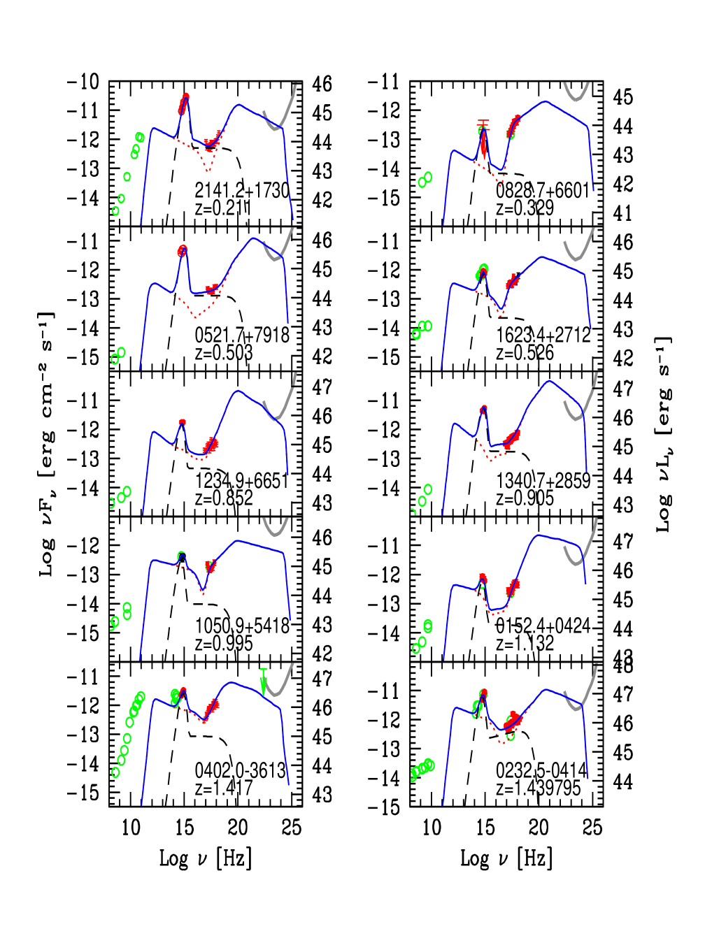
The optical and X–ray fluxes derived from Swift for the X–ray selected radio-loud AGN are shown in Fig. 1 (in order of redshift), together with historical radio and optical data, and theoretical models for the full SEDs. The high optical/UV fluxes and hard X-ray spectra indicate that the UV to X-ray SED have a concave shape as commonly observed for FSRQs. Therefore, in all cases the synchrotron peak frequency should fall below the UV range (red SED). On the other hand, the lack of data in the IR-submm region does not allow to set stronger observational constraints on its location.
It is noteworthy that the two objects with the highest , MS and MS , have relatively low radio luminosity ( erg s-1). This suggests that the jets in these sources could be either intrinsically weak or seen at intermediate angles, therefore not strongly beamed (see also Landt et al. 2008). Indeed, the unified model predicts that blazars at intermediate angle should exist (in large numbers). Sources with subluminous jets were not present in the samples used to construct the sequence, likely because the high threshold in radio flux selected only the most beamed sources.
The X–ray selected AGN considered here, whose radio emission was in some sense measured “a posteriori”, have radio fluxes on average around mJy and radio luminosities in the range erg s-1, about one order of magnitude lower than the range covered by the FSRQs in the sequence. The optical fluxes, indicative of the accretion disk emission, correspond instead to luminosities of erg s-1, well in to the typical quasar range. An even lower radio power interval was explored by Caccianiga and Marcha (2004), though without spectral information.
MS is extreme in the opposite way, in that the optical luminosity is lower than the X–ray one and the X–ray spectrum is extremely hard (). The Galactic absorption column is cm-2 and the X–ray spectrum does not show any hint of additional absorption, suggesting that the source is intrinsically faint at optical wavelengths.
The SED models shown in Fig. 1 (continuous/blue lines) were computed as described in Section 3. As noted above the main observational constraints are that the synchrotron peak should fall below the UV range and that the jet contribution in X-rays should have a hard slope. Observational data below the optical and above the X-ray range are lacking so that the models cannot be more strongly constrained. According to our SED models the peak of the high energy emission, always dominated by the EC process, falls around 1-10 MeV, unusually low compared to known –ray blazars. –ray observations would be extremely important to confirm these models: the sensitivity curve of the Fermi GRT,for a 1 yr exposure, shown for comparison on each SED, indicates that several of these sources may be detected in the near future.
The model parameters adopted are reported in Table 5.
Since the lack of high energy (hard X–ray and –ray) data leaves some freedom in the choice of the fitting parameters we present also examples of alternative models for the SEDs.
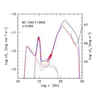
In Fig. 2 two models for the SED of MS , both fitting the optical and X–ray data equally well, are compared. The first (same as in Fig. 1) predicts a –ray flux well above the FermiGRT sensitivity; the second predicts a lower –ray flux, just below the FermiGRT sensitivity limit. The parameters for the two models are quite similar (see Tab. 5).
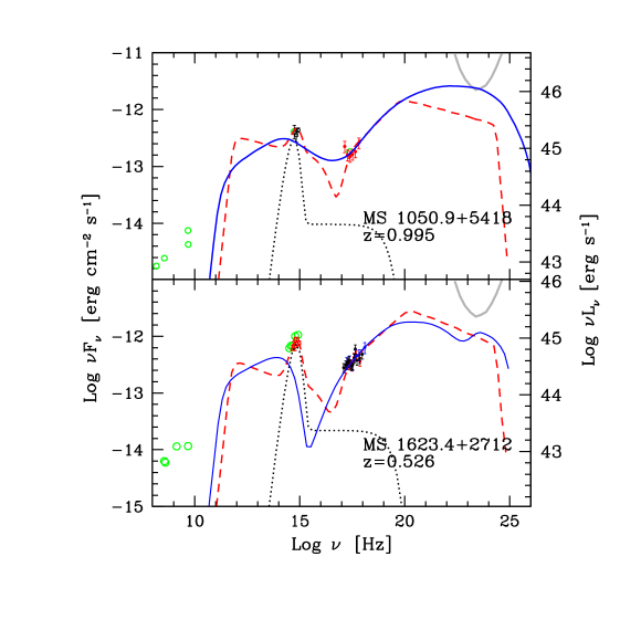
In Fig. 3 alternative SED models (solid lines) for MS and MS are shown. Both sources are characterized by a relatively small accretion disk luminosity, hence a small , a “normal” X–ray to optical luminosity ratio and a “normal” X–ray slope (as opposed to e.g. MS 0828.7+6601, which has a relatively stronger, and harder, X–ray component). We hypothesize here that the dissipation region of the jet is beyond the BLR (i.e. ), contrary to what assumed for the models shown in Fig. 1. Then, in the absence of external photons, the cooling threshold is high and the synchrotron emission peaks close to (but not above) the optical band, while the whole high energy emission from X-rays to -rays is produced by the SSC (instead of EC) process. Note that the injection spectrum is also different from the previous models, in that changes from 1 to 400 and 300 for the two sources respectively (see Tab. 5). As a consequence the jet powers computed for the latter models are significantly reduced (Tab. 6).
These examples illustrate the ambiguities in our models when and are “normal”, and the accretion disk luminosity is relatively modest, suggesting a small broad line region. It is clear from Fig. 3 that additional data, especially between the sub–mm and the optical region of the SED are needed to discriminate between these alternatives. In the following we discuss the results assuming in all the cases the parameters obtained with the standard external Compton model.
5.2 Controversial blazars
5.2.1 Two high red-shift “red” blazars
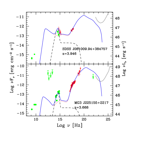
Two high redshift powerful blazars recently discovered (SDSS J, Giommi et al. 2007b; MG3 J, Bassani et al. 2007, Falco et al. 1998), both showing conspicuous broad lines, have been claimed to possibly exhibit a synchrotron peak in the X–ray band at variance with the sequence scheme. Our reanalysis of all the existing Swift and INTEGRAL data is summarized in the Tables and the results are shown in Fig. 4. For SDSS J the Swift observations yield only upper limits in the optical UV range. Therefore the optical fluxes measured by the SDSS, though not simultaneous to the X-ray data, are also shown in Fig. 4. In both cases the hard X-ray spectra suggest a concavity of the optical to X–ray SEDs, pointing to an inverse-Compton origin of the X–ray/hard X–ray emission. Though both objects have , less than the conventional threshold value of 0.78 taken to distinguish HBL from LBL, the ”red” nature of their SEDs seems clear even with these limited data.
The case of MG3 J discovered with INTEGRAL is extraordinary: the X–ray to hard X–ray component dominates the optical emission by more than one order of magnitude. Attributing the latter component to synchrotron emission would require implausibly high values of both magnetic field and particle energies. The SED of this source is very similar to that of Swift J () discovered by the BAT instrument on board Swift (Sambruna et al. 2006a).
Clearly, a hard X–ray selection favors the discovery of objects with an extremely dominant hard X–ray component. It is nevertheless interesting that blazars with such extreme dominance of the high energy emission component actually exist.
Our model SEDs are shown in (Fig. 4) For SDSS J, although the wavelength coverage is poor, the hard X-ray spectrum measured by Swift strongly disfavors both a synchrotron or SSC interpretation of the X-ray emission. We therefore propose a model with synchrotron peak at low energies and a strong EC component. On the other hand the peak energy of the EC component is uncertain as in the case discussed above for MS1340.7.
For MG3 J the INTEGRAL data define well the lower energy side of the EC component: this branch of the SED reveals the low energy end of the electron distribution. The SED model is sufficiently determined by the data and the peak energy of the EC component is unlikely to be higher.
5.2.2 Two luminous “blue” blazars
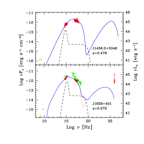
The SEDs for RX J and RGB J including all the data analysed here, are shown in Fig. 5. Here the data confirm the “blue” nature of the SEDs as discussed already in Padovani et al. (2002) and Giommi (2008) respectively. In both cases the synchrotron peak falls in the UV to X-ray range as typical for ”High energy peaked” BL Lacs (HBL).
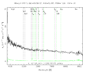
Indeed RX J can be classified as a BL Lac, since its optical spectrum from the SDSS (see Fig. 6) shows a blue continuum and very weak emission lines, with equivalent width Å333According to the line measurements available in the SDSS server at http://cas.sdss.org/astrodr6/en. We note also that the radio source previously associated with this object is probably a misidentification: a bright, compact flat-spectrum radio source in the field, about 44 arcsec to the east of the SDSS BL Lac object, dominates the radio flux in this region. In the best image from the FIRST, at 1.4 GHz, the field source is 168 mJy, whereas the BL Lac object is only 9.5 mJy (T. Cheung, private communication). The latter value for the radio flux is shown in Fig. 5. RX J is highly luminous, but still comparable to the well known HBL PKS in the bright state recently observed (Foschini et al. 2007, 2008).
The SED model for this object shown in Fig. 5 formally assumes , however there is no indication that a broad line region exists at all in this object. Also the possible contribution of an accretion disk is only an upper limit. The cooling threshold is very high, as well as the break energy of the injection spectrum which coincides with .
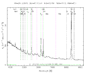
The case of RGB J is intriguing. Its optical spectrum, also from the SDSS, is shown in Fig. 7. The emission lines are pronounced, but “narrow” ( km/s, Komossa et al. 2006), typical of Narrow-line Seyfert 1 galaxies. Estimates of the mass of the central BH are in the range M⊙ (Komossa et al. 2006). This is unusual for a radio loud source and in particular for blazars. However mass estimates for NLSy1s may have to be revised (Marconi et al. 2008, Decarli et al. 2008). In fact the whole case of NLSy1 and particularly that of radio loud NLSy1 is the subject of active debate (e.g. Malizia et al. 2008, W. Yuan et al. 2008). Specifically RGB J is only moderately radio loud and its X-ray emission spectrum showing a broken power law spectrum with spectral indices and below and above 0.5 keV does not point unambiguously to a jet contribution. The X-ray emission could be driven by its NLSy1 nature (Komossa et al. 2006)
Nevertheless we modelled the SED of this source assuming a jet contribution and negligible radiative losses in the dissipation region (). The radiation energy density is thus due to magnetic field and synchrotron photons only. The resulting SSC component has low luminosity.
6 Discussion
6.1 Model parameters and correlations
It is interesting to compare the (model independent) two point spectral index with quantities derived from the modelling for the EMSS sample. describes the ratio of the optical to X-ray emission. For the “red” SEDs of this sample the optical is often dominated by the accretion disk emission while the X-ray contribution in excess of the accretion disk corona can derive from the jet, therefore is a measure of their relative strength.
We find from the modelling that correlates with the viewing angle (Fig. 8) as well as (inversely) with the Doppler factor (not shown). We recall that and enter the models in different ways so that both are determined in the fits: is then derived from the first two. The two correlations are not independent as the value of is almost constant ranging between 10 and 15.
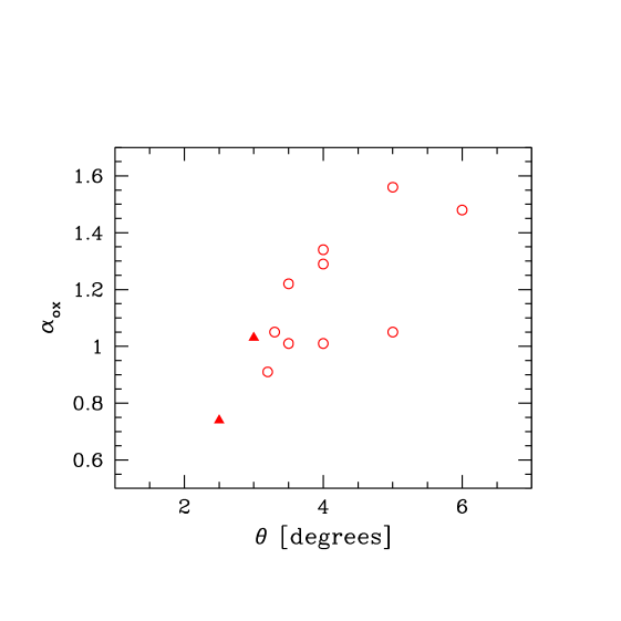
The - correlation agrees with the initial expectation that relatively weak jet contributions could derive from intermediate viewing angles. However also correlates inversely with the estimated jet intrinsic power, so that the two effects, a lower degree of beaming or a lower intrinsic jet power, cannot be disentangled and probably coexist. On the other hand, does not correlate with , indicating that it is the relative jet ”strength”, either due to the viewing angle or to the intrinsic power, that may drive these correlations.
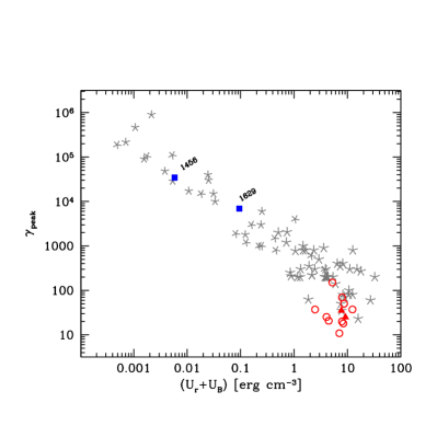
The most important parameter determining the shape of the SED is , the energy of electrons radiating the peak synchrotron luminosity. The relation between and the radiation energy density as seen in the emission region frame, , is shown in Fig. 9, for the objects discussed here. Values derived for the blazars modelled in CG08 are also shown for comparison. The new objects fall well within the parameter sequence defined by the previous sample. Therefore, despite the different selection criteria, X-ray selection as opposed to radio selection for FSRQ and selections aimed at finding sources breaking the sequence trends, the spectral sequence holds in terms of physical parameters.
The “red” objects tend to cluster at one end, with rather low . The clustering can result from the assumption (adapted from Kaspi et al. 2007) of an almost constant intrinsic radiation energy density in the BLR: since the magnetic field value is limited by the high Compton to synchrotron ratio, (which varies by a factor 2 for between 10 and 15) cannot be exceeded substantially.
Blue SEDs are obtained for small , such that is high, while the opposite is true for red SEDs. This is a result of the feed-back introduced by including radiative cooling in modelling the energy distribution of the relativistic electrons. However this is not the only important difference between the electron distributions producing blue and red SEDs. Another major difference is at the lower electron energies: in fact, below , the assumed electron distribution is extremely hard () so that the total number of electrons is small and their average energy much higher than in the case of red SEDs (see Table 6).
6.2 Jet powers
The total jet power, , computed from the models (see Sect.4) is shown vs. the luminosity of the accretion disk (estimated from the data) in Fig. 10, together with values previously derived for other blazars (Maraschi & Tavecchio 2003, Sambruna et al. 2006b). The two quantities tend to correlate for the red SEDs. Moreover the value of is of the order of 10 times the disk luminosity, corresponding to an approximate equality of the jet power and the accretion power (for an assumed radiative efficiency of the accretion process of 10% appropriate for an optically thick flow). This represents on one hand an interesting consistency check on the models. In fact the bulk Lorentz factor, size, magnetic field, particle densities and spectra in the dissipation region are chosen to satisfy the SED constraints, including clearly the observed fluxes/luminosities, but the jet power is a global quantity that is computed a posteriori. Moreover the new data and models increase significantly the number of sources in which a comparison of the jet power with the accretion power is possible and confirms the substantial balance between the two.
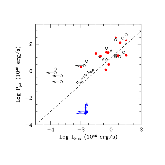
The value of the power for jets with red SEDs depends quite strongly on the minimum energy of the injected electrons, , which is often poorly constrained. For red SEDs the X-ray emission derives from the EC process of relatively low energy electrons thus a lower limit can be obtained. Moreover in several cases, could be inferred from detailed fits of X-ray spectra showing a break in the X-ray range. Such breaks have sometimes been interpreted as absorption by cold gas (e.g. Cappi et al. 1997, Fiore et al. 1998, Fabian et al. 2001a,b, Bassett et al. 2004) but could represent instead the low energy ”end” of the electron distribution (e.g. Tavecchio et al. 2007). With the latter interpretation is found to be in the range 1-10, thus supporting the high power values (Tavecchio et al. 2000, Maraschi & Tavecchio 2003, CG08). These powers rest on the assumption of 1 cold proton per electron, but are independently required by the fact that the power directly radiated by the jet is larger than the power in relativistic leptons and magnetic field (CG08).
For jets with blue SEDs the jet power derived from the present models is substantially lower, due to the smaller number and higher mean energy of particles in the assumed relativistic electron population. The uncertainty on the amount of low energy electrons in the jet is however quite large because radiation from this branch of the electron distribution is not observable: its synchrotron emission is covered by the larger fluxes due to the outer regions of the jet and its SSC emission falls in the hard X-ray - soft gamma-ray region of the spectrum which is difficult to observe. Note that from Table 6 the total kinetic power from the ”blue” jets is hardly sufficient to account for the emitted radiation, thus the assumed spectra lead to a lower limit in the estimate of the jet powers.
As a result, in the – plane, the ”blue” objects modelled here fall well below the = 10 line. In the same diagram the grey open circles with upper limits to the disk luminosities (horizontal arrows) represent BL Lacs from Maraschi & Tavecchio (2003) for which an electron distribution with slope 2 extending down to a Lorentz factor of 1 was assumed below the peak energy.
Despite the large uncertainties about the powers of the ”blue” objects, it is interesting that the ”red” blazars discussed here which result from independent selection criteria in the X-ray/hard X-ray band confirm the results previously obtained for radioselected FSRQ.
Very different results were obtained by Nieppola et al. (2008) for a large sample of Blazars using beaming corrections derived from brightness temperatures at high radio frequencies using variability to estimate the sizes of the emission regions. This technique gives information on the Doppler factors for the radioemitting regions in AGN. They find an anticorrelation between Doppler factor and peak frequency of the synchrotron component such that the objects with higher peak frequency are less beamed. As a result the ”intrinsic” powers of objects with large peak frequency (i.e. ”blue” objects) are higher than those of ”red” objects.
While models of TeV emitting blazars require Doppler factors as large as 10-50 (e.g. Krawczynski et al. 2002, Konopelko et al. 2003, Finke et al. 2008, Aharonian et al. 2008, Tagliaferri et al. 2008), VLBI observations show very small, subluminal motions (e.g. Piner, Pant & Edwards 2008). These two evidences can be reconciled assuming that the jet strongly decelerates from the blazar region to the VLBI scale, from which most of the radio emission originates (Georganopoulos et al. 2003, Ghisellini et al. 2005). This would also fit in with the scenario in which FR I jets decelerate on moderate scale lengths while FR II jets may remain relativistic up to very large scales (e.g. Tavecchio 2007). Therefore the Doppler factors obtained by Nieppola et al. (2008) for the jet radio emitting regions are probably much smaller than the Doppler factors in the optical-to--ray emitting region especially in the case of high peaked BL Lac objects.
7 Conclusions
We have analysed and modelled new data for the SEDs of blazars including the first X-ray selected sample of Radio-loud Quasars and a few more blazars claimed to possibly challenge the “blazar spectral sequence”. The first, model independent, conclusion is that the conventional separation of different “types” of blazars according to their two point spectral indices () can be deceiving, due to the complexity and variety of the SEDs: for instance the traditional criterion to distinguish between blue and red SEDs fails in the case of SDSS J and MG3 J which have , yet this is not due to synchrotron emission in the X-ray band but to an extremely dominant Compton component. Results from the Fermi Gamma-ray Telescope will be critical in confirming our interpretation
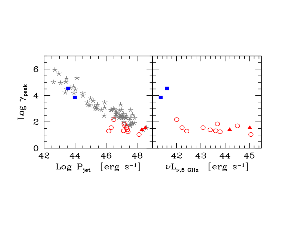
The “blazar spectral sequence” concept still holds in terms of a parameter sequence. In Fig.11 (left panel) the parameter computed from SED models is plotted vs. total jet power also computed from the models. A “sequence” (i.e. correlation) is still apparent between these two quantities, We stress that is related to the spectral shape while is a global quantity related to the emitted luminosity.
However (Fig.11, right panel) does not show a clear correlation with the observed radio luminosity, which was the basic quantity used in building the spectral sequence. This is likely due to the fact that at lower flux thresholds intrinsically luminous but less beamed objects enter the samples causing a mix of lower luminosity due to lower intrinsic power or lower beaming. This ambiguity could probably be solved with high resolution radio observations.
The spectral sequence requires that different “types” of blazars, from FSRQ to low–energy peaked BL Lac Objects (LBLs) to HBLs, have SED peaks at increasing frequencies. This is accounted for by increasing values of , derived in our models with the assumption that radiative cooling affects the electron distribution becoming less important as the radiation energy density around the dissipation region decreases. However the particle distributions needed to account for red and blue SEDs respectively differ not only at the high energy end but also at the low energy end. Blue SEDs require an electron population with higher ”average” energy, perhaps pointing to different injection/acceleration mechanisms.
The present results show that even X-ray selection does not lead to find ”blue” quasars as was the case for X-ray selected BL Lac samples (see also Landt et al. 2008). This strengthens the conclusion that when a bright accretion disk is present the SED is always ”red”. However, if the initial samples suggested luminosity/power as a fundamental parameter in determining the SEDs’ systematics, the present study suggests that the fundamental condition that separates “red” SEDs from “blue” ones is the intensity of the radiation field in the emission region, which is dominated by reprocessed photons from an accretion disk, if present. The relation with luminosity/power could be indirect, due to the fact that a bright accretion disk forms only for high values of the accretion rate in Eddington units (e.g. ), while the absence of it (RIAF, Radiatively Inefficient Accretion Flows) occurs for , thus at lower power for a fixed mass of the accreting Black Hole. Thus, the original picture of blazar SEDs, as a one parameter family governed by luminosity, should be revised including the mass of the accreting Black Hole as an additional important parameter. A new scheme along these lines has been recently suggested by Ghisellini & Tavecchio (2008).
Acknowledgements
We thank an anonymous referee for useful comments. This research has made use of data obtained from the High Energy Astrophysics Science Archive Research Center (HEASARC), provided by NASA’s Goddard Space Flight Center.
This research has made use of the NASA/IPAC Extragalactic Database (NED) which is operated by the Jet Propulsion Laboratory, California Institute of Technology, under contract with the National Aeronautics and Space Administration.
Funding for the SDSS and SDSS-II has been provided by the Alfred P. Sloan Foundation, the Participating Institutions, the National Science Foundation, the U.S. Department of Energy, the National Aeronautics and Space Administration, the Japanese Monbukagakusho, the Max Planck Society, and the Higher Education Funding Council for England. The SDSS Web Site is http://www.sdss.org/. The SDSS is managed by the Astrophysical Research Consortium for the Participating Institutions. The Participating Institutions are the American Museum of Natural History, Astrophysical Institute Potsdam, University of Basel, University of Cambridge, Case Western Reserve University, University of Chicago, Drexel University, Fermilab, the Institute for Advanced Study, the Japan Participation Group, Johns Hopkins University, the Joint Institute for Nuclear Astrophysics, the Kavli Institute for Particle Astrophysics and Cosmology, the Korean Scientist Group, the Chinese Academy of Sciences (LAMOST), Los Alamos National Laboratory, the Max-Planck-Institute for Astronomy (MPIA), the Max-Planck-Institute for Astrophysics (MPA), New Mexico State University, Ohio State University, University of Pittsburgh, University of Portsmouth, Princeton University, the United States Naval Observatory, and the University of Washington.
We acknowledge funding from ASI/INAF with contract I/088/06/0.
References
- [2008] Aharonian F., et al., 2008, A&A, 481, L103
- [2005] Barthelmy S.D., Barbier L.M., Cummings J.R., et al., 2005, Space Sci. Rev. 120, 143
- [2005] Bassani L., Landi R., Malizia A., et al., 2007, ApJ 669, L1
- [] Bassett L. C., Brandt W. N., Schneider D. P., Vignali C., Chartas G., & Garmire G. P. 2004, AJ, 128, 523
- [2005] Burrows D.N., Hill J.E., Nousek J.A., et al., 2005, Space Sci. Rev. 120, 165
- [2004] Caccianiga A. & Marchã M.J.M., 2004, MNRAS 348, 937
- [] Cappi M., Matsuoka M., Comastri A., Brinkmann W., Elvis M., Palumbo G. G. C., & Vignali C. 1997, ApJ, 478, 492
- [1989] Cardelli J.A., Clayton G.C., Mathis J.S., 1989, ApJ 345, 245
- [2008] Celotti A. & Ghisellini G., 2008, MNRAS 385, 283
- [2002] Costamante L. & Ghisellini G., 2002, A&A, 384, 56
- [1995] Dondi L. & Ghisellini G., 1995, MNRAS 273, 583
- [] Fabian A. C., Celotti A., Iwasawa K., McMahon R. G., Carilli C. L., Brandt, W. N., Ghisellini G., & Hook I. M. 2001a, MNRAS, 323, 373
- [Fabian et al.(2001)] Fabian A. C., Celotti A., Iwasawa K., & Ghisellini G. 2001b, MNRAS, 324, 628
- [1998] Falco E. E., Kochanek C. S., Munoz J. A., 1998, ApJ, 494, 47
- [2008] Decarli R., Dotti M., Fontana M., Haardt F., 2008, MNRAS, 386, L15
- [2008] Finke J., Dermer C., Böttcher M., 2008, ApJ, accepted [arXiv: 0802.1529]
- [] Fiore F., Elvis M., Giommi P., & Padovani P. 1998, ApJ, 492, 79
- [2007] Foschini L., Ghisellini G., Tavecchio F., et al., 2007, ApJ 657, L81
- [2008] Foschini L., Treves A., Tavecchio F., et al., 2008, A&A, 484, 35
- [1998] Fossati G., Maraschi L., Celotti A., Comastri A., Ghisellini G., 1998, MNRAS 299, 433
- [2004] Gehrels N., Chincarini G., Giommi P., et al., 2004, ApJ 611, 1005
- [2003] Georganopoulos M., Kazanas D., 2003, ApJ, 594, L27
- [1998] Ghisellini G., Celotti A., Fossati G., Maraschi L., Comastri A., 1998, MNRAS 301, 451
- [2002] Ghisellini G., Celotti A., Costamante L., 2002, A&A 386, 833
- [2005] Ghisellini G., Tavecchio F., Chiaberge M., 2005, A&A, 432, 401
- [2008] Ghisellini G. & Tavecchio F., 2008, MNRAS, 387, 1669
- [1990] Gioia I. M., Maccacaro T., Schild R. E., Wolter A., Stocke J. T., Morris S. L., Henry J. P., 1990, ApJS, 72, 567
- [2007a] Giommi P., Capalbi M., Cavazzuti E., et al., 2007a, A&A 468, 571
- [2007b] Giommi P., Massaro E., Padovani P., et al., 2007b, A&A 468, 97
- [2008] Giommi P., 2008, Mem. SAIt 79, 154
- [2003] Goldwurm A., David P., Foschini L., et al., 2003, A&A 411, L223
- [2006] Grandi P., Malaguti G. & Fiocchi M., 2006, ApJ 642, 113
- [2006] Guainazzi M., Siemiginowska A., Stanghellini C., et al., 2006, A&A 446, 87
- [2008] Healey S.E., Romani R.W., Cotter G., et al., 2008, ApJS 175, 97
- [2005] Kalberla P.M.W., Burton W.B., Hartmann D. A., et al., 2005, A&A, 440, 775
- [2007] Kaspi S., Brandt W.N., Maoz D., Netxer H., Schneider D.P. & Shemmer O., 2007, ApJ, 659, 997
- [2007] Katarzyński K. & Ghisellini G., 2007, A&A 463, 529
- [2006] Komossa S., Voges W., Xu D., et al., 2006, ApJ 132, 531
- [2003] Konopelko A., Mastichiadis A., Kirk J., de Jager O. C., Stecker F. W., 2003, ApJ, 597, 851
- [2002] Krawczynski H., Coppi P. S., Aharonian F., 2002, MNRAS, 336, 721
- [2005] Kusunose M. & Takahara F., 2005, ApJ 621, 285
- [1999] Lähteenmäki A., Valtaoja E., 1999, ApJ, 521, 493
- [1999] Lähteenmäki A., Valtaoja E., Wiik K., 1999, ApJ, 511, 112
- [2008] Landt H., Padovani P., Giommi P., Perri M., Cheung C. C., 2008, ApJ, 676, 87
- [2006] Landt H., Perlman E., Padovani P., 2006, ApJ 637, 183
- [1999] Laurent-Muehleisen S.A., Kollgaard R.I., Feigelson E.D., et al., 1999, ApJ 525, 127
- [2003] Lebrun F., Leray J.-P., Lavocat P., et al. 2003, A&A 411, L141
- [1985] Ledden J.E. & O’Dell S.L., 1985, ApJ 298, 630
- [2008] Malizia A. et al. 2008, MNRAS, in press (arXiv:0806.4824)
- [2003] Maraschi L. & Tavecchio F., 2003, ApJ 593, 667
- [2008] Maraschi L., Ghisellini G., Tavecchio F., Foschini L., Sambruna R.M., 2008, Proceedings of the Conference “High-Energy Processes in Relativistic Outflows” (Dublin, 2007). [arXiv:0802.1789]
- [] Marconi A., Axon D. J., Maiolino R., Nagao T., Pastorini G., Pietrini P., Robinson A., Torricelli G., 2008, ApJ, 678, 693
- [2005] Massaro E., Sclavi S., Giommi P., Perri M., Piranomonte S., 2005, Multifrequency Catalogue of Blazars, vol. 1: 0h-6h, Roma, Aracne Editrice
- [2008] Massaro E., Giommi P., Leto C., et al., 2008, Multifrequency Catalogue of Blazars, vol. 2: 6h-12h, Roma, Aracne Editrice
- [2006] Nieppola E., Tornikoski M., Valtaoja E., 2006, A&A, 445, 441
- [2008] Nieppola E., Valtaoja E., Tornikoski M., Hovatta T., Kotiranta M., 2008, A&A, submitted (arXiv:0803.0654)
- [2002] Padovani P., Costamante L., Ghisellini G., Giommi P. & Perlman E., 2002, ApJ 581, 895
- [2007] Padovani P., 2007, Ap&SS 309, 63
- [1993] Pian E. & Treves A., 1993, ApJ 416, 130
- [2008] Piner B. G., Pant N., Edwards P. G., 2008, ApJ, 678, 64
- [2005] Roming P.W.A., Kennedy T.E., Mason K.O., et al., 2005, Space Sci. Rev. 120, 95
- [2006] Sambruna R.M., Markwardt C.B., Mushotzky R.F., et al., 2006a, ApJ 646, 23
- [\citeauthoryearSambruna et al.2006] Sambruna R. M., Gliozzi M., Tavecchio F., Maraschi L., Foschini L., 2006b, ApJ, 652, 146
- [1994] Sikora M., Begelman M. C., Rees M. J., 1994, ApJ, 421, 153
- [2001] Sikora M., 2001, ASPC, 227, 95
- [2002] Sikora M., Błażejowski M., Moderski R., Madejski G., 2002, ApJ 577, 78
- [1991] Stocke J. T., Morris S. L., Gioia I. M., Maccacaro T., Schild R., Wolter A., Fleming T. A., Henry J. P., 1991, ApJS, 76, 813
- [2008] Tagliaferri G., et al., 2008, ApJ, 679, 1029
- [2007] Tavecchio F., 2007, Ap&SS, 311, 247
- [] Tavecchio F., Maraschi L., Ghisellini G., Kataoka J., Foschini L., Sambruna R. M., Tagliaferri G., 2007, ApJ, 665, 980
- [] Tavecchio F., et al. 2000, ApJ, 543, 535
- [1998] Tavecchio F., Maraschi L., Ghisellini G., 1998, ApJ 509, 608
- [1974] Toor A. & Seward F.D., 1974, AJ 79, 995
- [2007] Turriziani S., Cavazzuti E., Giommi P., 2007, A&A 472, 699
- [1999] Valtaoja E., Lähteenmäki A., Teräsranta H., Lainela M., 1999, ApJS, 120, 95
- [2003] Vignali C., Brandt W.N. & Schneider D.P., 2003, AJ 125, 433
- [2008] Wagner R. M., 2008, MNRAS, 385, 119
- [2001] Wolter A. & Celotti A., 2001, A&A 371, 527
- [2008] Yuan W. et al. 2008, ApJ, in press (arXiv:0806.3755)
| Source | ObsID | Date |
|---|---|---|
| MS | ||
| MS | ||
| MS | ||
| MS | ||
| MS | ||
| MS | ||
| MS | ||
| MS | ||
| MS | ||
| MS | ||
| SDSS J | ||
| MG3 J | ||
| RX J | ||
| RGB J | ||
| Source | Exposure | /dof | |||||||
|---|---|---|---|---|---|---|---|---|---|
| MS | |||||||||
| MS | |||||||||
| MS | |||||||||
| MS | |||||||||
| MS | |||||||||
| MS | |||||||||
| MS | |||||||||
| MS | |||||||||
| MS | |||||||||
| MS | |||||||||
| SDSS J | |||||||||
| MG3 J | |||||||||
| RX J | |||||||||
| RGB J |
| Source | Exposure | ||
|---|---|---|---|
| MS | |||
| MS | |||
| MS | |||
| MS | |||
| MS | |||
| MS | |||
| MS | |||
| MS | |||
| MS | |||
| MS | |||
| SDSS J | |||
| MG3 J | |||
| MG3 J | |||
| RX J | |||
| RGB J |
-
∗
INTEGRAL observation.
| Source | V | B | U | UVW1 | UVM2 | UVW2 | |||
| MS | 0.61 | 0.75 | |||||||
| MS | 0.43 | 0.70 | |||||||
| MS | 0.60 | 0.74 | |||||||
| MS | 0.38 | 0.73 | |||||||
| MS | 0.81 | ||||||||
| MS | 0.57 | 0.71 | |||||||
| MS | 0.48 | 0.71 | |||||||
| MS | 0.39 | 0.69 | |||||||
| MS | 0.60 | 0.75 | |||||||
| MS | 0.49 | 0.83 | |||||||
| SDSS J | 0.56 | ||||||||
| MG3 J | 0.52 | 0.59 | |||||||
| RX J | 0.42 | 0.55 | |||||||
| RGB J | 0.35 | 0.66 |
| Source | Note | |||||||||||||
| (1) | (2) | (3) | (4) | (5) | (6) | (7) | (8) | (9) | (10) | (11) | (12) | (13) | (14) | (15) |
| MS 0152.4+0424 | 1.132 | 10 | 1.5e-2 | 14 | 3.3 | 2.4 | 1 | 3e3 | 18 | 3.2 | 5 | 220 | 11 | |
| MS 0232.5-0414 | 1.439 | 18 | 3.0e-2 | 13 | 4.0 | 7 | 1 | 6e3 | 50 | 3.3 | 100 | 1.e3 | 6 | |
| MS 0402.0-3613 | 1.417 | 12 | 2.3e-2 | 11 | 4.0 | 8 | 4 | 1e4 | 11 | 3.4 | 40 | 700 | 11 | |
| MS 0521.7+7918 | 0.503 | 10 | 1.0e-2 | 13 | 6.0 | 2 | 150 | 8e3 | 150 | 3.5 | 7 | 300 | 18 | |
| MS 0828.7+6601 | 0.329 | 2 | 6.0e-5 | 14 | 3.2 | 3 | 1 | 1e4 | 37 | 3.45 | 0.1 | 25 | 37 | |
| MS 1050.9+5418 | 0.995 | 10 | 1.5e-3 | 12 | 3.5 | 5 | 1 | 1e4 | 21 | 3.2 | 2 | 180 | 21 | |
| 18 | 2.5e-3 | 12 | 3.5 | 0.12 | 400 | 2e5 | 7e3 | 3.5 | 2 | 140 | 7e3 | |||
| MS 1234.9+6651 | 0.852 | 9 | 7.0e-3 | 12 | 3.5 | 3 | 15 | 5e3 | 25 | 3.6 | 6.5 | 320 | 25 | |
| MS 1340.7+2859 | 0.905 | 14 | 2.5e-2 | 13 | 4.0 | 3 | 70 | 3e3 | 70 | 3.6 | 29 | 500 | 8 | below GLAST |
| 14 | 2.0e-2 | 14 | 4.5 | 5 | 40 | 3e3 | 40 | 3.7 | 25 | 550 | 9 | above GLAST | ||
| MS 1623.4+2712 | 0.526 | 10 | 1.6e-3 | 11 | 5.0 | 3 | 1 | 1e4 | 37 | 3.3 | 1 | 150 | 37 | |
| 15 | 3.6e-4 | 11 | 3.5 | 0.1 | 300 | 1e4 | 2.1e4 | 3.6 | 1 | 100 | 2e4 | |||
| MS 2141.2+1739 | 0.211 | 10 | 9.0e-4 | 12 | 5.0 | 6.5 | 20 | 1.5e4 | 20 | 2.4 | 4.5 | 200 | 12 | |
| SDSSJ081009.94+384757.0 | 3.946 | 16 | 0.1 | 14 | 3.0 | 5 | 25 | 1.5e3 | 25 | 3.8 | 100 | 1000 | 6 | |
| MG3 J225155+2217 | 3.668 | 20 | 0.2 | 15 | 2.5 | 0.7 | 35 | 1e3 | 35 | 3.8 | 21 | 500 | 6 | |
| RX J1456.0+5048 | 0.478 | 15 | 2.0e-4 | 15 | 3.0 | 0.3 | 3.5e4 | 5e5 | 3.5e4 | 3.4 | 0.2 | 45 | 1e4 | |
| RGB J1629+401 | 0.272 | 10 | 1.1e-4 | 10 | 4.0 | 1.5 | 7e3 | 1e5 | 7e3 | 3.5 | 0.25 | 50 | 930 |
| Source | Note | ||||||
| (1) | (2) | (3) | (4) | (5) | (6) | (7) | (8) |
| MS | 3.15 | 0.04 | 0.42 | 1.11 | 253 | 8.1 | |
| MS | 4.92 | 0.73 | 10.03 | 0.68 | 152 | 8.2 | |
| MS | 2.29 | 0.33 | 4.16 | 2.90 | 1301 | 4.1 | |
| MS | 1.73 | 0.04 | 0.25 | 0.29 | 31 | 17.6 | |
| MS | 1.20e-2 | 1.53e-4 | 2.64e-2 | 3.24e-2 | 21 | 2.9 | |
| MS | 0.20 | 2.67e-2 | 1.25 | 0.24 | 129 | 3.4 | |
| 0.39 | 2.90e-2 | 2.51e-3 | 1.27 | 14.4 | 162 | ||
| MS | 1.02 | 2.71e-2 | 0.39 | 1.10 | 236 | 8.6 | |
| MS | 4.32 | 9.73e-2 | 1.11 | 0.78 | 142 | 10 | below GLAST |
| 3.80 | 0.195 | 3.59 | 1.22 | 254 | 8.8 | above GLAST | |
| MS | 0.19 | 1.50e-2 | 0.41 | 3.66 | 203 | 3.3 | |
| 5.60e-2 | 6.0e-3 | 1.0e-3 | 0.96 | 15 | 117 | ||
| MS | 0.12 | 1.38e-2 | 2.27 | 5.52e-2 | 12.4 | 8.2 | |
| SDSS J | 19.79 | 0.44 | 4.69 | 7.10 | 1996 | 6.5 | |
| MG3 J | 50.05 | 2.12e-2 | 0.16 | 12.77 | 3320 | 7 | |
| RX J | 3.26e-2 | 2.13e-2 | 1.70e-2 | 1.17e-2 | 7.1e-3 | 3049 | |
| RGB J | 1.13e-2 | 1.03e-2 | 8.39e-2 | 2.23e-3 | 9.3e-3 | 442 |