Magnetic phase boundaries Exchange and superexchange interactions Rare earth metals and alloys

Magnetic Order Beyond RKKY in the Classical Kondo Lattice

Abstract

We study the Kondo lattice model of band electrons coupled to classical spins, in three dimensions, using a combination of variational calculation and Monte Carlo. We use the weak coupling ‘RKKY’ window and the strong coupling regime as benchmarks, but focus on the physically relevant intermediate coupling regime. Even for modest electron-spin coupling the phase boundaries move away from the RKKY results, the non interacting Fermi surface no longer dictates magnetic order, and weak coupling ‘spiral’ phases give way to collinear order. We use these results to revisit the classic problem of $4f$ magnetism and demonstrate how both electronic structure and coupling effects beyond RKKY control the magnetism in these materials.

The Kondo lattice model describes local moments on a lattice coupled to an electron band. Such local moments arise from electron correlation and Hunds coupling in the $d$ shells of transition metals or the $f$ shells of rare earths. Although historically the ‘Kondo lattice’ arose as the lattice version [1] of the Kondo impurity problem, and refers to $S=1/2$ moments coupled to conduction electrons, there are also systems with local electron-spin coupling where the moment is due to a spin with $2S\gg 1$. In that case the quantum fluctuations of the local moment, and the Kondo effect itself, are not relevant. Such a system can be described by a classical Kondo lattice model (CKLM). This limit is relevant for a wide variety of materials, e.g, the manganites [2], where $S=3/2$ moments couple to itinerant electrons via Hunds coupling, or $4f$ metals [3, 4, 5, 6], e.g, Gd with $S=7/2$, or the Mn based dilute magnetic semiconductors [7] where $S=5/2$. In some of these materials, notably the manganites and the magnetic semiconductors, the coupling scale is known to be large, while in the $f$ metals they have been traditionally treated as being weak.

The CKLM involves the ordering of ‘classical’ spins, but the effective interaction between spins is mediated by electron delocalisation and cannot be described by a short range model. In fact the major theoretical difficulty in analysing these systems is the absence of any simple classical spin model. Nevertheless, there are two limits where the CKLM is well understood. (a). When the electron-spin coupling is small, one can perturbatively ‘integrate out’ the electrons and obtain the celebrated Ruderman-Kittel-Kasuya-Yosida (RKKY) model [8]. The effective spin-spin interaction in this limit is oscillatory and long range, controlled by the free electron susceptibility, $\chi_{0}({\bf q})$, and the magnetic ground state is generally a spiral. (b). When the electron-spin coupling is very large compared to the kinetic energy, the ‘double exchange’ (DE) limit, the electron spin is ‘slaved’ to the orientation of the core spin and the electronic energy is minimised by a ferromagnetic (FM) background [9]. This leads intuitively to a spin polarised ground state.

In many materials the ratio of coupling to hopping scale is $\geq 1$, but not quite in the double exchange limit. In that case one has to solve the coupled spin-fermion model from first principles. Doing so, particularly in three dimensions and at finite temperature, has been a challenge. We study this problem using a combination of variational calculation and full spin-fermion Monte Carlo.

Our principal results are the following: (i) We are able to map out the magnetic ground state all the way from the RKKY limit to double exchange, revealing the intricate evolution with coupling strength. (ii) We demonstrate that the phase boundaries depend sensitively on electronic hopping parameters. This is not surprising in the RKKY regime, but the dependence at stronger coupling is unknown. (iii) We use our results to revisit the classic $4f$ magnets, widely modelled as RKKY systems, and suggest that with increasing $4f$ moment, the effective coupling in these systems pushes them beyond the RKKY regime. We work out the signatures of this ‘physics beyond RKKY’.

Model: The Kondo lattice model is given by

$$H=-\sum_{{\langle ij\rangle}\sigma}t_{ij}c^{\dagger}_{i\sigma}c_{j\sigma}-\mu\sum_{i}n_{i}-J\sum_{i}{\vec{\sigma}}_{i}.{\bf S}_{i}$$ (1)

We will use $t=1$ as the nearest neighbour hopping amplitude, and explore a range of $t^{\prime}$, the next neighbour hopping, on a cubic lattice. Changing $t^{\prime}$ will allow us to explore changes in the (bare) Fermi surface, and particle-hole asymmetry. $\mu$ is the chemical potential, and $J>0$ is the local electron-spin coupling. We assume the ${\bf S}_{i}$ to be classical unit vectors, and absorb the magnitude of the core spin into $J$ wherever necessary. ${\vec{\sigma}}_{i}$ is the electron spin operator. We work with $\mu$, rather than electron density $(n)$, as the control variable so that regimes of phase separation (PS) can be detected, and study the magnetic properties for varying $n$, $t^{\prime}/t$, $J/t$, and temperature $T/t$.

Although there have been many studies in the ‘double exchange’ ($J/t\rightarrow\infty$) limit [10], the attempts to explore the full $n-J-T$ phase diagram have been limited. $(a)$ An effective action obtained from the CKLM via gradient expansion [11] has been analysed. This mapped out some of the commensurate and spiral phases in two dimensions, where the phases are fewer. It did not explore the finite temperature physics, e.g, the $T_{c}$ scales, and seems to be inaccurate when handling commensurability effects near $n=1$. $(b)$ The model has been studied within dynamical mean field theory [12] (DMFT), and the broad regimes of ferromagnetism, antiferromagnetism (AFM), and incommensurate order have been mapped out. Unfortunately the effective ‘single site’ character of DMFT does not allow a characterisation of the incommensurate phases and misses out on the richness of the phase diagram. The loss of information about spatial fluctuations also means that critical properties, either in magnetism or transport, cannot be correctly captured. $(c)$ An ‘equation of motion’ approach [13] has been employed to study general finite S spins coupled to fermions, and results have been obtained in the classical limit as well. However, except the ferro and antiferromagnetic phases other magnetic states do not seem to have been explored. $(d)$ The full spin-fermion Monte Carlo, using exact diagnolisation, has been employed [14] in one and two dimensions but severe size limitations prevent access to non trivial ordered states.

Method: The problem is technically difficult because it involves coupled quantum and classical degrees of freedom, and there is in general no equivalent classical spin Hamiltonian. The probability distribution for spin configurations is given by $P\{{\bf S}\}\propto Tr_{c,c^{\dagger}}e^{-\beta H}$ so the ‘effective Hamiltonian’ is $H_{eff}\{{\bf S}\}=-{1\over{\beta}}log~{}Tr_{c,c^{\dagger}}e^{-\beta H}$, the fermion free energy in an arbitrary background $\{{\bf S}_{i}\}$. It cannot be analytically calculated except when $J/t\ll 1$.

When $J/t\ll 1$, the (free) energy calculated perturbatively to ${\cal O}(J^{2})$ leads to the RKKY spin Hamiltonian [8], $H^{eff}_{RKKY}=\sum_{ij}J_{ij}{\bf S}_{i}.{\bf S}_{j}$, where $J_{ij}\sim J^{2}\chi^{0}_{ij}$ and $\chi^{0}_{ij}$ is the non local susceptibility of the free $(J=0)$ electron system. $\chi^{0}_{ij}$ is long range and oscillatory. We will analyse this model to understand the weak coupling phases. At strong coupling, $J/t\rightarrow\infty$, there is no exact analytic $H_{eff}$ but we can construct approximate self consistent models [15] of the form $H^{eff}_{DE}=-\sum_{\langle ij\rangle}D_{ij}\sqrt{1+{\bf S}_{i}.{\bf S}_{j}}$, with the $D_{ij}$ related to the electronic kinetic energy. Unfortunately, when $J\sim{\cal O}(t)$ neither the RKKY model nor the DE approximation are valid. This regime requires new tools and we will use a combination of (i) variational calculation (VC) [16] for the magnetic ground state, and (ii) spin-fermion Monte Carlo using a ‘travelling cluster’ approximation [17] (TCA-MC) at finite temperature.

For the variational calculation we choose a simple parametrisation [18] for the spin configuration: $S_{iz}=\alpha$, $S_{ix}=\sqrt{1-\alpha^{2}}~{}cos{{\bf q}.{\bf r}_{i}}$ and $S_{iy}=\sqrt{1-\alpha^{2}}~{}sin{{\bf q}.{\bf r}_{i}}$. This encompasses the standard ferromagnet and antiferromagnet, as well as planar spiral phases, canted ferromagnets, and A and C type antiferromagnets. For a fixed $\mu$ and $J$ we compute the electronic energy ${\cal E}(\alpha,{\bf q},\mu)$ and minimise it with respect to $\alpha$ and ${\bf q}$. The electronic density at the chosen $\mu$ is computed on the minimised state. Since the magnetic background only mixes electronic states $|{\bf k},\uparrow\rangle$ and $|{\bf k}-{\bf q},\downarrow\rangle$ the electronic eigenvalues $\epsilon^{\pm}({\bf k},{\bf q})$ are simple, and only an elementary numerical sum is required to calculate ${\cal E}(\alpha,{\bf q},\mu)=\sum_{{\bf k},\pm}\epsilon^{\pm}({\bf k},{\bf q})\theta(\mu-\epsilon^{\pm}({\bf k},{\bf q}))$.

While the VC provides a feeling for the possible ground states, it has the limitation that (i) it samples only one family of (periodic) functions in arriving at the ground state, and (ii) finite temperature properties, e.g, the magnetisation and the critical temperature are not accessible. For this we ‘anneal’ the system towards the equilibrium distribution $P\{{\bf S}\}\propto Tr_{c,c^{\dagger}}e^{-\beta H}$ using the TCA based Monte Carlo. In this method the acceptance of a spin update is determined by diagonalising a cluster Hamiltonian constructed around the update site, and avoids iterative diagonalisation [14] of the full system. We can access system size $\sim 10^{3}$ using a moving cluster of size $4^{3}$.

The TCA captures phases with commensurate wavevector ${\bf Q}$ quite accurately, but access to the weak coupling incommensurate phases is poor. To get an impression of the ordering temperature for these phases we compute the energy difference $\Delta{\cal E}(n,J)={1\over N}({\cal E}_{disord}-{\cal E}_{ord})$, between the ordered state and a fully spin disordered state in a large system. ${\cal E}_{ord}$ is calculated from the variational ground state, and ${\cal E}_{disord}$ by diagonalising the electron system in a fully spin disordered background on a large lattice. $\Delta{\cal E}(n,J)$ is the ‘condensation energy’ of the ordered state, and provides a crude measure of the effective exchange and $T_{c}$. Where we could compare the trend to MC data, the agreement was reasonable.

Results: The results of the variational calculation in the ‘symmetric’ ($t^{\prime}=0$) case are shown in Fig.1. We employed a grid with upto $40^{3}$ ${\bf k}$ points, and have checked stability with respect to grid size. Let us analyse the weak and strong coupling regimes first before getting to the more complex intermediate coupling regime.

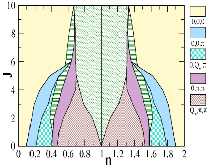
Figure 1: Colour online: Magnetic ground state for the particle-hole symmetric model $(t^{\prime}=0)$ for varying electron density $(n)$ and electron-spin coupling $(J)$. The phases are characterised by their ordering wavevector ${\bf Q}$, indicated by the colour code in the legend to the right, and their net magnetisation $\alpha$ (if any). Among the ‘commensurate’ phases, ${\bf Q}=\{0,0,0\}$ is the usual ferromagnet, $\{0,\pi,\pi\}$ and $\{\pi,\pi,\pi\}$ are antiferromagnets with no net magnetisation, while the $\{0,0,\pi\}$ antiferromagnet has $\alpha=0$ for $J\rightarrow 0$ but picks up finite magnetisation with increasing $J$. At $n=1$ the system is always a ${\bf Q}=\{\pi,\pi,\pi\}$ antiferromagnet. The incommensurate phases have ordering wavevectors $\{Q_{x},Q_{y},Q_{z}\}$ of which at least one component is neither $0$ nor $\pi$. For such phases the exact wavevector depends on the value of $n$ and $J$. For example, for $J\rightarrow 0$ the (blue) checkerboard region in the left hand corner, to the right of ${\bf Q}=\{0,0,\pi\}$, has wavevector ${\bf Q}=\{0,Q_{y},\pi\}$, where $Q_{y}$ varies from $0$ to $\pi$ as one moves left to right. The (green) shaded regions in the phase diagram, not indicated in the legend, are windows of phase separation. No homogeneous phases are allowed in these regions. The results in this figure are based on a variational calculation using a $20^{3}$ ${\bf k}$ point grid, and cross-checked with data on $40^{3}$.

(i) RKKY limit: The key features for $J/t\rightarrow 0$ are: (i) the occurence of ‘commensurate’ planar spiral phases, with wavenumber ${\bf Q}$ which is $\{0,0,0\}$, or $\{0,0,\pi\}$, etc, over finite density windows, (ii) the presence of planar spirals with incommensurate ${\bf Q}$ over certain density intervals, (iii) the absence of any phase separation, i.e, only second order phase boundaries, and (iv) the presence of a ‘G type’, ${\bf Q}=\{\pi,\pi,\pi\}$, antiferromagnet at $n=1$. Although the magnetic state is obtained from the variational calculation, much insight can be gained by analysing the $H^{eff}_{RKKY}$. Since the spin-spin interaction is long range it is useful to study the Fourier transformed version $H^{eff}_{RKKY}\equiv\sum_{\bf q}{\tilde{J}}_{\bf q}|{\bf S}_{\bf q}|^{2}$, where ${\tilde{J}}_{\bf q}=\sum_{i-j}J_{ij}e^{i{\bf q}.{\bf R}_{ij}}$ and ${\bf S}_{\bf q}=\sum_{i}{\bf S}_{i}e^{i{\bf q}.{\bf R}_{i}}$. The coupling ${\tilde{J}}_{\bf q}=J^{2}\chi_{0}({\bf q},n)$ is controlled by the spin susceptibility, $\chi_{0}({\bf q},n)$, of the $J=0$ tight binding electron system. For our choice of variational state the minimum of $H^{eff}$ corresponds to the wavevector at which $\chi_{0}({\bf q},n)$ has a maximum. We independently computed $\chi_{0}({\bf q},n)$ and confirmed [19] that the wavevector ${\bf Q}(n)$ obtained from the VC closely matches the wavevector ${\bf q}_{max}(n)$ of the peak in $\chi_{0}({\bf q},n)$. The absolute maximum in $\chi_{0}({\bf q},n)$ remains at ${\bf q}=\{0,0,0\}$, as the electron density is increased from $n=0$, and at a critical density ${\bf q}_{max}$ shifts to $\{0,0,\pi\}$. With further increase in density ${\bf q}_{max}$ evolves through $\{0,q,\pi\}$ to the C type $\{0,\pi,\pi\}$, then $\{q,\pi,\pi\}$, and finally the G type AFM with $\{\pi,\pi,\pi\}$, where the Fermi surface is nested. The absence of ‘conical’ phases, with finite $(\alpha)$ and a spiral wavevector, is consistent with what is known in the RKKY problem.

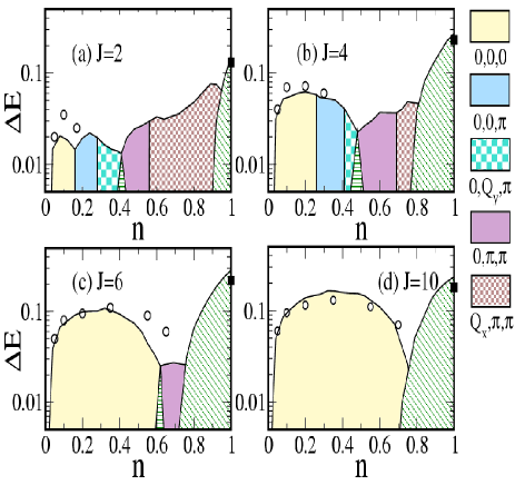
Figure 2: Colour online: The finite temperature phase diagram in the particle-hole symmetric case, for various $J$. Panels (a)-(d) show the different ordered phases and their estimated transition temperature as we move from the weak coupling to the double exchange limit. The legend for the phases is shown on the right. The transition temperatures are based either on Monte Carlo results (shown as symbols), or the $\Delta{\cal E}$ estimate (firm lines) described in the text. Notice that the $T_{c}$ for the ferromagnetic, ${\bf Q}=\{0,0,0\}$, phase increases (and saturates) with increasing $J$. At $n=1$ the order is at ${\bf Q}=\{\pi,\pi,\pi\}$ and the corresponding $T_{c}$ initially increases with increasing $J$ and then decreases. Except for ${\bf Q}=\{0,0,0\}$ and $\{\pi,\pi,\pi\}$ other phases vanish by the time $J/t=10$. The Monte Carlo estimate of ferromagnetic $T_{c}$ are shown as circles, while that of the antiferromagnet is marked on the $n=1$ axis by a square symbol. As in Fig.1 the (green) shaded regions indicate phase separation.

There is no phase separation, i.e, discontinuities in $n(\mu)$, for $J/t\rightarrow 0$ since the $\mu-n$ relation is that of the underlying tight binding system and free of any singularity. The phase transitions with changing $n$ are all second order. With growing $J/t$, however, some phase boundaries become first order and regimes of PS will emerge.

(ii) Strong coupling: For $J/t\rightarrow\infty$, it makes sense to quantise the fermion spin at site ${\bf R}_{i}$ in the direction of the core spin ${\bf S}_{i}$, and project out the ‘high energy’ unfavourable state. This leads to an effective spinless fermion problem whose bandwidth is controlled by the average spin overlap $\langle{\bf S}_{i}.{\bf S}_{j}\rangle$ between neighbouring sites. The overlap is largest for a fully polarised state, and the FM turns out to be the ground state at all $n\neq 1$. At $n=1$ ‘real hopping’ is forbidden so the fermions prefer a G type AFM background to gain kinetic energy ${\cal O}(t^{2}/J)$ via virtual hops.

The FM and G type AFM have a first order transition between them with a window of phase separation, easily estimated at large $J/t$. The fully polarised FM phase has a density of states (DOS) which is simply two 3D tight binding DOS with splitting $J$ between the band centers. If we denote this DOS as $N_{FM}(\omega,J)$ then the energy of the FM phase is ${\cal E}_{FM}(\mu,J)=\int_{-\infty}^{\mu}N_{FM}(\omega,J)\omega d\omega$, and the particle density is $n(\mu,J)=\int_{-\infty}^{\mu}N_{FM}(\omega,J)d\omega$. There will be corresponding expressions when we consider electrons in the $\{\pi,\pi,\pi\}$ AFM background, with DOS $N_{AFM}(\omega,J)$. Once we know $\mu=\mu^{FM}_{AFM}$ that satisfies ${\cal E}_{FM}(\mu,J)={\cal E}_{AFM}(\mu,J)$ we can determine the PS window from the density equations. Since the FM phase has a dispersion $\epsilon^{FM}_{\bf k}=\epsilon_{0,{\bf k}}\pm J/2$, where $\epsilon_{0,{\bf k}}=-2t(cosk_{x}a+cosk_{y}a+cosk_{z}a)$, and the AFM phase has dispersion $\epsilon^{AFM}_{\bf k}=\pm\sqrt{\epsilon_{0,{\bf k}}^{2}+(J/2)^{2}}$, it is elementary to work out $\mu^{FM}_{AFM}$. The analysis can be extended to several competing phases. It is significant that even at $J/t=10$, which might occur for strong Hunds’ coupling in some materials, the FM phase occurs only between $n=\{0,0.7\}$.

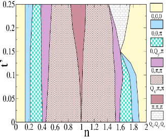
Figure 3: Colour online: The magnetic ground state in the RKKY limit, showing the dependence of the ordering wavevector ${\bf Q}$ on electron density and particle-hole asymmetry (via $t^{\prime}$). The legend for the various states is shown on the right. The calculations were done at weak coupling, $J=0.5$. Note the growing asymmetry of the phases (about $n=1$) as $t^{\prime}$ increases. It is also clear that if the hopping parameter $t^{\prime}$ changes (due to pressure, etc) the magnetic ground state can change even if the electron density remains fixed, as discussed for $4f$ systems in [20]. This is particularly prominent in the top right hand corner of the figure. In constructing this phase diagram we have ignored a narrow sliver of phase separation near $n=1$.

(iii) Intermediate coupling: The intermediate coupling regime is where one is outside the RKKY window, but not so large a coupling that only the FM and G type AFM are possible. Towards the weak coupling end it implies that the planar spirals begin to pick up a net magnetisation, $\alpha$, and now become ‘conical’ phases. Windows of phase separation also appear, particularly prominent between the $\{Q_{x},\pi,\pi\}$ and G type AFM (near $n=1$), and suggest the possibility of inhomogeneous states, etc, in the presence of disorder. The prime signature of ‘physics beyond RKKY’, however, is that the RKKY planar spirals now pick up a net magnetisation and much of the phase diagram starts to evolve towards the ferromagnetic state.

(iv) Finite temperature: The TCA based MC readily captures the FM and $\{\pi,\pi,\pi\}$ AFM phases at all coupling. However, it has difficulty in capturing the more complex spiral, A, and C type phases when we ‘cool’ from the paramagnetic phase. In the intermediate $J$ regime it usually yields a ‘glassy’ phase with the structure factor having weight distributed over all ${\bf q}$. In our undertstanding this is a limitation of the small cluster based TCA, and the energies yielded by VC are better than that of ‘unordered’ states obtained via MC. To get a feel for the ordering temperature we have calculated the energy difference $\Delta{\cal E}$, defined earlier, as often done in electronic structure calculations. This provides the trend in $T_{c}$ across the phases, Fig.2, and wherever possible we have included data about actual $T_{c}$ (symbols) obtained from the MC calculation. Broadly, with increasing $J$ the $\Delta{\cal E}$ and $T_{c}$ scales increase but the number of phases decrease. The $T_{c}$ of the G type AFM is expected to fall at large $J$ but even at $J/t=10$ it is larger than the peak FM $T_{c}$.

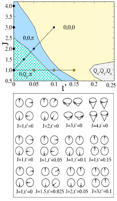
Figure 4: Colour online: Top: the magnetic ground state at $n=1.7$ for varying $t^{\prime}$ and $J$. The ordering wavevector is marked on the phases. The magnetic order has a pronounced dependence on both the ‘bandstructure’ (through $t^{\prime}$) and the electron-spin coupling. We highlight three kinds of parameter variation. (i) Varying $J$ at fixed $t^{\prime}$, the points on the $y$ axis, shows how changing electron-spin coupling can change the ground state. (ii) Varying $t^{\prime}$ at weak coupling, $J=1$, illustrates how bandstructure affects the RKKY magnetic order. (iii) In the $4f$ elements we think what happens is a combination of (i) and (ii) above, as shown by points on the diagonal. Bottom: An impression of the real space spin configuration for the three parameter sets (i)-(iii) in the top panel. Each $2\times 2$ pattern is for a $t^{\prime},~{}J$ combination. The bottom left spin in each pattern is set on the reference site ${\bf R}=\{0,0\}$, say. The neighbouring three spins are at $\{{\hat{x}},0\}$, $\{0,{\hat{y}}\}$, and at $\{{\hat{x}},{\hat{y}}\}$, where ${\hat{x}}$ and ${\hat{y}}$ are unit vectors on the lattice. There is no variation in the $z$ direction so we only show the in-plane pattern. Top row: scan (i) above, changing $J$ at $t^{\prime}=0$. Middle row: scan (ii), changing $t^{\prime}$ at $J=1$. Bottom row: scan (iii), simultaneous change in $t^{\prime}$ and $J$.

(v) Interplay of FS and coupling effects: Till now we have looked at the particle-hole symmetric case where $t^{\prime}=0$. The tight-binding parametrisation of the ab initio electronic structure of any material usually requires a finite $t^{\prime}$, in addition, possibly, to multiple bands. We will use the $t-t^{\prime}$ parametrisation of band structure due to its simplicity. It will also allow us to mimic the physics in the $4f$ metals.

At weak coupling the magnetic order is controlled as usual by the band susceptibility, $\chi_{0}({\bf q},n)$ which, now, also depends on $t^{\prime}$. At fixed $n$ the magnetic order can change simply due to changes in the underlying electronic structure. Our Fig.3 illustrates this dependence, where we use $J=0.5$ to stay in the RKKY regime and explore the variation of magnetic order with $n$ and $t^{\prime}$. The range of $t^{\prime}$ variation is modest, $\sim\{0-0.3\}$, but can lead to phase changes (at fixed $n$) in some density windows. We have cross checked the phases with the peak in $\chi_{0}({\bf q})$.

A complicated and more realistic version of this has been demonstrated recently [20] in the $4f$ family for the heavy rare earths from Gd to Tm. These elements all have the same hcp crystal structure, and the same conduction electron count, $5d^{1}6s^{2}$, so nominally the same band filling. However, the electronic structure and Fermi surface changes due to variation in the lattice parameters and unit cell volume (lanthanide contraction) across the series. It has been argued [20] that this changes the location ${\bf q}_{max}$ of the peak in $\chi_{0}$, and explains the change in magnetic order from planar spiral (in Tm) to ferromagnetism in Gd. A similar effect is visible in our Fig.3 where at $n=1.7$, say, the ordering wavevector changes from a spiral to FM as $t^{\prime}$ changes from zero to $0.15$. In this scenario, $J$ does not affect the magnetic order but merely sets the scale for $T_{c}$. The RKKY interaction strength scales as $J_{eff}^{2}\sim J^{2}S(S+1)$, and a similar scaling of the experimentally measured $T_{c}$ is taken as ‘confirmation’ of the RKKY picture.

Should’nt we also worry about the effect of the growing $J_{eff}(S)$ on the magnetic order itself? If the maximum $J_{eff}$, for Gd with $S=7/2$, were smaller than the effective hopping scale $t$, then we need not - the RKKY scheme would be valid for the entire $4f$ family. However, measurements and electronic structure calculations [3] in Gd suggest that $J\sim 0.3$eV and $J_{eff}(7/2)\sim 1$eV. The effective $t$ is more ambiguous, since there are multiple bands crossing the Fermi level, but the typical value is $\sim 0.3$eV. This suggests $J_{eff}/t\sim 3$, clearly outside the RKKY window! What is the consequence for magnetic order, and physical properties as a whole?

Fig.4 shows the $t^{\prime}-J$ magnetic phase diagram at $T=0$ for $n=1.7$. At $t^{\prime}=0$, the vertical scan, changing $J$ reveals how the ordered state changes with increasing $J$ even with electronic parameters (and hence $\chi_{0}$ and FS) fixed. We have already seen this in Fig.1 The spirit of RKKY is to assume $J\rightarrow 0$, and move horizontally, changing $t^{\prime}$ across the series so that one evolves from a planar spiral to a ferromagnet. We suggest that in the $f$ metals, the parameter points are actually on a ‘diagonal’, with increasing $t^{\prime}$ (our version of changing electronic structure) being accompanied by increase in $J_{eff}$. To capture the trend we set, $t^{\prime}=0$ and $J_{eff}=1.0$ for $S=1$, where the system is known to be a spiral, and $t^{\prime}=0.1$ and $J_{eff}=3.0$ for $S=7/2$ (the case of Gd), and explore the linear variation shown in Fig.4. This parametrisation is only meant to highlight the qualitative effect of changing electronic structure and $J_{eff}$ and since real $t^{\prime}$ values, etc, would need to be calculated from an ab initio solution.

Within this framework, while the small $S$ result is same for both RKKY and explicit inclusion of $J_{eff}$, the order obtained at intermediate $S$ depends on whether one ignores $J_{eff}$ (as in RKKY) or retains its effect. For a given $t^{\prime}$ the phase on the diagonal is quite different from the phase on the horizontal line.

In fact there is evidence from earlier ab initio calculations [21] that in addition to unit cell volume and $c/a$ ratio, the strength of the $4f$ moment (and so $J_{eff}$) also affects the magnetic order. As an illustrative case, the optimal spiral wavevector in Ho evolves towards ${\bf Q}=\{0,0,0\}$ as the effective moment is (artificially) varied from $2\mu_{B}$ to $4\mu_{B}$ (Fig.2 in Nordstrom and Mavromaras [21]). If magnetism in this element, and the $4f$ family in general, were completely determined by RKKY there would be no dependence on $J_{eff}$. In fact the authors suggested that one should re-examine the basic assumptions of the ‘standard model’ of $4f$ magnetism [5], which gives primacy to the RKKY interaction (and magnetoelastic effects) since the ab initio results suggest a role for the effective exchange in the magnetic order. Our aim here has been to clarify the physics underlying such an effect within a minimal model Hamiltonian. This approach would be useful to handle non collinear phases in complex many band systems, without any weak coupling assumption, once a tight binding parametrisation of the electronic structure is available

Let us conclude. We have examined the Kondo lattice model with large $S$ spins and established the ground state all the way from the RKKY regime to the strong coupling limit. The intermediate coupling window reveals a competition between RKKY effects, which tend to generate a planar spiral, and the tendency to gain exchange energy via ferromagnetic polarisation. This generally leads to a ‘conical’ helix, giving way at strong coupling to the double exchange ferromagnet. Using these results we re-visited the classic $4f$ magnets to demonstrate how the magnetic phases there are probably controlled non RKKY spin-fermion effects. One can add anisotropies and magneto-elastic couplings to our model to construct a more comprehensive description of $4f$ magnetism.

We acknowledge use of the Beowulf cluster at HRI, and thank Sanjeev Kumar and B. P. Sekhar for collaboration on an earlier version of this problem.

References

- [1] HEWSON A. C., The Kondo Problem to Heavy Fermions, Cambridge University Press (1997).
- [2] TOKURA Y. (editor), Colossal Magnetoresistive Oxides, CRC Press (2000), CHATTERJI T. (editor), Colossal Magnetoresistive Manganites, Springer (2004).
- [3] SANTOS C., NOLTING W. and EYERT V., Phys. Rev. B 69, 214412 (2004), HEINEMANN M. and TEMMERMAN W. M., Phys. Rev. B 49, 4348 (1994).
- [4] LEGVOLD S., Ferromagnetic Materials, Vol. 1, Chap. 3., (North Holland, Amsterdam, 1980).
- [5] JENSEN J. and MACKINTOSH A. K., Rare Earth Magnetism, Clarendon, Oxford (1991).
- [6] ELLIOTT R. J., Phys. Rev. 124, 346 (1961).
- [7] For an overview see, JUNGWIRTH T., SINOVA J., MASEK J., KUCERA J., and MACDONALD A. H., Rev. Mod. Phys. 78, 809 (2006).
- [8] RUDERMAN M. A., and KITTEL C., Phys. Rev. 96, 99 (1954), KASUYA T., Prog. Theor. Phys. 16, 45 (1956), YOSIDA K., Phys. Rev. 106, 893 (1957).
- [9] ZENER C., Phys. Rev. 82, 403 (1951), ANDERSON P. W., and HASEGAWA H., ibid. 100, 675 (1955), de GENNES P-G., ibid. 118, 141 (1960).
- [10] CALDERON M. J. and BREY L., Phys. Rev. B 58, 3286 (1998), MOTOME Y. and FURUKAWA N., J. Phys. Soc. Jpn. 69 (2000) 3785.
- [11] PEKKER D., MUKHOPADHYAY S., TRIVEDI N., and GOLDBART P. M, Phys. Rev. B 72, 075118 (2005).
- [12] CHATTOPADHYAY A., MILLIS A. J. and DAS SARMA S., Phys. Rev. B 64, 012416 (2001).
- [13] KIENERT J., et al., Phys. Rev. B 73, 224405 (2006).
- [14] DAGOTTO E., YUNOKI S., MALVEZZI A. L., MOREO A., Hu J., CAPPONI S., POILBLANC D., FURUKAWA N., Phys Rev B 58 6414 (1998).
- [15] KUMAR S., and MAJUMDAR P., Eur. Phys. J. B 46.
- [16] For examples of variational calculations, see HAMADA M., and SHIMAHARA H., Phys. Rev. B 51, 3027 (1995), ALONSO J. L., CAPITAN J. A., FERNANDEZ L. A., GUINEA F., and MARTIN MAYOR V., Phys. Rev. B 64, 054408 (2001).
- [17] KUMAR S. and MAJUMDAR P., Eur. Phys. J. B 50, 571 (2006).
- [18] Our choice corresponds to a periodically varying azimuthal angle, . The most general periodic state involves periodic variation in the polar angle as well [16].
- [19] PRADHAN K. and MAJUMDAR P., to be published.
- [20] HUGHES I. D., DANE M., ERNST A., HERGERT W., LUDERS M., POULTER J., STAUNTON J. B., SVANE A., SZOTEK Z., TEMMERMAN W. M., Nature, 446, 650 (2007).
- [21] NORDSTROM L. and MAVROMARAS A., Europhys. Lett. 49, 775 (2000).