We solve numerically the equations of nonlinear fluctuating hydrodynamics (NFH) for the supercooled liquid. The time correlation of the density fluctuations in equilibrium obtained here shows quantitative agreement with molecular dynamics(MD) simulation data. We demonstrate numerically that the $1/\rho$ nonlinearity in the NFH equations of motion is essential in restoring the ergodic behavior in the liquid. Under nonequilibrium conditions the time correlation functions relax in a manner similar to that observed in the molecular dynamics simulations in binary mixtures. The waiting time $t_{\mathrm{w}}$ dependence of the non-equilibrium response function follows a Modified Kohlrausch-Williams-Watts(MKWW) form similar to the behavior seen in dielectric relaxation data.

Time dependent correlations in a supercooled liquid from nonlinear fluctuating hydrodynamics.

The conserved densities of mass, momentum, and energy constitute the simplest set of slow modes characteristic of the isotropic liquid. The microscopic balance equations for the respective conservation laws contain terms with widely different characteristic time scales of variation respectively corresponding to the various degrees of freedom of the complex system. The nonlinear fluctuating hydrodynamics (NFH) describes the dynamics of these slow modes with nonlinear differential equations having regular and stochastic parts. The regular parts involve nonlinear coupling of slow modes while the random parts represent noise which can be linearDM ; ABL ; hayakawa or multiplicativeABL ; kim-kawasaki . The most widely studied theoretical model for the slow dynamics in a supercooled liquid approaching vitrification follows from these equations of NFH and is termed as the self-consistent mode coupling theory (MCT) rmp ; reichman . In a strongly interacting dense liquid the coupling of density fluctuations produces the dominant effect on dynamics. The MCT involves a nonlinear feedback mechanismbeng of density fluctuations producing strong enhancement of the viscosity of the supercooled liquid. In its simplest version the MCT predicts that above a critical density the long time limit of the time correlation ${\cal C}(t)$ of density fluctuations is nonzero. This signifies an ergodic-nonergodic transition(ENE) in the liquid and is a precursor to the liquid-glass transition. The predicted dynamics involves several different regimes of relaxation and has been widely used in fitting experimental data on different liquids. However, the simple MCT approach is known to exaggerate the tendency of the dynamics towards slowing down, and becomes quantitatively inaccurate in the vicinity of the predicted transition, which is never observed in practice. The perturbation expansion for the renormalized transport coefficient in the MCT, though systematic, is in terms of a dimensionless parameter which is not small. Furthermore, it has also been shownDM ; DM1 non perturbatively that the $1/\rho$ nonlinearities in the NFH equations remove the sharp ENE transition predicted in the simplified theory. We report here the study of the slow dynamics of a dense monatomic Lennard-Jones liquid by numerically solving the stochastic equations of NFH. Our nonperturbative calculation shows good agreement with the computer simulation results of the same system in equilibrium. We also report here results on the dynamics of the density fluctuations under nonequilibrium conditions.

We consider the equations of NFH for an isotropic liquid in its simplest form for the mass density $\rho$ and momentum density gDM

$$\frac{\partial\rho}{\partial{t}}+{\bf\nabla}.{\bf g}=0,$$ (1)

$$\frac{\partial g_{i}}{\partial t}+\nabla_{j}\left[\frac{g_{i}g_{j}}{\rho}\right]+\rho\nabla_{i}\frac{\delta F_{U}}{\delta\rho}+L_{ij}\frac{g_{j}}{\rho}=\theta_{i}~{}~{}.$$ (2)

The correlations of the gaussian noise $\theta_{i}$ are related to the bare damping matrix $L_{ij}$ hansen , $\left\langle\theta_{i}(x,t)\theta_{j}({x^{\prime}}t^{\prime})\right\rangle=2k_{B}TL_{ij}\delta(t-t^{\prime})\delta(x-x^{\prime})$. For an isotropic liquid, $L_{ij}=(\zeta_{0}+\eta_{0}/3)\delta_{ij}\nabla^{2}+\eta_{0}\nabla_{i}\nabla_{j}$ where $\zeta_{0}$ and $\eta_{0}$ respectively denote is the bare bulk and shear viscosities. The stationary solution to the Fokker-Planck equation corresponding to the generalized Langevin eqn. (2) is obtained as $\exp\{-\beta{F[\rho,g]}\}$ with $\beta=1/{k_{B}T}$ is the Boltzmann factor. The coarse grained free energy functional is obtained as $F[\rho,g]\equiv F_{K}[\rho,g]+F_{U}$. The kinetic part is dependent on the momentum density $F_{K}=\int d{\bf x}g^{2}/(2\rho)$ and the so called potential part is given by $F_{U}=F_{\mathrm{id}}+F_{\mathrm{int}}$. The ideal gas contribution is $F_{\mathrm{id}}=\int d{\bf r}\rho({\bf r})[\ln(\rho({\bf r})/\rho_{0})-1]$. The interaction part $F_{\mathrm{int}}$ up to quadratic order in density fluctuationstvr is obtained as

$$\beta F_{\mathrm{int}}=-\frac{1}{2m^{2}}\int d{\bf r}d{\bf r}^{{}^{\prime}}c(\textbf{r}-\textbf{r}^{{}^{\prime}})\delta\rho(\textbf{r})\delta\rho(\textbf{r}^{{}^{\prime}})~{}~{},$$ (3)

where $c(r)$ is the two point Ornstein-Zernike direct correlation functionhansen and $m$ is the mass of the particles. For the glassy dynamics we focus on the coupling of slowly decaying density fluctuations present in the pressure functional, represented by the third term on the LHS of eqn. (2). With the above choice of $F_{U}$, the nonlinear contribution in this term reduces to $\rho\nabla_{i}f(r,t)$ with the convolution $f(\textbf{r},t)=m^{-1}\int d\textbf{r}c(\textbf{r}-\textbf{r}^{{}^{\prime}})\delta\rho(\textbf{r}^{{}^{\prime}},t)$.

We consider here a classical system of $N$ particles, each of mass $m$ interacting with a Lennard-Jones potential $u(r)=4\epsilon[{(\sigma/r)}^{12}-{(\sigma/r)}^{6}]$. In addition to the scale $\sigma$ of the interacting potential there is another length $h$ of the lattice grid on which $\rho$ and ${\bf g}$ are computed. We choose $\sigma/h$ to be non integer ( $=4.6$ in the present calculation) to avoid crystallization. Time is scaled with the LJ unit of $\tau_{0}=(m\sigma^{2}/\epsilon)^{\frac{1}{2}}$ and length with $h$. The thermodynamic state of the fluid is described in terms of the reduced density $n^{*}=n_{0}\sigma^{3}$ and the reduced $T^{*}=(k_{B}T)/\epsilon$. For numerical solution the conserved densities are scaled to dimensionless forms: $n(\textbf{r})=[h^{3}m^{-1}]\rho(\textbf{r})$, and $\textbf{j}(\textbf{r})=[h^{3}(m\epsilon)^{-\frac{1}{2}}]\textbf{g}(\textbf{r})$. The speed of sound $c_{0}$ is given by, $c_{0}^{2}=k_{B}T/(mS(0))$. We start with an initial distribution of the fluctuating variables $n(\textbf{r})$ and $\textbf{j}(\textbf{r})$ over a set of points $20^{3}$ on a cubic lattice. The nonlocal integral $f(r,t)$ is evaluated as a sum of contributions from the successive shells, $f(r,t)=h^{3}\sum_{i}c(R_{i})\sum_{\alpha}\delta n(R_{i}^{\alpha},t)$, where $R_{i}^{\alpha}$ for $\alpha=1,...m_{i}$ respectively denote radii vectors of the $m_{i}$ lattice points in the ith spherical shell of radius $R_{i}$. The $1/\rho$ nonlinearity in the dissipative term of the momentum equation is computed by replacing the density field in the denominator with the $\rho({\bf x})$ averaged over a length scale close to $\sigma$ around the corresponding point ${\bf r}$. We ignore the convective nonlinearity in the present calculation and focus on the role of the pressure nonlinearity in producing the slow dynamics.

A major hurdle encountered in the numerical scheme used here arises from an instability which occurs as $n({\bf x},t)$ gets negative at certain grid points. To avoid this situation, we redefine $n({\bf x},t)$ on the grid at each step of the numerical integration with a coarse graining scheme. In devising the latter we make use of the following physical interpretation of the definition of $\rho({\bf x},t)$ of the density field : the integral $\int_{\Delta{V}}d{\bf x}\rho({\bf x},t)$ represents the total mass in an elementary volume $\Delta{V}$ of the system. At each time step of the numerical integration, the positivity of the field $n({\bf x})$ over the whole grid is checked. If it turns negative at a point, we reduce $n({\bf x})$ at some or all of the neighboring sites by taking equal contributions from each and add the sum total to the original site. It is also ensured that the density at none of the neighboring sites becomes negative as a result of this redistribution. The sum of the densities at the original and the contributing sites remains unaltered and hence global conservation is maintained. If the above redistribution involving contributions only from the nearest neighbor sites is insufficient to make $n({\bf x})$ positive everywhere, we include the next nearest neighbors in the redistribution and so on. In reality however we hardly need to include beyond the second shell of neighbors surrounding the original site. With the density instability being corrected with this coarse graining procedure, the numerical algorithm can be run up to much larger times than in earlier worksdasgupta . The arbitrary regularization of the strength of the noise dasgupta can also be avoided, and the fluctuation dissipation relation respected.

The equal-time correlation of density fluctuations for the $N$ particle system is given by $S(k,t)={N}^{-1}<\delta n(k,t)\delta n(-k,t)>$ where the angular brackets refer to an average over the noise. We first consider the system as it evolves at $T^{*}=2.0$ and $n_{0}^{*}=.97$ under the influence of thermal noise, starting from an initial state in which all fluctuations are set to zero. Time translational invariance is reached as the system equilibrates and $S(k,t)$ approaches the corresponding static structure factor $S(k)$. The equilibrated $S(k)$ vs. $k$ plot ( for large $t_{\mathrm{w}}$ ) is displayed in fig. 1. $S(k,t)$ obtained with equations of motion linear in fluctuations is also displayed. The peak position ($q_{m}$) and amplitude of the $S(k)$ obtained ( using the Ornstein-Zernike relation) from the input direct correlation function $c(r)$ are well reproduced. Other features of $S(k)$ are partly lost due to the relatively crude grid size used in our numerical solution.

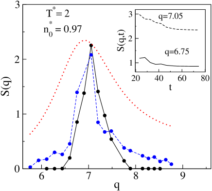
Figure 1: $S(k)$ vs $k\sigma$ at $T^{*}=2$ and $n_{0}^{*}=0.97$ for linear (solid) and nonlinear (dashed) dynamics; as computed from input $c(r)$ (dotted). Inset: $S(k,t)$ vs $t$ for $k\sigma=6.75$ (solid) and $k=7.05$ (dashed) displaying equilibration with time.

Next we focus on the dynamic correlation function ${C}(t+t_{\mathrm{w}},t_{\mathrm{w}})$ defined in the normalized form ${C}(t+t_{\mathrm{w}},t_{\mathrm{w}})={<\delta n(t+t_{\mathrm{w}})\delta n(t_{\mathrm{w}})>}/{<\delta n(t_{\mathrm{w}})\delta n(t_{\mathrm{w}})>}.$ For large $t_{\mathrm{w}}$ time translational invariance holds, making ${C}(t+t_{\mathrm{w}},t_{\mathrm{w}})\equiv{\cal C}(t)$. The decay of ${\cal C}(q_{m},t)$ is compared in fig. 2 with the corresponding molecular dynamics simulation resultsullo for the equilibrated systems at $T=.6$ for two densities $n_{0}^{*}=1.10$ and $n_{0}^{*}=1.06$. The input $c(r)$ corresponds to the purely repulsive part of the Lennard-Jones potential following Ref. ullo . The bare transport coefficients which determine the noise correlations are chosen such that the short time dynamics agrees with computer simulation results. ${\cal C}(t)$ obtained by solving the stochastic equations linearized in the fluctuations decays very fast. In comparison considerable slowing down of the decay of ${\cal C}(t)$ occurs on solving the full NFH equations. The static correlation function $S(k)$ however ( see inset of fig. 3) shows hardly any difference between the two cases. At higher densities the mean-free path of the fluid particles gets smaller and approaches the atomic length scale. As a result, the validity of Generalized hydrodynamic equations at short length scales ( corresponding to wave vector $q{\sim}q_{m}$ ) improves with increasing density. This trend is clearly seen our results displayed in fig. 2 for ${\cal C}(t)$.

The ENE transition of simple MCT is driven by the nonlinear couplings of density fluctuations in the pressure term (3rd term on LHS) of the generalized Navier-Stokes equation (2). On the other hand the $1/\rho$ nonlinearity crucial for the absence of the ENE transition is in the dissipative term of the same equation, i.e., 4th term on LHS of (2). We therefore consider two cases here to test the role of the relevant nonlinearities from a non perturbative approach. In Case A the $1/\rho$ nonlinearity in (2) is replaced with $1/\rho_{0}$ while keeping the density nonlinearity in the pressure term. In Case B, the complete model with both nonlinearities is considered. The results for ${\cal C}(q_{m},t)$ at $T=.6$ and $n_{0}^{*}=1.10$ corresponding to the Cases A and B respectively are shown in fig 3. We extend the numerical solution to the longest possible time scale ( $>10^{3}$ in Lennard-Jones units) which is about four orders of magnitude beyond the microscopic time scales. The decay of the dynamic correlation is markedly different in the two cases and agrees with the previous theoretical results on the role of $1/\rho$ nonlinearity.

To study the structural relaxation in the nonequilibrium state we consider the time evolution of the Lennard-Jones liquid following an instantaneous quench from $T^{*}_{i}=2.0$ and $n_{0}^{*}=0.97$ along the isobaric line to $T^{*}_{f}=0.4$ and $n_{0}^{*}=1.12$. We compute from the solution of the NFH equations the two-time density correlation function $C(t_{\mathrm{w}}+t,t_{\mathrm{w}})$ at $q=q_{m}$ for different waiting times $t_{\mathrm{w}}=50,$ $100,$ $200,$ $500,$ $700$ and $1000$. For small values of $t$ time translational invariance holds and $C(t_{\mathrm{w}}+t,t_{\mathrm{w}})$ depends only on $t$. On the other hand at large $t$, the correlation function depends on both $t$ and $t_{\mathrm{w}}$. Following the mean-field-theoretical resultsspin and also experimental dataexpt fits on spin glasses, we fit this long time part of the density correlation function with the form $C^{ag}\left[{h(t+t_{\mathrm{w}})}/{h(t_{\mathrm{w}})}\right]$, where $h(t)$ is a monotonously ascending function of its argument. In the $C(t_{\mathrm{w}}+t,t_{\mathrm{w}})$ vs. $[h(t+t_{\mathrm{w}})/h(t_{\mathrm{w}})]^{\alpha}$ plot, the parameter $\alpha$ is tuned to obtain a collapse of all the curves. The results displayed in the fig. 4 obtain $h(t)\sim[\rm{log}(t)]^{\alpha}$ with the best fit value of the parameter $\alpha=.81$. This is comparable to the corresponding value $\alpha=.88$ obtained in molecular dynamics simulations KB of binary Lennard-Jones mixtures.

In a recent work, Lunkenheimer et. al. loidl studied over a range of frequency $\omega$ the dielectric response function $\chi_{\omega}(t_{\mathrm{w}})$ at temperature $T<T_{g}$. The system falls out of equilibrium over laboratory time scales at the calorimetric glass transition temperature $T_{g}$. The aging time ($\equiv{t_{\mathrm{w}}}$ in the present notation) dependence of $\chi$ follows a modified Kohlrausch-Williams-Watts (MKWW) function $\tilde{f}(t_{\mathrm{w}})=\exp[{(t_{\mathrm{w}}/\tau(t_{\mathrm{w}}))}^{\bar{\beta}}]$. The relaxation time $\tau(t_{\mathrm{w}})$ and the stretching exponent $\bar{\beta}$ are identical for all frequencies. The limiting value $\tau(t_{\mathrm{w}}\rightarrow\infty)$ is close to the $\alpha$-relaxation time $\tau_{\alpha}$ extrapolated to corresponding temperature $T<T_{g}$loidl . In the present work $T\sim{T_{c}}$ ($>T_{g}$) and in this case the system in fact equilibrates. We study here the function $\chi_{\omega}(t_{\mathrm{w}})=\omega C(\omega,t_{\mathrm{w}})$ which in equilibrium would reduce to the corresponding response function. $C(\omega,t_{\mathrm{w}})$ is obtained approximately (i.e. ignoring FDT violations) from the frequency transform of $C(t+t_{\mathrm{w}},t_{\mathrm{w}})$ with respect to $t$. The data is fitted to the form :

$$\chi_{\omega}(t_{\mathrm{w}})=[\chi_{\omega}^{st}-\chi_{\omega}^{eq}]\tilde{f}(t_{\mathrm{w}})+\chi_{\omega}^{eq},$$ (4)

where $\chi_{\omega}^{st}$ and $\chi_{\omega}^{eq}$ respectively refer to the initial and final values of $\chi_{\omega}$. For the relaxation time in $\tilde{f}$ we usesen_das $\tau(t_{\mathrm{w}})=\left(\tau_{\mathrm{st}}-\tau_{\mathrm{eq}}\right)f(t_{\mathrm{w}})+\tau_{\mathrm{eq}}$ with the normalized function $f(t)=2^{\bar{\beta}}/{[1+\exp\{2t/\tau(t)\}]}^{\bar{\beta}}$. Fig. 5 shows that $\chi_{\omega}$’s at different frequencies scale onto a single master curve for $\beta=0.68$. The $\tau(t_{\mathrm{w}})$ decreases sharply with $t_{\mathrm{w}}$ initially and becomes almost constant at $\tau_{\mathrm{eq}}$. At large $t_{\mathrm{w}}$ the relaxation follows a stretched exponential form having the $\alpha$-relaxation time $\tau_{\mathrm{eq}}$ and exponent $\bar{\beta}$ at the corresponding temperature. This shown in the inset of fig. 5.

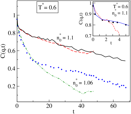
Figure 2: ${\cal C}(q,t)$ vs $t/\tau_{0}$ at $T^{*}=.6$ for densities $n_{0}^{*}=1.10$ (solid) and $1.06$ (dotted). Corresponding MD simulation dataullo shown respectively with (dashed) and (dot-dashed) curves. Inset : short time part of ${\cal C}(q,t)$ with (solid) and without (dashed) nonlinear coupling of modes; corresponding MD simulation resultullo (dark circles).

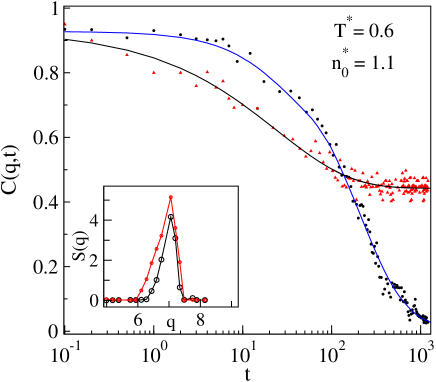
Figure 3: ${\cal C}(q,t)$ vs $t/\tau_{0}$ at $T^{*}=.6$ and $n_{0}^{*}=1.10$ for case A (filled circles) and case B (filled triangles). The solid lines are the best fit curves to the corresponding data. Inset : $S(k)$ vs $k\sigma$ for the two cases respectively with solid and dashed curves.

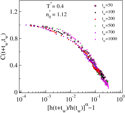
Figure 4: Normalized correlation function $C(t_{\mathrm{w}}+t,t_{\mathrm{w}})$ vs. ${[h(t+t_{\mathrm{w}})/h(t_{\mathrm{w}})]}^{\alpha}$ for different waiting times $t_{\mathrm{w}}/\tau_{0}$ shown in the inset . The data at large $t$ scales onto a single master curve with $h(t)\sim\log(t)$ and $\alpha=.81$.

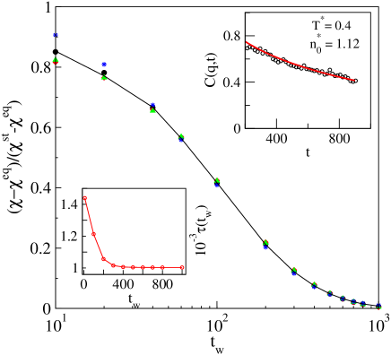
Figure 5: Scaling of $\chi_{\omega}(t_{\mathrm{w}})$ for frequencies $\omega\tau_{0}$ = $10^{-2}$(circle), $10^{-1}$(diamond), $10^{0}$ (triangle), and $10^{1}$ (star). solid line is a fit to MKWW form. Lower inset : $\tau(t_{\mathrm{w}})$ vs $t_{\mathrm{w}}/\tau_{0}$. Upper inset : ${\cal C}(q_{m},t)$ vs $t/\tau_{0}$ at the final state $T^{*}=0.4$ and $n_{0}^{*}=1.10$ (circles); solid line is fit to a KWW form with exponent $\bar{\beta}=0.68$ and relaxation time $\tau_{eq}$(see text).

We have shown that the direct numerical solutions of the NFH equations provide a reliable way of studying the dynamics of fluctuations in a dense liquid in the vicinity of the avoided ergodic nonergodic transition. While the method is not appreciably more efficient than molecular dynamics from a computational standpoint, it provides an interesting way of investigating theoretical assumptions that can be made in the analytical treatment of these equations. In particular, our work clearly shows the role of the $1/\rho$ nonlinearity present in the dissipative term of eqn. (2) in restoring ergodicity DM . The present method can be easily extended to a larger set of hydrodynamic variables, which would permit a description of the dynamics in binary mixtures. For the nonequilibrium states, the dynamics with the one loop mode coupling theory has been formulated for the spherical p-spin glass modelkurchan . For the supercooled liquid a similar analysis even at the one loop level is still lacking. Our numerical approach is by essence non perturbative, and it will be interesting to compare it to analytical perturbative approaches to the same equations under nonequilibrium conditions. The CEFIPRA is acknowledged for financial support under Indo-French research project 2604-2.

References

- (1) S. P. Das and G. F. Mazenko, Phys. Rev. A, 34, 2265 (1986).
- (2) A. Andreanov, G. Biroli, and A. Lefevre, J. Stat. Mech, PO7008 (2006).
- (3) T. N. Nishino and H. Hayakawa, Cond-mat. 0803.1797v2
- (4) B. Kim and K. Kawasaki, J. Stat. Mech, P02004 (2008).
- (5) S. P. Das, Rev. of Mod. Phys. Rev. 76, 785 (2004).
- (6) D. R. Reichman and P. Charbonneau, J. Stat. Mech., P05013 (2005).
- (7) U. Bengtzelius, W. Götze and A. Sjölander, 1984, J. Phys. C 17, 5915.
- (8) S. P. Das and G. F. Mazenko, Cond-mat 0801.1727.
- (9) J-P. Hansen and I.R. . McDonald, Theory of Simple Liquids, 3rd ed. Academic, London (2006).
- (10) T. V. Ramakrishnan and M. Yussouff, Phys. Rev. B. 19, 2775 (1979).
- (11) L. M. Lust, O. T. Valls and C. Dasgupta, Phys. Rev E. 48, 1787 (1993); O. T. Valls and G. F. Mazenko, Phys. Rev A. 46, 7756 (1992).
- (12) J. J. Ullo and S. Yip, Phys. Rev. Lett 54, 1509 (1985)
- (13) J.-P. Bouchaud, L. F. Cugliandolo, J. Kurchan, and M. Mezard, Physica (Amsterdam) 226A, 243 (1996).
- (14) H. Rieger, J. Phys. A 26, L615 (1993).
- (15) W. Kob and J. L. Barrat, Phys. Rev. Lett. 78, 4581 (1997).
- (16) P. Lunkenheimer, R. Wehn, U. Schneider, and A. Loidl, Phys. Rev. Lett. 95, 055702 (2005).
- (17) B. Sengupta and S. P. Das, Phys. Rev. E, 76, 061502 (2007).
- (18) L. F. Cugliandolo and J. Kurchan, Phys. Rev. Lett. 71, 173 (1993).