Finite size effect of harmonic measure estimation in a DLA model: variable size of probe particles

Abstract

A finite size effect in the probing of the harmonic measure in simulation of diffusion-limited aggregation (DLA) growth is investigated. We introduce variable size of the probe particles to estimate harmonic measure and extract fractal dimension of DLA clusters taking two limits, of vanishingly small probe particle size and of infinitely large size of a DLA cluster. We generate 1000 DLA clusters consisting of 50 million particles each using off-lattice killing-free algorithm developed in the early work. The introduced method leads to an unprecedented accuracy in the estimation of the fractal dimension. We discuss the variation of the probability distribution function with the size of probing particles.

I Introduction

There is a wealth of processes and systems ranging from the crystal growth and dendrites formation to bacteria colonies growth and dielectric discharge patterns (see BH for a review) that evolve in time in a similar manner following a generic process called the two dimensional aggregate growth. The specific model which is a most common representation of this process is the diffusion limited aggregation (DLA) WS and its generalization, dielectric breakdown model (DBM) Pietronero capturing most of the dynamic properties of the random aggregates evolution BH . While analytical and numerical studies have had impressively advanced our understanding of the DLA BH ; TH-review , several critical issues remain unresolved. One of the major controversies is related to the multiscale and fractal nature of DLA. It has been a common belief that DLA, DBM and Laplacian growth Saffman58 belong to the same universality class. Recently, however, this common wisdom was questioned in Ref. Barra2001 ; Hentschel2002 , where it was argued that DLA and Laplacian growths have different fractal dimensions. To resolve this intriguing issue a breakthrough in the precision of the data on fractal dimensions of both models is required. In our work we will address the algorithms and techniques that offer a dramatic improvement in determining the DLA fractal dimension $D$ characterizing DLA clusters.

The DLA/DBM models and growth algorithms are based on the aggregation of the particles randomly diffusing in the plane. A noticeable progress was made owing to the technique introduced recently by Hastings and Levitov HL where the electric field equations appearing in DBM were solved by iterative conformal mapping, and freely diffusing particles could reach any given site of the surface. The approach of HL was further extended by Hastings Hastings02 where the models of the Laplacian Random Walk (LRW) similar to DLA, with the exception that the growth occurs only at the tip, were proposed. In the continuum limit this model transforms into the stochastic Loewner evolution (SLE) SLE ; Cardy-SLE-rev . Yet, within the conformal mapping techniques fairly large clusters are to be built to insure a reasonable precision in determining the fractal dimensionality because the relative fluctuations decrease very slow with the cluster size. Namely, squared relative fluctuations

$${\cal F}_{D}{=}\left(\langle D^{2}\rangle{-}\langle D\rangle^{2}\right){/}\langle D\rangle^{2}$$ (1)

scale as $N^{-0.33}$ with the cluster size $N$ RS ; DLA-MS . This is caused by large deviations in the cluster structure across the ensemble: each cluster has its own particular shape and preferred directions; these shapes vary in time and do not converge to any common “typical” structure.

Random aggregate growth is fully characterized by the harmonic measure, i.e. by the probability for the surface to advance at some given segment. A common recipe for measuring this probability in computer experiments was to use the probe particles of the same size as particles that comprise the aggregate. To count the controversies concerning the issue of the universality of random aggregate growth, we undertake more precise analysis of DLA model, based on the probing particles of variable size. As it was shown DLA-MSV , this technique can significantly increase the accuracy of the fractal dimension estimation. We build the ensemble of 1000 DLA clusters, 50 millions particles each, generated by the off-lattice killing-free algorithm DLA-MS which we now modify to insure the free zone tracking. By using probe particles of different size $\delta$ and then taking the limit $D(\delta,N),\delta\rightarrow 0$ we find fractal dimension measured on the whole surface including also the regions that were inaccessible to the probe particles of the fixed size. Another important feature of our approach, is that the small particles are more sensitive to the fjords, while the large particles feel better the tips of the cluster. Thus, using the variable size-particles we measure not only the influence of the active growing zones (the hot part of the cluster) but also the effect of the “accomplished” (frozen, or cold) parts of the cluster. As a result, the large fluctuations of the fractal dimension $D(\delta,N)$ are suppressed. Taking then the second limit $D=D(N),N\rightarrow\infty$ we find DLA-MSV that $D$ converges to the value of $D=1.7100(2)$ which is the order of magnitude improvement as compared to past simulations.

The paper is organized as follows. In section II we give details of the off-lattice killing-free algorithm we use to generate clusters and of the procedure of estimation of DLA fractal dimension. Section III contains brief discussion of the dependence of fractal dimension from the cluster size and section IV discusses walk of the center of cluster mass as cluster grows, and the two ways to calculate cluster radii - as distance from origin and as distance from center of mass. Section V describes the original method of fractal dimension estimation with the additional parameter, the size of the probe particles. We discuss in section VI how the probability distribution function for particle to stick cluster at the distance $r$ varies with the size of the probe particles. Finally, in the section VII we discuss our results and possible future developments.

II Simulations

II.1 DLA algorithm

The original DLA algorithm WS starts with placing a seed particle at the origin of a square lattice. Than at certain position, far away from the seed, a new particle is released, which wonders stochastically over the lattice until it runs into and sticks to the seed particle. If in the course of random walk a particle crosses the lattice boundary it gets removed (killed). A new particle is generated and process repeats. Successive aggregation of particles forms a DLA cluster. Several improvements to this original algorithm were developed in order to speed up the simulations  BB-alg ; TM-alg . Later it was found that large cluster exhibit anisotropy which reflects the symmetry of the lattice MBRS-alg .

There exist also the off-lattice versions of the same algorithm. Namely, the particles are assumed to be balls that move freely in each direction. Making use the off-lattice algorithm one can easily speed up simulations by utilizing improvements introduced in BB-alg ; TM-alg ; KVMW ; SSZ ; book , in particular, the large step sizes, returns instead of killing, etc.

Another algorithm for generating the DLA-like cluster is the well-known DBM model Pietronero . Instead of tracing the motion of particles, one solves a Laplace equation and calculates a probability for a particle to hit the surface at the given site. Adding particles successively with the calculated probability, one generates a DBM cluster.

II.2 Off-lattice killing-free algorithm

We utilize the realization of the off-lattice killing-free algorithm described in DLA-MS , in which we upgraded the free-zone calculation. An essential feature of our algorithm, that it is a memory saving one; the memory organization is similar to that used in the Ball and Brady algorithm BB-alg . The modifications we have introduced are as follows: (i) we employ the large walk steps; (ii) we use a killing-free rule for exact evaluating the probability for the particle to return at the birth circle; (iii) we use only two layers in the memory hierarchy; (iv) we use a recursive algorithm for the free zone tracking; and (v) the size of free zone is calculated precisely for the particles moving near the cluster boundary. Our further improvement of the walk procedure [item (iv) above] is that instead of performing the search of free cells each time particle is moving, we pass all the cells and recalculate the free-zone sizes after the addition of each particle.

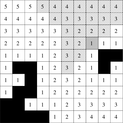
Figure 1: Occupied lattice sites and sizes of free zones around each cell. The gray cell is the newly occupied one. Shaded cells are cells where free zone size will be recalculated.

The killing-free algorithm consists of the following steps: 1) Placing a seed particle at the origin (0,0). 2) Generating a new particle at a random position on $R_{b}$. 3) Moving the new particle by fixed steps in random directions. 4) Aggregating a particle to the cluster in case it collides with either the seed or the cluster itself. 5) Generating a new particle position on $R_{b}$ with the probability

$$P(\delta\phi)=\frac{1}{2\pi}\frac{1-x^{2}}{x^{2}-2x\cos{\delta\phi}+1},$$

where $x=r/R_{b}$ and $\delta\phi$ is the change in particle angle, in case where the particle falls into a dead circle $R_{d}$, $R_{d}>R_{b}$. 6) Repeating the cycle from the step 2.

Since particles are moving randomly in the plane and assuming that the step size is negligible as compared to the dimension of the free zones around a particle (unless it gets close to the cluster), one could speed up the computational process by increasing the step size. This requires reliable and efficient identification of such “cluster free” regions. The common approach is to use the hierarchical memory model and store particles into cells, which will comprise the first layer. The second layer consists of cells which are several times larger than those at the first layer, and so on. Starting with the largest-scale cells layer, one checks their occupancy until the unoccupied cell is found. If the process is successful one gets the size of free zone at ones. Unfortunately, for the large enough clusters this approach is memory consuming and inefficient, because of the high degree of the granularity.

We use a double layer memory organization: Particles are stored in the square cells, the latter also describe the size of free area around them. This information is updated during the attaching a new particle. Let $i,j$ be the indexes of some cell on the lattice and $x_{n},y_{n}$ be the indexes of some occupied cell. Then the free zone around the $i,j$ cell is $d_{i,j}=\min_{n}{max(|i-x_{n}|,|j-y_{n}|)}$ where the $\min$ is taken over all occupied cells. Figure 1 shows the lattice where occupied cells are black and numbers denote the free area sizes around each empty cell. As a new cell gets occupied (marked grey in the Figure) one has to check all the cells around it and recalculate $d_{i,j}$. Shaded cells on the picture are those where the distances are going to be changed. One can see that the perturbation propagates continuously – all the shaded cells are connected with each other. This continuous propagation holds for every configuration of cells.

In order to track down all the cells where the distances have changed, one should traverse first all the adjacent cells around the new one (grey cell in the Figure), then the next nearest cells that have changed the neighbors and so on. Since this process is unrestricted in time and can continue indefinitely (corresponding to the upward propagation in the figure), we stop the process after having spanned the distance of 15 and assume that cells where distance is not specified have free zone sizes of 15 as well.

For large clusters the cavities between the branches become bigger than 15 cell sizes. In order to overcome this limitation we use the two layer memory model each having free zone size counters updated by the rules we have described above. For clusters of size 50 million particles we choose first layer cell size of 32 and second layer - 128, and the particle radius is unity.

On the close distance to the cluster we found useful to find precise distance to the cluster by iterating over all adjacent particles. This step is only required when current cell is marked as occupied or is adjacent to the occupied one and big step based on coarse grain information given by free/occupied cells is not enough.

All these improvements of DLA realization algorithm enable us to generate each cluster with 50 million particles in about 3 hours on 3Ghz Pentium 4 with 2 GB of RAM.

II.3 Fractal dimension estimation

The fractal dimension of a random aggregate is the quantity $D$ defined by the scaling relation

$$R\propto N^{1/D},$$ (2)

where $R$ is a linear measure of the cluster consisting of $N$ particles. Several possible choices of the characteristic length $R$ are listed in Table 1.

II.3.1 Ensemble averaging

Let $M$ denote the number of clusters we have generated and $r_{N}(k)$ be the position of the $N$-th particle in the $k$-th aggregate. Then the deposition radius is

$$R_{\rm dep}(N)=\langle r_{N}\rangle=\frac{1}{M}\sum_{k=1}^{M}r_{N}(k).$$

Other quantities we are interested in are the gyration radius, $R_{\rm gyr}$, the root mean squared (RMS) radius $R_{2}$, and the penetration depth $\xi$, with the definitions given in the upper part of the Table 1.

In order to understand the behavior of the fractal dimension in the limit of infinite clusters one can check the dependence of $D$ versus $N$. We extract $D(N_{0})$ as the result of fitting some $R$ to the scaling relation (2) when $N$ varies from 0 to $N_{0}$ or in other words using clusters of size less than $N_{0}$.

II.3.2 Harmonic measure averaging

Harmonic measure is defined on the surface of the cluster as the probability of the DLA cluster to grow at the given point. One can define the deposition radius as $R_{\rm dep}^{hm}=\int rdq$, where the integral is taken over the cluster surface and $dq$ is the growth probability at point $r$. Using this harmonic measure we calculate fractal dimension of $k$-th cluster $D_{k}(N)$, and perform averaging over the ensemble of clusters, $D(N)=\frac{1}{M}\sum_{k=1}^{M}D_{k}(N)$.

In simulations we estimate harmonic measure averages in the following way. We use probe particles which move due to the convention rules but do not stick to the cluster. Instead we track the position $r_{i}$ where $i$-th particle hits the cluster. Then deposition radius $R_{\rm dep}^{hm}$ estimated as average $R_{\rm dep}^{hm}=\frac{1}{N_{p}}\sum_{i=1}^{i=N_{p}}r_{i}$. Calculating harmonic-measure averages is very time consuming procedure. The number of probe particles $N_{p}$ used is chosen dynamically so that relative error of $R_{\rm dep}^{hm}$ is less than 0.001. See the lower part of Table 1 for the definitions used.

Ensemble averages
	Length	Definition	$D$
Deposition radius	$R_{\rm dep}$	$\langle r\rangle$	$1.71111(59)$
RMS radius	$R_{2}$	$\sqrt{\langle r^{2}\rangle}$	$1.71155(29)$
Gyration radius	$R_{\rm gyr}$	$\sqrt{\frac{1}{N}\sum_{k=1}^{N}\langle r^{2}\rangle_{k}}$	$1.71149(30)$
Penetration depth	$\xi$	$\sqrt{{R_{2}}^{2}-{R_{\rm dep}}^{2}}$	$1.7184(65)$
Harmonic measure averages
Deposition radius	$R_{\rm dep}^{hm}$	$\int r\,{d}q$	$1.70922(97)$
RMS radius	$R_{2}^{hm}$	$\sqrt{\int r^{2}\,{d}q}$	$1.70944(87)$
Effective radius	$R_{\rm eff}^{hm}$	$\exp{(\int\ln r\,{d}q)}$	$1.70944(87)$
Penetration depth	$\xi^{hm}$	${R_{2}^{hm}}^{2}-{R_{\rm dep}^{hm}}^{2}$	$1.74(3)$

Table 1: Estimates of the fractal dimension $D$ extracted with the fit $N\propto R^{D}$ to the dependence of the various lengths with ensemble size of 1000 clusters each with $5\cdot 10^{7}$ particles.

III Oscillations of fractal dimension with the cluster size and weak self-averaging

One can expect that the fractal dimension can be found as the limit $D(N)$, as $N\rightarrow\infty$. Unfortunately, this simple approach fails because of the non-monotonic $D(N)$ dependence with the rather large variations in $D(N)$ DLA-MS .

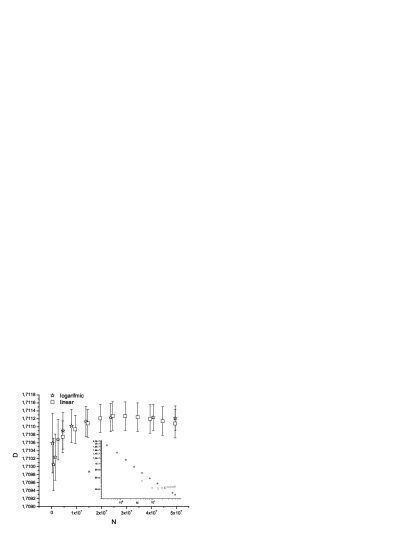
Figure 2: Fractal dimension as function of $N$ measured with $R_{\rm dep}^{hm}$ and harmonic measure averaging over 100 clusters of size $5\cdot 10^{7}$. Stars represent estimation in logarithmic scale, and boxes - in linear scale. In the inset: dependence of relative squared fluctuations of $D$ with $N$.

We measure fractal dimension for each cluster using $R_{\rm dep}^{hm}$ and then we calculate the ensemble average of fractal dimension and its variation. There are two ways of extracting $D$ from the $R(N)$ dependence: either via choosing points in $R_{\rm dep}^{hm}$ curve to be uniform on either the linear scale, or on the logarithmic one. It seems that both procedures result in the same average value of $D$, but exhibit different behaviors of the variances, see Figure 2. If points are distributed uniformly in the logarithmic scale, then $\cal F_{D}$ (1) changes as $N^{-0.33}$ as was found previously in our paper DLA-MS . In contrast, $D$ measured by the points uniformly distributed on the linear scale shows larger fluctuations without any visible decay with $N$.

One can try to understand this behavior as follows. Varying points distribution we, accordingly, change their respective weights. If points are uniform on the linear scale, then $D$ is more sensitive to the behavior of the bigger clusters, and the error when determining $D$ does not change with the size of the cluster very much. One can say that $D$ exhibits the lack of self-averaging in this case. On the contrary, the uniformity on the log scale gives rise to a weak self-averaging of $D$.

The two procedures both yield very close values of $D$ as one can check in Figure 2, therefore for the rest of this paper we will use the points uniformity on the linear scale because this choice requires less CPU time for calculating the harmonic measure.

IV Center of mass fluctuations

Each realization of a DLA cluster is a unique object: its branch structure varies very much from sample to sample. This causes large fluctuations in cluster properties and reflects in the behavior of the center-of-mass position of a cluster. At any moment of time (which is proportional to the number of particles in the cluster $N$) there are some preferred directions of growth. These directions vary in time as illustrated in Figure 3, where we present the variations of the center-of-mass positions in plane coordinates $(X,Y)$ for five different clusters. The center-of-mass positions (CoM) for each cluster are marked with their own symbol (circles, rhombi, triangles, stars, and boxes). Each mark placed after $2\cdot 10^{6}$ particles were added, so the history of the center-of-mass variation represents the time from $10^{5}$ to $5\cdot 10^{7}$. One sees from Figure 3, that for some clusters (marked with stars), position of the CoM is mainly rotated around the origin, while for some of them (marked with boxes) CoM is diffused from the origin in the given time interval.

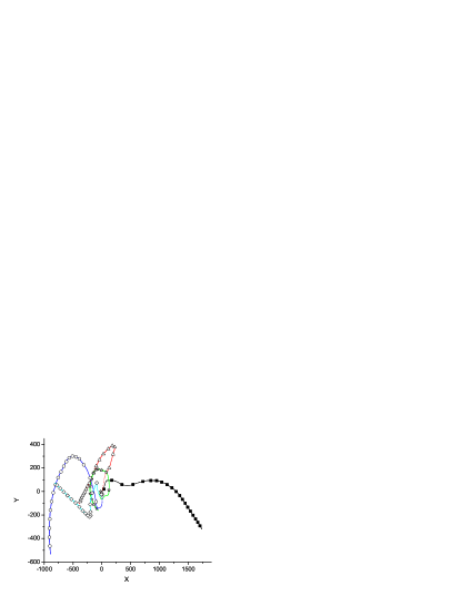
Figure 3: (Color online) Center of mass position of five different clusters growing from $10^{5}$ to $5\cdot 10^{7}$ particles, with the interval of $2\cdot 10^{6}$. See discussion for details.

On average, clusters are quite uniform when looking for the average displacement of CoM. We estimate the average angle $\langle\phi\rangle=-0.01504998(\pm 0.05535)$ of CoM (in the interval $[-\pi;\pi]$) to be close to zero, while the angle variance is approximately $\sqrt{\langle\phi^{2}\rangle-{\langle\phi\rangle^{2}}}=1.76$. This is very close to the value one can find assuming that $\phi$ is uniformly distributed in given interval: $\langle\phi\rangle=0$ and $\sqrt{\langle\phi^{2}\rangle-{\langle\phi\rangle^{2}}}=\pi/\sqrt{3}\approx 1.81$.

There have been several attempts in the literature to relate the CoM distance from the origin $R_{M}$ to the expression (2), defined as

$$R_{M}(n)=\sqrt{\frac{1}{K}\sum_{k=1}^{K}\left(\frac{1}{N}\sum_{i=1}^{N}(\vec{r_{i}})\right)^{2}},$$

where $K$ is the number of clusters. We, however, find no reason for such a connection, because $(X,Y)$ changes rather randomly. One can think of it as of a random walk in the plane, reflecting the competition between the growing activity of the branches. One thus expects the corresponding exponent to be equal to $d=2$ (and not to $D\approx 1.71$) in the limit of the infinite cluster size. Yet, the rare events such as the active branch growth effectively lower this value. We have found, that at large cluster sizes the generated exponent may be estimated as $1.8558(13)$ which is notably larger that $D\approx 1.71$. The dependence of $R_{M}(N)$ is plotted in Figure 4 with solid black line, the dash line is the fit, and dots line corresponds to the slope equal to 1/2 (reverse exponent).

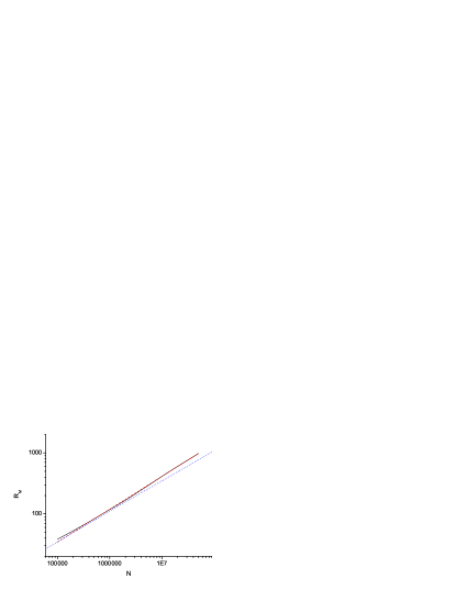
Figure 4: (Color online) Dependence of center of mass position $R_{M}(N)$ with the cluster size $N$, as calculated averaging over 1000 cluster with $5\cdot 10^{7}$ particles. Dashed line is a fit to $R_{M}(N)$ and dotted line have a slope 1/2.

One can calculate the radius of the cluster by either (i) choosing the origin (0,0) as a reference point, or (ii) by choosing a temporary CoM position in the $(X,Y)$ plane as a reference point in the estimation of radii given in Table 1. It turns out that the fractal dimension calculated by means of either of the recipes is the same within the computational error as one can see comparing the second and third columns in the table 2. However, this effect shows the additional possible reason for high fluctuation rates in DLA cased by the unique random branch structure of each cluster.

	$r$ to seed	$r$ to center-of-mass
$R_{\rm dep}$	1.71111(59)	1.71112(60)
$R_{2}$	1.71155(29)	1.71149(54)
$R_{g}$	1.71149(30)	1.71133(30)

Table 2: Fractal dimension estimated by the standard method using the stick distance $r$ to the seed (second column) and to the center-of-mass (third column) as estimated for the number of typical lengthes.

V Fractal dimension estimation: variable probe particles

A common technique of enhancing the precision of computations is the noise reduction in DLA. In doing so, one selects only the most probable events by attaching the hit counters to each particle of the cluster. The new particle is added to the particular old particle when the old particle is hit with some prescribed number of times. Similarly, the same procedure can be used when calculating the harmonic measure averages. Tips are the most probable places to grow, and at the same time the fluctuations at the tips are more strongly associated with the drastic changes in the cluster geometry, which is reflected in the competing growing of the branches, in the birth of the new branches, and in the mutual screening of branches. The internal (frozen) part of the cluster surface, which is screened in the fjords and carry the small part of the measure, may give some contribution to the harmonic averages due to its length which can be large. So, we suppose that the internal part of the DLA cluster may contribute to the average. To check on this point, we introduce the variable size of the probe particles. We choose the size of the particles which we used to build the cluster to be the unit of the length, and measure in this units the probe particles size, $\delta$. Larger particles increase the growth probabilities at the tips, while smaller particles will penetrate dipper in the fjords, and redistribute harmonic measure shifting the part of the growth weight from the tips to the fjords (see next Section for details).

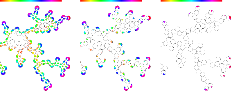
Figure 5: (Color online) Fragment of the cluster with $N=10^{3}$ particles. Intensity of the segments is proportional to the logarithm of the hit probabilities, corresponding to the probe particles of size $\delta=0.1,1$, and $10$, from left to right. Probabilities are larger near the tips and smaller inside the fjords. For lower $\delta$ the bigger part of the cluster surface is touched by probe particles.

Figure 5 illustrates the variation of the harmonic measure estimation with the probe particle size $\delta$. Here the intensity reflects the probability (in the log scale) for the particle to hit the given segment of the cluster. The probe particles of the size $\delta=10$ hit only few particles at the tips and never go inside the fjords. Only this hottest part of the cluster contributes to the harmonic measure estimation. The particles of the size $\delta=1$ touch the bigger part of the surface but still there are regions inaccessible to them. The smaller particles of the size $\delta=0.1$ (recall that this size is less than that of the building particles of the size 1) touch visibly the larger part of the cluster surface, penetrating deeper into the fjords.

Two features contribute to the fjord screening: the size of a probe particle and the bottleneck configuration. Even if a particle fits into the bottleneck, the probability for it to pass is very small if the size of the particle is comparable to the bottleneck width. In other words, the effective channel width is somewhat narrower than the bottleneck width. Using the variable size probe particles we suppress the influence of the bottleneck and can thus measure the lower probabilities at the fjord surface. At the first glance, our approach looks opposite to the noise reduction method, which cuts the parts of the surface with the low harmonic measure. In fact, this contrast is misleading, because noise reduction method affects the growth process of the cluster, and our method affects the measurement process of the harmonic measure, and leads to the higher precision of the estimation of harmonic averages.

One can think of our approach as of the canonic measurement of the length of the coast: the smaller the ruler, the bigger the coast length is Mandelbook . In our case, the smaller probe particles, the longer the reachable surface is, with the cut-off on the scale of the bulk particles.

V.1 Number of particles on the surface

By varying the size of probe particles we change the reachable effective cluster surface. The number of particles on the surface reachable during the probing process is shown in Figure 6. Solid line on the picture is the fit to the expression

$$N_{reach}=N_{surf}/(1+\delta/\delta_{0})^{\alpha}$$ (3)

with $\alpha=0.91(1)$, $\delta_{0}=2.23(6)$ and $N_{surf}=45697(187)$. $N_{surf}$ is a total number of surface particles in cluster, those reachable by probe particles with infinitesimal size, and clusters size fixed to $10^{6}$. Thus, in the measurements with $10^{6}$ probe particles one can touch only about $N_{surf}\approx 45700$. The number of reachable particles for $\delta=1$ is lower by the factor of $1.4$ than for particles of size $\delta=0.1$. The number of reachable particles is the complex function of the probe particle size and of the number of probe particles. The best way to fill the whole surface of the cluster with probes is to find the limit $N_{probes}\rightarrow\infty$. But this is very time consuming procedure.

Figure 6: Number of particles on the surface reachable by probe particles of size $\delta$. Measured by $10^{6}$ probe particles and clusters of size $10^{6}$.

V.2 $D$ in the limit of vanishing probe particle size

The fractal dimension of the aggregate turns out to depend also on $\delta$, and the effective fractal dimension is now a function of two variables, $D(N,\delta)$. We are interested in the double limit $D=\lim_{N\rightarrow\infty,\delta\rightarrow 0}D(N,\delta)$. Let us first find the limit of the vanishing $\delta$, which gives us the $D(N)$ dependence:

$$D(N)=\lim_{\delta\rightarrow 0}D(N,\delta)$$ (4)

with the help of the fit

$$D(\delta,N)=D(N)+A\delta^{\beta}.$$ (5)

Figure 7: Fractal dimension $D(\delta,N)$ as a function of the probe particle size $\delta$ for different cluster size. Inset: $D(\delta,N)$ is shown as a function of $N$ for the set of $\delta$ values. Lines are the guide for the eye. See text for details.

We calculated harmonic measure averages with the set of probe particles sizes: $\delta=0.1,$ 0.3, 1, 3, 10, 30, and 100. The resulting fractal dimension $D(\delta,N)$ is shown in Figure 7 as function of $\delta$ for $N=5$, 10, 15, …, 50 millions of particles. Fractal dimension $D(\delta,N)$ as a function of N for the set of $\delta$ is shown in the inset of Figure 7, the topmost curve corresponds to $\delta=100$, while the lowermost - to $\delta=0.1$.

Result of the data fit to Expr. (5) are shown in Figure 8.

Surprisingly, in the limit of the vanishing size of probe particles fractal dimension become monotone function. As $N$ goes to infinity $D(N)$ reaches its asymptotic value with approximate behavior (fit using the last 6 data points) $D(N)=D+4.2\cdot 10^{12}/N^{2.17}$ which gives the high precision of fractal dimension estimation $D=1.7100(2)$.

V.3 Errors estimation

Making use of the least square fitting $\log(R_{\rm dep}^{hm})$ to $\log N$ when calculating the fractal dimension of a single cluster $D_{k}(N,\delta)$, one can estimate an error on its determining. As has been mentioned above, the clusters are unique, and this results in large fluctuations of the fractal dimension over ensemble. This means that the error in the $D(N,\delta)$ averaged over the ensemble depends mostly on its variation, while the errors in each $D_{k}(N,\delta)$ are several times smaller. The next stage of out calculation is constructing the nonlinear square fitting (NLSF) to the equation (5) where all the data points have a weight, iversely proportional to the error, assosiated with the point (instrumental error in terms of Origin program). Resulting $D(N)$ curve is then fitted by the expression $D(N)=D+A/N^{B}$ and the error for $D$ is again estimated with the help of NLSF.

Figure 8: Fractal dimension as function of $N$ for the limiting value of $\delta=0$. It reach value $D=1.7100(2)$ (plotted with the dotted line) in the limit of large cluster size $N$.

VI Probability distribution function

Harmonic-measure averages can be written in a form $R_{\rm dep}=\int P(r,N)rdr$, where $P(r,N)$ is the probability for a particle to stick to the cluster with $N$ particles at the distance $r$ from the origin (or from center-of-mass as discussed in Section IV). This probability acquires a Gaussian form ms-PZ ; nms-SBBS ; Lee upon averaging over the ensemble of clusters. It is not so if one calculates $P(r,N)$ at the surface of a single cluster realization; rare events associated with the particular shape contribute essentially to the probability function. It was proposed in DLA-MS that fluctuations in $P(r,N)$ are responsible for multiscaling issue.

We measure $P(r,N,\delta)$ for a fixed cluster size $N=2\cdot 10^{7}$ and the size of the probe particles $\delta$, and average over the ensemble of 1000 clusters. The resulting function $\overline{P(r,N)}$ is shown in Figure 9. On the scale of the figure, all lines practically coincide. Fluctuations of the measured probability around the Gaussian form are visible despite the large number of clusters we use for averaging.

The effect of the variation in the probe particle size on the probability function may be investigated with the use of the difference,

$$\delta P(r,N)=P(r,N,\delta)-P(r,N,\delta\rightarrow 0),$$ (6)

which we approximate with the difference taken for the smallest used probe particle size $\delta=0.1$, $\delta P(r,N)=P(r,N,\delta)-P(r,N,\delta=0.1)$.

The variation $\delta P(r,N)$ demonstrates the sin-like shape, with zero variation for any $\delta$ at the distance corresponding to the average deposition radius $R_{\rm dep}$. The finiteness of the probe particles leads to the increase of the probability for $r>R_{\rm dep}$ and probability decreases at distances $r<R_{\rm dep}$ (shown with arrow in Figures 9 and 10. The amplitude of $\delta P(r,N)$ varies with $\delta$ as $\delta^{0.78(1)}$. So we can normalize functions $\delta P(r,N;\delta)$ with the multiplier $\delta^{-0.78}$, $G(r,N,\delta)=\delta P(r,N,\delta)\delta^{-0.78}$. The set of this functions is presented in Figure 10. All of them completely coincide well. The only exception is for $\delta=0.3$ but this is clearly due to approximation $P(r,N,\delta\rightarrow 0)\approx P(r,N,\delta=0.1)$ used in expr (6). It seems, therefore, that finite size of the probe particles will case the systematic overestimation of the fractal dimension.

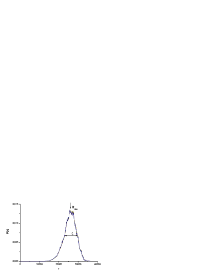
Figure 9: Probability to stick at distance $r$ for different $\delta$ averaged over 1000 clusters with size $N=2\cdot 10^{7}$.

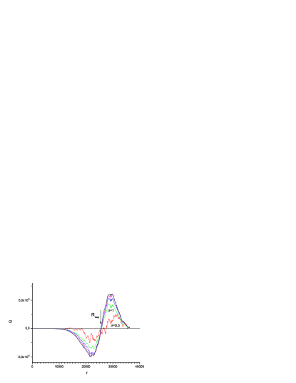
Figure 10: (Color online). Normalized change of probability to stick at distance $r$ for different $\delta$ relative $\delta=0.1$. Fixed point is at $R_{\rm dep}$. Clusters size $N=2\cdot 10^{7}$.

VII Discussion

Utilizing the variable probe particles for the harmonic measure estimations allows analysis of fractal dimension as a function of two variables. Fixing cluster size and taking the limit of the vanishing size of a probe particle effectively smoothes out the effects of the sample fluctuations as is seen from the monotonic variation of the fractal dimension with the growing cluster size. This contrasts favorably the conventional methods where the fractal dimension can oscillate with the cluster size making the convergence of the results very slow. As a result using variable size particles, one can extract the value of the fractal dimension from $D(\delta,N)$ with the unprecedented high precision: we have found that $D=1.7100(2)$ for the off-lattice DLA cluster in the plane.

We like to stress the accuracy of the above estimations as compared to those obtained by the traditional methods mentioned in Tables 1 and 2. Technically, all the estimations are compatible within the $2\sigma$ accuracy and, as it seems, may be treated with the equal confidence. The major difference of the values estimated with the help of varying probe size, is that it is estimated not as a single random variable but as the asymptotic value of some regular function as shown in Figure 8. Our approach corresponds to the variation of the ruler scale in the conventional estimation of the fractal dimension Mandelbook .

The major result of our work is that for the first time we have reached a quality of the data which can offer reliable quantitative answers. In particular, the obtained value of fractal dimension allows to rule out the d=17/10 hypothesis proposed by Hastings about 10 years ago Hastings97 . Furthermore, our technique can be used for the analysis of fractal dimension as a function of the lattice symmetry (d=3,4,5,6,7,8 and off-lattice corresponds to infinity). The next interesting question to address is the distribution of the harmonic measure near the tips and inside the fjords, where one can expect our approach to be most effective.

VIII Acknowledgements

This work was supported by the U.S. Department of Energy Office of Science through contract No. DE-AC02-06CH11357 and the Program. A.Yu.M. thanks Prof. G. Eilenberger and Landau Scholarship Committee for support and Prof. H. Müller-Krumbhaar and Prof. E. Brener for the kind hospitality and useful discussions.

References

- (1) A. Bunde and S. Havlin, eds., Fractals and Disordered Systems (Springer, Berlin, 1996).
- (2) T. C. Halsey, Physics Today 53 (2000) 36.
- (3) T.A. Witten and L.M. Sander, Phys. Rev. Lett. 47 (1981) 1400.
- (4) L. Niemeyer, L. Pietronero, H.J. Wiesmann, Phys. Rev. Lett., 52 (1984) 1033.
- (5) P.G. Saffman and G.I. Taylor, Proc. R. Soc. London A 245, 312 (1958).
- (6) F. Barra, B. Davidovitch, A. Levermann, and I. Procaccia, Phys. Rev. Lett. 87 134501 (2001).
- (7) H.G.E. Hentschel, A. Levermann, and I. Procaccia Phys. Rev. E 66, 016308 (2002).
- (8) M.B. Hastings and L.S. Levitov, Physica D 116 (1998) 244.
- (9) M.B. Hastings, Phys. Rev. Lett. 88 (2002) 055506.
- (10) O. Schramm, Israel J. Math. 118 (2000) 221; G.F Lawler, P. Schramm, and W. Werner, Acta Math. 187(2) (2001) 237; ibid. 187(2) (2001) 275.
- (11) J. Cardy, Annals Phys. 318 (2005) 81.
- (12) T.A. Rostunov and L.N. Shchur, JETP 95, 145 (2002).
- (13) A. Yu. Menshutin and L.N. Shchur, Phys. Rev. E 73 (2006) 011407.
- (14) A. Yu. Menshutin, L.N. Shchur, V.M. Vinokur, Phys. Rev. E 75 (2007) 010401(R).
- (15) R.C. Ball and R.M. Brady, J. Phys. A 18 (1985) L809.
- (16) S. Tolman and P. Meakin, Physica A 158 (1989) 801; Phys. Rev. A 40 (1989) 428.
- (17) P. Meakin, R.C. Ball, P. Ramanlal, L.M. Sander 35 (1987) 5233.
- (18) E. Sander, L. M. Sander, R. M. Ziff, Computers in Physics 8 (1994), 420-425; L.M. Sander, Contemporary Physics 41 (2000), 203-218.
- (19) H. Kaufman, A. Vespignani, B.B. Mandelbrot, and L. Woog, Phys. Rev. E 52 (1995) 5602.
- (20) S. Redner, Guide to First-Passage Processes (Cambridge University Press, New York, 2001).
- (21) B.B. Mandelbrot, The fractal geometry of nature (W.H. Freeman and Company, New York, 1982)
- (22) M. Plischke and Z. Rácz, Phys. Rev. Lett. 53 (1984) 415.
- (23) E. Somfai, R.C. Ball, N.E. Bowler, L.M. Sander, Physica A 325 (2003) 19.
- (24) J. Lee, S. Schwarzer, A. Coniglio, H.E. Stanley, Phys. Rev. E 48 (1993) 1305.
- (25) M.B. Hastings, Phys. Rev. E 55 (1997) 135.