The thermodynamics and roughening of solid-solid interfaces

Abstract

The dynamics of sharp interfaces separating two non-hydrostatically stressed solids is analyzed using the idea that the rate of mass transport across the interface is proportional to the thermodynamic potential difference across the interface. The solids are allowed to exchange mass by transforming one solid into the other, thermodynamic relations for the transformation of a mass element are derived and a linear stability analysis of the interface is carried out. The stability is shown to depend on the order of the phase transition occurring at the interface. Numerical simulations are performed in the non-linear regime to investigate the evolution and roughening of the interface. It is shown that even small contrasts in the referential densities of the solids may lead to the formation of finger like structures aligned with the principal direction of the far field stress.

I Introduction

The formation of complex patterns in stressed multiphase systems is a well known phenomenon. The important studies of Asaro and Tiller Asaro72 and Grinfeld Grinfeld86 brought attention to the morphological instability of stressed surfaces in contact with their melts or solutions. In the absence of surface tension, small perturbations of the surface increase in amplitude due to material diffusing along the surface from surface valleys, where the stress and chemical potential is high, to surrounding peaks where the stress and chemical potential is low. Important examples of instabilities at fluid-solid interfaces include defect nucleation and island growth in thin films  Srolovitz88 ; Gao99 , solidification Mullins57 and the formation of dendrites and growth of fractal clusters by aggregation Meakin98 . The surface energy increases the chemical potential at regions of high curvature (convex with respect to the solution or melt, at the peaks) and reduces the chemical potential at region of low curvature (at the valleys) and this introduces a characteristic scale below which the interface is stabilized.

In systems where the fluid phase is replaced by another solid phase, i.e. solid-solid systems, the interface constraints alter the local equilibrium conditions. Here we study a general model for a propagating interface between non-hydrostatically stressed solids. The interface propagates by mass transformation from one phase into the other. The phase transformation is assumed to be local, i.e. the distance over which the solid is transported via surface diffusion or solvent mediated diffusion is negligible compared to other relevant scales of the system. Although the derivations apply to a diffuse interface, we shall here treat only coherent interfaces, where there is no nucleation of new phases or formation of gaps between the two solids  Robin74 ; Larche78 , in the sharp interface limit. For example, in rocks such processes appear at the grain scale in ”dry recrystallization” Kamb58 ; Fletcher73 . Common examples of coherent interfaces that migrate under the influence of stress include the surfaces of coherent precipitates (stressed inclusion embedded in a crystal matrix) Robin74 and interfaces associated with isochemical transformations. Most studies of solid-solid phase transformations have been limited to the calculation of chemical potentials in equilibrium and have provided little insight into the kinetics. Here we investigate the out of equilibrium dynamics of mass exchange between two distinct solid phases separated by a sharp interface. We expand on the recent work presented in PRL08 where we studied the phase transformation kinetics controlled by the Helmholtz free energy. It was shown that a morphological instability is triggered by a finite jump in the free energy density across the interface, and in the non-linear regime this leads to the formation of finger like structures aligned with the principal direction of the applied stress.

In the majority of solid-solid phase transformation processes, the propagation of the interface is accompanied by a change in density. For this reason the density is an important order parameter that quantitatively characterizes the difference between the two phases. We consider two types of phase transitions underlying the kinetics, first order and second order, which result in fundamentally different behaviors at the phase boundary. A first order phase transition occurs when the two phases have different referential densities and it typically results in morphological instability along the boundary whereas a second order phase transition may either stabilize or destabilize the interface depending on Poisson’s ratios of the two phases. A simple sketch of the stability diagram is outlined in Fig. 1 for relative values of density and shear modulus of the two phases.

Figure 1: Sketch of a stability diagram for the growth rate of a sharp interface separating two solid materials. The axes show relative values of the shear modulus and density of the phases. As it will be shown in Sec. III, the symmetry of the diagram is broken by the values of the Poisson’s ratios.

The article consists of five sections. In Sec. II we derive a general equation for the kinetics for mass exchange at a solid-solid phase boundary separating two linear elastic solids. We utilize the derived equations on a simple one dimensional example and offer a short discussion of the order of the phase transition underlying the kinetics. We proceed in Sec. III with a linear stability analysis of the full two-dimensional problem. In two dimensions, the phase transformation kinetics gives rise to the development of complex patterns along the phase boundary. While we solve the problem analytically for small perturbations of a flat interface, things become more complicated in the non-linear regime, and we resort to numerical simulations based on the combination of a Galerkin finite element discretization with a level-set method for tracking the phase boundary. In Sec. IV, numerical results are presented together with discussions. Finally in Sec. V we offer concluding remarks.

II General phase transformation kinetics

Although the equations that we derive for the exchange of a mass element between two solid phases in a non-hydrostatically stressed system apply to more general settings, we limit ourselves to the study of two solids separated by a single sharp interface. The solids are stressed by an external uniaxial load as illustrated in Fig. 2. In the referential configuration, a solid phase is assumed to have a homogenous mass density, $\rho^{0}$, defined per unit undeformed volume occupied by that phase. After the deformation, the densities are functions of space $x$ and time $t$, i.e. $\rho_{1}(x,t)$ and $\rho_{2}(x,t)$. The average density of the two-phase system is denoted by $\rho(x,t)$. Finally, the mass fraction for phase $1$ is denoted by $c$. In this notation, the mass fraction of phase $2$ becomes $1-c$.

For non-vanishing densities, the mass-averaged velocity is defined as

$$\bar{v}=cv_{1}+(1-c)v_{2}.$$ (1)

Throughout the text, the mass average of any quantity is indicated by a bar. Similarly, the average specific free energy density is given by

$$\bar{f}=cf_{1}+(1-c)f_{2}.$$ (2)

The total specific volume is related to the real densities in the deformed state, $\rho_{1}(x,t)$ and $\rho_{2}(x,t)$ by

$$\rho^{-1}=c\rho_{1}^{-1}+(1-c)\rho_{2}^{-1}.$$ (3)

The interface separating the two phases is tracked by the zero level of a scalar field $\phi(x,t)$ passively advected according to the equation

$$\frac{\partial\phi}{\partial t}+W\left|\nabla\phi\right|=0,$$ (4)

where $W$ is the normal velocity of the surface. It follows that the interface is given by the zero level set

$$\Gamma=\left\{x|\phi(x,t)=0\textrm{, for all }t\right\}.$$ (5)

The scalar field is constructed such that phase 1 occupies the domain in which $\phi(x,t)>0$ and phase 2 occupies the domain in which $\phi(x,t)<0$, see Fig. 2. In this notation, the mass fraction may be expressed as the characteristic function of the scalar field,

$$c(x,t)=H\left(\phi(x,t)\right)=\left\{\begin{array}[]{c}1\textrm{, if }\phi(x,t)>0\\ \frac{1}{2}\textrm{, if }\phi(x,t)=0\\ 0\textrm{, otherwise.}\end{array}\right.$$ (9)

In the subsequent analysis, we make use of the following relations (see e.g. Trusk98 )

$$\nabla_{i}c=n_{i}\delta_{\Gamma},\quad\partial_{t}c=-W\delta_{\Gamma},$$ (10)

where $n_{i}={\nabla_{i}\phi}/{|\nabla\phi|}$ is the normal unit vector of the interface, $W=-{\partial_{t}\phi}/{|\nabla\phi|}$ is the normal velocity and $\delta_{\Gamma}=|\nabla\phi|\delta(\phi)$ is the surface delta function.

Taking the gradient of the averaged velocity from Eq. (1) and using the above identities, the following relation is obtained

$$\nabla_{i}\bar{v}_{j} = \frac{\partial\bar{v}_{j}}{\partial c}\nabla_{i}c+c\nabla_{i}v_{1,j}+(1-c)\nabla_{i}v_{2,j}$$ (11)

$$= \frac{\partial\bar{v}_{j}}{\partial c}n_{i}\delta_{\Gamma}+\overline{\nabla_{i}v_{j}}.$$

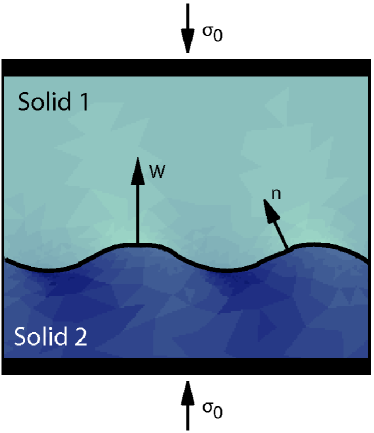
Figure 2: (color online) Two solids separated by a sharp interface. A compressional force is applied at the margins in the vertical direction

II.1 Kinetics of the phase transformation

The system must satisfy fundamental conservation principles for the mass, momentum, energy and entropy. Let us denote the material time derivative with respect to the mass-averaged velocity by a dot, i.e. $\dot{\Theta}=\partial_{t}\Theta+\bar{v}_{i}\nabla_{i}\Theta$. Then, the local mass conservation can be written in the form

$$\dot{\rho}=-\rho\nabla_{i}\bar{v}_{i}.$$ (12)

and the local momentum balance can be written in the form

$$\rho\dot{\overline{v}_{i}}=\nabla_{j}\sigma_{ij},$$ (13)

where $\sigma_{ij}$ is the stress tensor.

The mass fraction of phase 1 satisfies the advection-reaction equation given by

$$\rho\dot{c}=Q\delta_{\Gamma},$$ (14)

where the mass exchange rate $Q$ is confined to the interface by the delta-function (in the sharp interface limit). Mass transport by diffusion is negligible in the reaction dominated regime. This is a valid approximation when the characteristic length $\ell=\cal{D}/W$, where $\cal D$ is the diffusion coefficient and $W$ is the velocity of the interface, is small compared with other relevant microscopic length scales. That is material diffusion occurs on a time scale much longer than any other relevant time scale in the system or equivalently the characteristic length scale formed from the diffusion constant and solidification or precipitation rate is small compared to other relevant microscopic scales.

In the linear kinetics, the mass exchange rate is now derived from the requirement that the entropy production has a positive quadratic form. We start by expressing the conservation of specific energy density $e$ in the form

$$\rho\dot{\bar{e}}=\sigma_{ij}\nabla_{i}\bar{v}_{j},$$ (15)

where $\bar{v}^{2}=cv_{1}^{2}+(1-c)v_{2}^{2}$ since the cross term vanishes in the limit of a sharp interface.

At equilibrium

$$\bar{e}=\bar{f}+T\bar{s},$$ (16)

where the free energy is assumed to be a function of the local strain and the composition, i.e. $\bar{f}=\bar{f}(\bar{\epsilon}_{ij},c)$. By inserting the energy conservation equation, Eq. (15), into the time derivative of this equation, under constant temperature conditions, the expression

$$\rho T\dot{\bar{s}}=\sigma_{ij}\nabla_{i}\bar{v}_{j}-\rho\frac{\partial\bar{f}}{\partial\bar{\epsilon}_{ij}}\dot{\overline{\epsilon_{ij}}}-\rho\frac{\partial\bar{f}}{\partial c}\dot{c},$$ (17)

is obtained. The phase transformation is assumed to be slow and isothermal. From Eqs. (2) and (11) it follows that

$$\rho T\dot{\bar{s}}=\sigma_{nj}\frac{\partial\bar{v}_{j}}{\partial c}\delta_{\Gamma}+\sigma_{ij}\overline{\nabla_{i}v_{j}}-\rho\frac{\partial\bar{f}}{\partial\bar{\epsilon}_{ij}}\dot{\overline{\epsilon_{ij}}}-\frac{\partial f}{\partial c}\rho\dot{c}.$$ (18)

Given that the strain rate is $\dot{\epsilon}_{ij}=1/2(\nabla_{i}v_{j}+\nabla_{j}v_{i})$ and using the symmetry of the stress tensor, we arrive at the expression

$$\rho T\dot{\bar{s}}=\sigma_{nj}\frac{\partial\bar{v}_{j}}{\partial c}\delta_{\Gamma}+\left(\sigma_{ij}-\rho\frac{\partial\bar{f}}{\partial\bar{\epsilon}_{ij}}\right)\dot{\overline{\epsilon_{ij}}}-\frac{\partial f}{\partial c}Q\delta_{\Gamma},$$ (19)

where $\sigma_{nj}=\sigma_{ij}n_{i}$ is the stress vector at the interface. From Eqs. (11) and (12) and using an equation of state of the form $\rho(\bar{\epsilon}_{ij},c)=\rho^{0}(c)(1-\bar{\epsilon}_{ii})$ it follows that,

$$\frac{\partial\rho}{\partial c}\dot{c}+\frac{\partial\rho}{\partial\bar{\epsilon}_{ij}}\dot{\overline{\epsilon_{ij}}} = -\frac{\partial v_{n}}{\partial c}\rho\delta_{\Gamma}-\rho\overline{\nabla_{i}v_{i}}\Rightarrow$$

$$\frac{1}{\rho}\frac{\partial\rho}{\partial c}Q\delta_{\Gamma}-\rho^{0}\dot{\overline{\epsilon_{ii}}} = -\frac{\partial v_{n}}{\partial c}\rho\delta_{\Gamma}-\rho\overline{\nabla_{i}v_{i}}\Rightarrow$$

$$\frac{\partial}{\partial c}\left(\frac{1}{\rho}\right)Q=\frac{\partial v_{n}}{\partial c} ,\quad \rho^{0}\dot{\overline{\epsilon_{ii}}}\approx\rho\overline{\nabla_{i}v_{i}}.$$

Using Eq. (3) for the density, the jump in the material velocity is related to the reaction rate by

$$\frac{\partial v_{n}}{\partial c}=Q\frac{\partial}{\partial c}\left(\frac{1}{\rho}\right).$$ (20)

The direction of the kinetics is constrained by the second law of thermodynamics which can be expressed in the continuum form as

$$\rho\dot{\bar{s}}+\nabla_{i}J^{s}_{i}=\Pi_{s},$$ (21)

where $J^{s}_{i}$ is the entropy flux density and $\Pi_{s}\geq 0$ is the entropy production rate. We consider the case where the entropy flux is negligible (in the absence of mass and heat fluxes) and therefore set $J_{s}=0$. Combining Eqs. (19) and (21), it can be seen that the positive entropy production rate leads to the condition

$$\left(\sigma_{nn}\frac{\partial}{\partial c}\left(\frac{1}{\rho}\right)-\frac{\partial\bar{f}}{\partial c}\right)Q\delta_{\Gamma}+\left(\sigma_{ij}-\rho\frac{\partial\bar{f}}{\partial\bar{\epsilon}_{ij}}\right)\dot{\overline{\epsilon_{ij}}}=T\Pi_{s}\geq 0$$ (22)

on the reaction rate. We now define a constitutive relation that couples the stress to the strain via the Helmholtz free energy,

$$\sigma_{ij}=\rho\frac{\partial\bar{f}}{\partial\bar{\epsilon}_{ij}}.$$ (23)

From Eq. (22) we observe that the entropy is produced only at the interface, and in the linear kinetics regime the reaction rate is proportional to (see e.g. entprod ),

$$Q\approx K\left(\sigma_{nn}\frac{\partial}{\partial c}\left(\frac{1}{\rho}\right)-\frac{\partial\bar{f}}{\partial c}\right),$$ (24)

where $K>0$ is a system specific constant.

The normal velocity of a sharp interface is obtained by integrating Eq. (14) across the interface and taking the singular part of it,

$$W\approx\bar{v}_{n}-\frac{K}{\rho}\left\llbracket\sigma_{nn}\frac{1}{\rho}-f\right\rrbracket.$$ (25)

Here we introduce the jump in the quantity $a$ from one phase to another $\left\llbracket a\right\rrbracket:=a_{1}-a_{2}$, where $a_{i}$ is the value of $a_{i}$ in phase $i$ outside the interface zone as the interface is approached. The additional interfacial jump conditions of the total mass and force balance from Eqs. (12) and (13) are given by

$$\llbracket\rho(W-v_{n})\rrbracket=0$$ (26)

$$\llbracket\sigma_{ij}n_{j}\rrbracket=0.$$ (27)

In general, surface energy $\gamma$ and surface stresses may have an important effect on the kinetics at the phase boundary with high curvature $\mathcal{K}$, therefore the expressions given above are modified to take this into account. For this purpose we utilize the Cahn-Hilliard formalism Cahn58 of a diffuse interface. The surface energy is obtained by allowing the Helmholtz free energy density to be a function of the mass fraction gradients, i.e.

$$\rho\bar{f}(\bar{\epsilon}_{ij},c,\nabla c)=\rho\bar{f}_{0}(\bar{\epsilon},c)+\frac{\kappa_{1}}{2}|\nabla c|^{2},$$ (28)

where $\kappa_{1}$ is a small parameter related to the infinitesimal thickness of the interface and $\bar{f}_{0}$ is the homogenous free energy density introduced above. Because the composition gradient is small everywhere except for a thin zone at the interface, the free energy can be separated into bulk and surface contributions. If we now take the limit of vanishing surface thickness and follow the derivations in the appendix we obtain the general jump condition for the normal force vector,

$$\llbracket\sigma_{nn}\rrbracket=-2\mathcal{K}\gamma.$$ (29)

In the aforementioned expression of the interfacial velocity Eq. (25) the normal stress vector was continuous across the interface. In the presence of surface tension, the normal velocity is altered by an additional contribution from the surface energy,

$$W\approx v_{1,n}+\frac{K}{\rho_{1}}\left(\left\llbracket f\right\rrbracket-\langle\sigma_{nn}\rangle\left\llbracket\rho^{-1}\right\rrbracket+2\mathcal{K}\gamma\langle\rho^{-1}\rangle\right),$$ (30)

where we have used the interface average defined as $\langle a\rangle=1/2(a_{1}+a_{2})$.

II.2 Example: Phase transformation kinetics in a one dimensional system

Figure 3: One dimensional system undergoing phase transformation

We start out considering the phase transformation kinetics of a one dimensional system composed of two linear elastic solids separated by a single interface. A force $\sigma$ is applied at the boundary of the system (see Fig. 3) and each solid phase is represented by its Young’s modulus $E_{i}$ ($i=1,2$), undeformed density $\rho_{i}^{0}$ and length $L_{i}^{0}$. In the deformed state when the external force is applied the length becomes $L_{i}=L_{i}^{0}\left(1+\sigma/{E_{i}}\right)$ and the density $\rho_{i}=\rho_{i}^{0}L_{i}^{0}/L_{i}$. The specific free energy is given by

$$f=\frac{\sigma^{2}}{2}\left(\frac{c}{\rho_{1}(E_{1}+\sigma)}+\frac{1-c}{\rho_{2}(E_{2}+\sigma)}\right).$$ (31)

In the following, we do not allow new phases to nucleate within the solids and limit our considerations to the propagation of a single interface separating the solids. The system is assumed to be isothermal and no diffusion of mass takes place. The interface moves as one phase, slowly transforms into the other and an amount $\rho_{1}dL_{1}$, of solid 1 is replaced by an amount $\rho_{2}dL_{2}$ of solid 2, with conservation of the total mass. The phase transformation is assumed to be irreversible and to occur on time scales that are much larger than the time it takes for the system to relax mechanically under the deformational stresses.

In the one dimensional setting the local mass exchange rate is given by a linear kinetic equation, Eq. (24), of the form

$$\dot{m}_{1}=-K\left\llbracket\frac{\sigma^{2}}{2\rho^{0}E}-\frac{\sigma}{\rho}\right\rrbracket=K\left\llbracket\frac{\sigma^{2}}{2\rho^{0}E}+\frac{\sigma}{\rho^{0}}\right\rrbracket,$$ (32)

with $K>0$. In most cases, the contribution from the jump in the elastic energy density will be small compared to the contribution from the work term (because $\sigma/E\ll 1$, within the linear elasticity regime). The change in the total length will in general follow the sign of the stress

$$\dot{L} = \dot{L}_{1}(1-\frac{\rho_{1}}{\rho_{2}})=\dot{m}_{1}\left\llbracket\frac{1}{\rho}\right\rrbracket$$

$$= K\left\llbracket\frac{\sigma^{2}}{2E\rho^{0}}+\frac{\sigma}{\rho^{0}}\right\rrbracket\left\llbracket\frac{1}{\rho^{0}}+\frac{\sigma}{E\rho^{0}}\right\rrbracket.$$

If the densities in the undeformed states are identical, $\rho_{1}^{0}=\rho_{2}^{0}$, the change in the total length is given by

$$\dot{L}=K\frac{\sigma^{3}}{2\rho^{0}}\left\llbracket\frac{1}{E}\right\rrbracket^{2},$$ (33)

whereas a jump in the referential densities ($\rho^{0}_{1}\neq\rho^{0}_{2}$) will result in a work term given by

$$\dot{L}\approx K\sigma\left\llbracket\frac{1}{\rho^{0}}\right\rrbracket^{2}.$$ (34)

Under a compressional load, the dense phase grows at the expense of the less dense phase (if the two phases have the same Young’s modulus) and the soft phase grows at the expense of the hard phase (if the two phases have the same density), such that overall the system responds to the external force by shrinking. The one-dimensional model cannot predict the morphological stability of the propagating phase boundary in two dimensions. It turns out that the work term destabilizes the propagating boundary under a compressional load.

II.3 First and second order phase transitions: Equilibrium phase diagrams

In the above derivations, the reaction rate is determined by the jump in the Gibbs potential across the phase boundary. Whenever the system is stressed, only one of the two phases will be stable, i.e. the general two phase system will always evolve to an equilibrium state consisting of a single phase. In the absence of an external stress, it is possible for two phases to coexist without any phase transformation taking place. In the one dimensional example, the relevant field variable is the stress $\sigma$ applied to the system and the Gibbs potential is given by (follows from Eq. (32))

$$g(\sigma)=\frac{\sigma^{2}}{2\rho^{0}E}-\frac{\sigma}{\rho}.$$ (35)

In Fig. 4 we show an equilibrium phase diagram in the conjugate pair of variables $\sigma$ and $1/\rho$. If the derivative of the Gibbs potential with respect to the external field $\sigma$ is evaluated at the critical point $\sigma=0$, it can be seen that there are two possible scenarios. The first scenario is a first order phase transition, which occurs whenever there is a jump in the referential densities, i.e. the derivative of the Gibbs potential is discontinuous and the second derivative diverges at the critical point. The other scenario is a second order phase transition, which occurs when the referential densities of the two phases are identical. We then have a jump in the second order derivative whenever Young’s modules of the two phases are dissimilar.

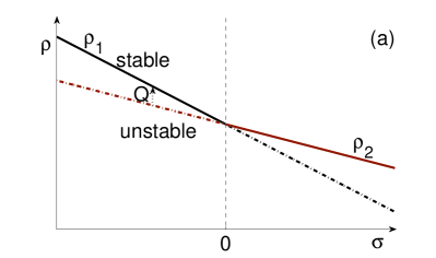
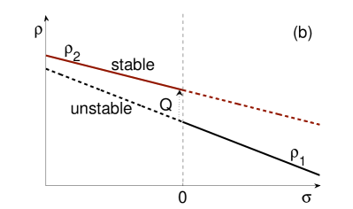
Figure 4: (color online) Part (a) illustrates the phase diagram for a second order phase transition in the $\rho-\sigma$ plane. The solid-solid kinetics will always be directed from the unstable phase (dashed line) to the stable phase as illustrated by reaction path $Q$ marked by the dashed arrow. The slopes of the densities with respect to stress are Young’s modules of the materials. Part (b) illustrates the equilibrium curves of the first order phase transition. For the first order phase transition one would in general expect to see hysteresis effects extending the continuous lines (stable regions) beyond the point $\sigma=0$. Here we have shown an idealized case where such effects are disregarded.

The order of the phase transition has a fundamental impact on the dynamics. In two dimensions a first order phase transition kinetics will generally lead to morphological instabilities of the propagating phase boundary while a second order phase transition will either flatten or roughen the boundary depending on Poisson’s ratios of the two materials. In the next section we analyze the different phase transitions by performing a linear stability analysis.

III Linear perturbation analysis

We now solve the elasto-static Eqs. (13) and (29) together with the kinetics Eqs. (25) and (30) in two dimensions for an arbitrary perturbation to an initially flat interface using the quasi-static version of momentum balance in Eq. (13). In addition to the translational dynamics observed in the one-dimensional system presented above, it turns out, that in two dimensions the interface dynamics is non-trivial and may lead to the formation of finger-like structures. The general setup is shown in Fig. 2 where phase $i$, $i=1,2$, has material parameters $\mu_{i},\nu_{i}$ and $\rho_{i}$, with $\mu_{i}$ being the shear modulus and $\nu_{i}$ being the Poisson’s ratio. In general, the interface velocity depends on its morphology, the 6 material parameters and the external loading $\sigma_{\infty}$. One degree of freedom is removed by rescaling the shear modulus of one phase with the external load.

III.1 Stress field around a perturbed flat interface

In order to evaluate the jump in Gibbs energy density, i.e. $\left\llbracket\mathcal{F}/\rho^{0}+\mathcal{W}\right\rrbracket$, we need to determine the stress field around the interface by solving the elastostatic equations. We have that under plane stress conditions, the local strain energy density can be written on the form

$$\mathcal{F}=\frac{1}{4\mu}\biggl{(}\sigma_{xx}^{2}+\sigma_{yy}^{2}-\frac{\nu}{1+\nu}(\sigma_{xx}+\sigma_{yy})^{2}+2\sigma_{xy}^{2}\biggr{)}$$ (36)

and the work term is defined as

$$\mathcal{W}=-\sigma_{nn}\rho_{i}^{-1}=-\sigma_{nn}\rho_{i,0}^{-1}(1+\mathrm{Tr}(\mathbf{\epsilon})).$$ (37)

The trace of strain is given in terms of stress by

$$\mathrm{Tr}({\bf\epsilon})=\frac{1-2\nu}{2\mu(1+\nu)}(\sigma_{xx}+\sigma_{yy}).$$ (38)

Note that we could as well have formulated the problem under plane strain conditions; however, the generic behavior in both plane stress and strain is the same although the detailed dependence on the material parameters is altered.

We solve the mechanical problem by finding the Airy stress function, $U(x,y)$ Musk53 , which satisfies the biharmonic equation $\Delta^{2}U=0$. Once the stress function has been found, the stress tensor components readily follow from the relations

$$\sigma_{xx}=\frac{\partial^{2}U}{\partial y^{2}},\quad\sigma_{yy}=\frac{\partial^{2}U}{\partial x^{2}},\quad\sigma_{xy}=-\frac{\partial U}{\partial x\partial y}.$$ (39)

The biharmonic equation is solved under the boundary conditions of a normal load applied in the y direction at infinity, i.e. $\sigma_{yy}\rightarrow-|\sigma_{\infty}|<0$ and $\sigma_{xy}=0$ for $y\rightarrow\pm\infty$. The continuity of the stress vector across the interface follows from force balance. In addition we require that $u_{x}(\pm\infty,y)=0$.

For a flat interface, the stress field is homogenous in space. This implies that the Airy stress function is quadratic in $x$ and $y$, with coefficients determined by the boundary conditions. With the boundary conditions specified above, the stress function for the i-th phase can be written in the form

$$U_{i}(x,y)=\frac{|\sigma_{\infty}|}{2}(x^{2}+\nu_{i}y^{2}).$$ (40)

From this stress function we can calculate the Gibbs potential which in the case of dissimilar phases is discontinuous across the interface. The velocity of the phase transformation readily follows from the potential

$$W_{0} \propto \left\llbracket\mathcal{F}_{0}/\rho^{0}+\mathcal{W}_{0}\right\rrbracket=|\sigma_{\infty}|\left(\frac{1}{\rho^{0}_{1}}-\frac{1}{\rho^{0}_{2}}\right)$$ (41)

$$- \frac{|\sigma_{\infty}|^{2}}{4}\left(\frac{1-3\nu_{1}}{\rho^{0}_{1}\mu_{1}}-\frac{1-3\nu_{2}}{\rho^{0}_{2}\mu_{2}}\right).$$

The subscript of the free energy density and the work term refers to an unperturbed interface. From the above equation, we see that when the lower phase is much denser than the upper phase, i.e. $\rho^{0}_{1}\ll\rho^{0}_{2}$, the interface propagates uniformly into the upper phase with a velocity $W\approx|\sigma_{\infty}|\left\llbracket 1/\rho\right\rrbracket>0$, i.e. the denser phase grows into the softer. When the densities are identical or almost identical, $\rho_{2}/\rho_{1}\approx 1$ and the shear modules significantly different, i.e. $\mu_{1}\ll\mu_{2}$. When the two solids phases have identical Poisson’s ratios, $\nu$, we see that the softer phase can only grow into the harder one when $\nu<1/3$.

In the case of an arbitrarily shaped interface separating the two phases, the analytical solution to the stress field is in general far from trivial. In-plane problems can in some cases be solves using conformal mappings or perturbation schemes Musk53 ; Gao91 ; Regev08 . Here, we solve the stress field around a small undulation of flat interface employing a linear perturbation scheme Gao91 . In the linear stability analysis we now study the growth of an arbitrary harmonic perturbation with wavelength $k$, i.e. $h(x,t)=Ae^{\omega t}\cos(kx)$ with $A\ll 1$. In appendix B, we derive expressions for a general perturbation. The Airy stress function can be written as a superposition of the solution to the flat interface and a small correction due to undulation, $U(x,y)=U_{0}(x,y)+\Theta(x,y)$, where $\Theta(x,y)$ is determined from the interfacial constraints of continuous stress vector and displacement field. When the wave number $k$ is much smaller than the cutoff introduced by the surface tension, we obtain the following expressions for the Airy stress functions

$$\Theta_{1}(x,y) = \frac{-|\sigma_{\infty}|h(x)\exp(-ky)(\alpha_{1}y+\beta)}{k(\mu_{2}\kappa_{1}+\mu_{1})(\mu_{1}\kappa_{2}+\mu_{2})}$$

$$\Theta_{2}(x,y) = \frac{|\sigma_{\infty}|h(x)\exp(ky)(\alpha_{2}y-\beta)}{k(\mu_{2}\kappa_{1}+\mu_{1})(\mu_{1}\kappa_{2}+\mu_{2})}$$ (42)

where $\kappa_{i}=\frac{3-\nu_{i}}{1+\nu_{i}}$ and we have introduced the material specific constants,

$$\alpha_{1} = k(1-\nu_{1})(\mu_{2}-\mu_{1})(\mu_{1}\kappa_{2}+\mu_{2})$$

$$\alpha_{2} = k(1-\nu_{2})(\mu_{1}-\mu_{2})(\mu_{2}\kappa_{1}+\mu_{1})$$

and

$$\beta=2\mu_{1}^{2}\frac{1-\nu_{2}}{1+\nu_{2}}-2\mu_{2}^{2}\frac{1-\nu_{1}}{1+\nu_{1}}+4\mu_{1}\mu_{2}\frac{\nu_{1}-\nu_{2}}{(1+\nu_{2})(1+\nu_{1})}$$

From the Airy stress functions, we then calculate the stress components using Eq. (39) and find the jumps in the Gibbs energy density from Eqs. (36) and (37). The evolution of the shape perturbation relative to a uniform translation of the flat interface is described by Eq. (30), namely

$$\frac{\partial h(x,t)}{\partial t}\propto\left\llbracket\mathcal{F}+\mathcal{W}\right\rrbracket-W_{0},$$ (43)

which in the linear regime corresponds to a dispersion relation given in the general form as

$$\omega\propto\frac{\left\llbracket\mathcal{F}+\mathcal{W}\right\rrbracket-W_{0}}{h}.$$ (44)

Below follows an evaluation of the growth rate for a small harmonic perturbation to a flat interface. For this perturbation, the general expression for the growth rate follows directly upon insertion of the Airy functions in Eq. (42) and then in Eq. (39), however, the growth rate is not easily expressed in a short and readable form and we have therefore limited our presentation to a few special cases. The growth rate is a function of the six material parameters ($\nu_{i},\mu_{i},\rho_{i}$) and the external stress. Naturally, the stability of the growing interface is invariant under the interchange of the solid phases and correspondingly the region of the stability diagram that we have to study is reduced.

III.2 First and second order phase transition: Stability diagrams

In the second order phase transition when both solids have the same referential densities $\rho_{1}^{0}=\rho_{2}^{0}=\rho^{0}$ and when the Poisson’s ratios $\nu_{1}=\nu_{2}=\nu$ are identical the dispersion relation assumes a simple form

$$\frac{\omega}{k}=\frac{(3\nu-1)(1-\nu)(\mu_{1}+\mu_{2})(\mu_{2}-\mu_{1})^{2}}{\rho^{0}\mu_{1}\mu_{2}(\mu_{1}+\mu_{2}\kappa)(\mu_{2}+\mu_{1}\kappa)(1+\nu)}$$ (45)

where $\kappa$ is the fraction introduced above and $k$ the wave number of the perturbation. The expression reveals an interesting behavior where the interface is stable for Poisson’s ratio less than 1/3 and is unstable for Poisson’s ratio larger than 1/3. Fig. (5) shows stability diagrams for the specific case where $\mu_{1}=1$ and $\rho_{1}^{0}=1$ (in arbitrary units). In panel (A) the diagram is calculated for two solids that have the same Poisson’s ratio and with a value $\nu=1/4$. The second order phase transition occurs along the horizontal cut $\rho_{2}^{0}=1$ and is marked by a dashed grey line. We observe that $\omega/k$ is negative along this line and the interface is therefore stable. For $\nu$ larger than $1/3$ (not shown in the figure) the horizontal zero level curve will flip around and the grey dashed line will then be covered with unstable regions. In order to see this flip, we expand Eq. (44) around the point (1,1), i.e. in terms of $\rho_{2}^{0}-1$ and $\mu_{2}-1$, and achieve the following expression for the zero curve

$$\rho_{2}^{0}\approx 1+\frac{(1-2\nu-3\nu^{2})(\mu_{2}-1)}{\nu(7+\nu)}$$ (46)

Note that the right hand side is in units of $\rho_{1}$. We directly observe that the horizontal zero curve flips around at the critical point $\nu=1/3$. In the case when the two solids are identical, i.e. at the point (1,1) in the stability diagram, all modes will as expected remain unchanged and the interface therefore remain unaltered. The other parts of the zero levels lead to marginal stability but will in general induce a growth of the interface due to the unperturbed Gibbs potential Eq. (41). We now consider a cut in the stability diagram where the two solids have the same shear modules, $\mu_{1}=\mu_{2}=\mu$, but different densities and Poisson’s ratios. For different Poisson’s ratios the dispersion relation Eq. (44) becomes

$$\frac{\omega}{k}=\frac{(\nu_{2}-\nu_{1})(\nu_{1}\rho^{0}_{2}-\nu_{2}\rho_{1}^{0}+2(\rho_{2}^{0}-\rho_{1}^{0})\mu)}{4\rho_{1}^{0}\rho^{0}_{2}\mu}$$ (47)

From this expression we see that the vertical zero line observed in Eq. (45) and in Fig. 5 panel (A) only exists for identical Poisson’s ratios. When the solids have different Poisson’s ratios, the separatrix or intersection of the two zero curves located at (1,1) in panel (A) will split into two non-intersecting zero curves. In panel (B) we show a stability diagram for solids with Poisson’s ratios $\nu_{1}=0.45$ and $\nu_{2}=0.40$.

In general the stability diagram is characterized by four quadrants, two stable and two unstable, delimited by neutral zero curves. The physical regions would typically correspond to the quadrants $I$ and $III$ under the assumption that higher density implies higher shear modulus. In these quadrants the growth rate is typically positive (i.e. the interface is unstable) except for a thin region at the borderline between a first and second order phase transition, i.e. when $\rho_{2}\simeq\rho_{1}$.

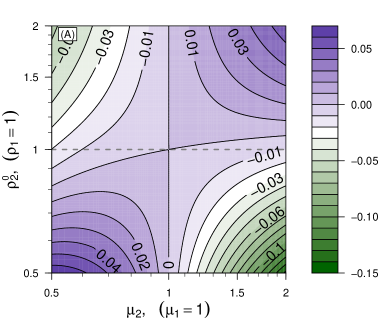
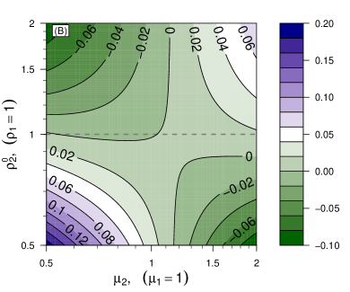
Figure 5: (color online) Panel (A), stability diagram for two solids materials with identical Poisson’s ratio of $\nu=0.25$. Panel (B), diagram for solids with Poisson’s ratios of $\nu_{1}=0.45$ and $\nu_{2}=0.40$.

IV Numerical results and discussions

The linear stability analysis revealed an intricate change in stability depending on the material properties and densities of the two solids. We explore this stability beyond the linear regime using numerical methods. The bulk elasto-static equation Eq.(13) is solved numerically on an unstructured triangular grid using the Galerkin finite element method and the surface tension force is converted to a body force in a narrow band surrounding the interface. The discontinuous jumps appearing in the dynamical Eq. (30) are computed at the outer border of the band. Periodic boundary conditions are used to minimize the possible influence of the finite system size in the x-direction (parallel to the interface). The interface is tracked using a level set method (e.g. Sethian99 ) and propagated with the normal velocity calculated in Sec. II using Eq. (30). Several level set functions, $\phi(x,t)$, can be used, however, most level set methods use the signed distance function ($|\phi(x,t)|$ is the shortest distance between $x$ and the interface and the sign of $\phi(x,t)$ identifies the phase at position $x$). Good numerical accuracy can be obtained by keeping $\phi(x,t)$ a signed distance function at all times, and this is achieved by frequent reinitialization of $\phi(x,t)$ according to the iterative scheme

$$\frac{\partial\phi}{\partial t^{\prime}}+S(\phi_{0})(|\nabla\phi|-1)=0,$$ (48)

where $\phi_{0}$ is the level set function before the reinitialization, $t^{\prime}$ is a fictitious time, and $S(\phi_{0})=\phi_{0}/\sqrt{\phi_{0}^{2}+(\Delta x)^{2}}$, where $\Delta x$ is the grid size. Generally only a couple of iterations are needed at each time step, to obtain a good approximation to a signed distance function, and it is only necessary to update the level set function in a narrow band around the interface.

In Figs. (6) and (7) we present numerical simulations of the phase transformation kinetics using parameter regions where the interface is either stable or unstable. The simulations presented in Fig. (6) panels (A) and (B) represent interface snap shots of a first order phase transition dynamics and panels (C) and (D) simulations of a second order, respectively. In panel (A), the values of the parameters were chosen in a region of the stability diagram where the interface is predicted to roughen and in panel (B) we have used parameters corresponding to a stable evolution of the interface. Note that the interface in both cases is moving from the dense phase into the soft phase independent of its stability. This is in agreement with the one dimensional calculation performed in Sec. II. Panel (C) shows a case of a second order phase transition where the interface is unstable, while panel (D) shows a stable case. We notice that, for second order phase transitions, the overall translation of the interface is changed in unison with its stability. In Eq. (46) we saw that the stability of the second order phase transition is dictated by the values of Poisson’s ratios. For Poisson’s ratio smaller than $1/3$, the kinetics is stable and the phase of small shear modulus grows into the phase of higher shear modulus while for higher values of Poisson’s ratio the behavior is reversed and the interface roughens with time. This also follows from Eq. (41). In fig. 7, we have plotted the mean velocity as a function of time for the simulations presented in fig. 6.

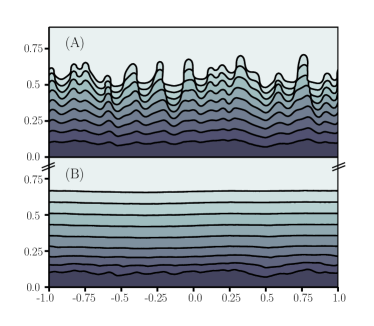
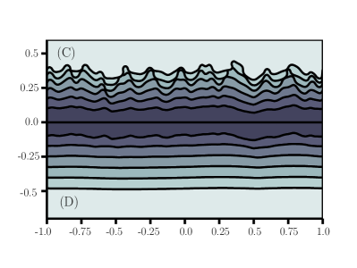
Figure 6: (color online) Simulations of the temporal evolution of solid-solid interfaces for first order (Panels (A) and (B)) and second order (Panels (C) and (D)) phase transitions. Panel (A) shows a simulation using $\rho_{1}=1.0,\mu_{1}=1.0$ and $\rho_{2}=1.05,\mu_{2}=2.0$. Both phases have identical Poisson’s ratio, $\nu_{1}=\nu_{2}=0.45$. Panel (B) is a simulation run with densities and shear modules similar to panel (A) but with a different Poisson’s ratios, $\nu_{1}=\nu_{2}=0.25$. Panel (C) is a simulation run with $\rho_{1}=1.0,\mu_{1}=1.0$ and $\rho_{2}=1.0,\mu_{2}=2.0$. Both phases have identical Poisson’s ratios, $\nu_{1}=\nu_{2}=0.45$. Panel (D) shows a simulation run with densities and shear modules similar to Panel (C) but with different Poisson’s ratios, $\nu_{1}=\nu_{2}=0.25$. The color code represents a time arrow pointing from the darker blue (early stage) to the lighter blue (final stage).

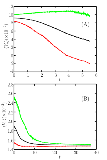
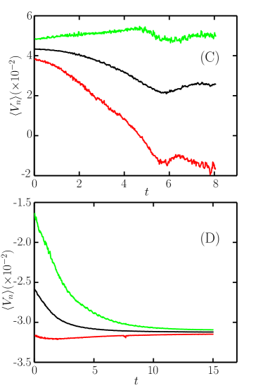
Figure 7: (color online) Normal velocity as a function of time in first order (Panels (A) and (B)) and second order (Panels (C) and (D)) phase transitions. The simulations presented in the individual panels are identical to the corresponding panels in Fig. 6. The color code of the curves reference to the mean velocity (in black), the mean of lowest $10$ % (in red) and the mean of the highest $10$ % (in green).

V Concluding remarks

In conclusion, it has been shown that the phase transformation of one solid into the another across a thin interface may lead to a morphological instability, as well as the development of fingers along the propagating interface. We have presented a stability analysis based on the Gibbs potential for non-hydrostatically stressed solids and have established a linear relationship between the rate of entropy production at the interface and the rate of mass exchange between the solid phases. The solids are compressed transverse to the interface and corresponding stability diagrams reveal an intricate dependence of the stability on the material density, Poisson’s ratio and Young’s modulus. With the density as order parameter, two types of phase transitions were considered, a first and a second order, respectively.

For both types of transitions we find expressions for the curves separating the stable and unstable regions in the stability diagram. For most material parameters the first order phase transition, i.e. when the two solids have different referential densities, destabilizes the interface by allowing fingers to grow from the denser phase into the other. When the solids have identical or almost identical densities, i.e. a second order phase transition, we find that the stability depends on Poisson’s ratios of the two solids. If the two solids have Poisson’s ratios less than 1/3, the phase transition dynamics of the two solids will lead to a flattening of the interface, i.e. any perturbation of a flat interface will decay and ultimately the interface will propagate uniformly from the soft phase (low Young’s modulus) into the hard phase (high Young’s modulus).

We believe that our classification of the phase transition order together with the stability analysis may find application in many natural systems, since the morphological stability directly provide information about the order of the underlying phase transformation process and the material parameters.

Appendix A Surface tension

In this appendix we present additional details on the derivation of the reaction rate Eq. (30) including the interfacial free energy. Let us consider a diffuse interface characterized by a small thickness over which the concentration field varies smoothly between the constant values in the bulk of the two phases. In the Cahn-Hilliard formalism, the free energy is introduced as a function of both the concentration and concentration gradients, and has the form

$$\rho\bar{f}(\bar{\epsilon}_{ij},c,\nabla c)=\rho\bar{f}_{0}(\bar{\epsilon}_{ij},c)+\frac{\kappa_{1}}{2}|\nabla c|^{2},$$ (49)

where the first term is the free energy in the bulk and the second term is associated with the interfacial free energy. Here $\kappa_{1}$ is a small parameter related to the thickness of the interface.

In this case, the calculation of the reaction rate $Q$ proceeds as in Sec. II. We apply the total time derivative of the local equilibrium equation, Eq. (16), where the free energy is given by Eq. (49) and then obtain the following expression

$$\dot{\bar{e}}=\frac{\partial\bar{f}}{\partial\bar{\epsilon}_{ij}}\dot{\overline{\epsilon_{ij}}}+\frac{\partial\bar{f}}{\partial c}\dot{c}+\frac{\partial\bar{f}}{\partial\nabla_{i}c}\left(\nabla_{i}\dot{c}-\nabla_{j}c\nabla_{i}\bar{v}_{j}\right)+T\dot{\bar{s}},$$ (50)

where the commutation relation, $\frac{d}{dt}\nabla_{i}c=\nabla_{i}\dot{c}-\nabla_{i}v_{j}\nabla_{j}c$, has been used Trusk98 . Combining the above equation with the conservation of energy from Eq. (15) and the entropy balance from Eq.(21) an expression for the entropy production rate is obtained

$$T\Pi_{s} = \left(\sigma_{ij}+\rho\nabla_{j}c\frac{\partial\bar{f}}{\partial\nabla_{i}c}\right)\nabla_{i}\bar{v}_{j}-\rho\left(\frac{\partial\bar{f}}{\partial c}-\nabla_{i}\frac{\partial\bar{f}}{\partial\nabla_{i}c}\right)\dot{c}-\rho\frac{\partial\bar{f}}{\partial\bar{\epsilon}_{ij}}\dot{\overline{\epsilon_{ij}}}$$

$$= n_{i}\left(\sigma_{ij}+\rho\nabla_{i}c\frac{\partial\bar{f}}{\partial\nabla_{j}c}\right)n_{j}Q\delta_{\Gamma}\frac{\partial}{\partial c}\left(\frac{1}{\tilde{\rho}}\right)-\left(\frac{\partial\bar{f}}{\partial c}-\nabla_{i}\frac{\partial\bar{f}}{\partial\nabla_{i}c}\right)Q\delta_{\Gamma}$$

$$+ \left(\sigma_{ij}+\rho\nabla_{i}c\frac{\partial\bar{f}}{\partial\nabla_{j}c}-\rho\frac{\partial\bar{f}}{\partial\bar{\epsilon}_{ij}}\right)\dot{\overline{\epsilon_{ij}}}.$$

We observe that $\Pi_{s}$ satisfies the second law of thermodynamics provided that the last term vanishes and the rest of the terms are brought into a quadratic form. This implies a constitutive equation for the stress given by

$$\sigma_{ij}=\rho\frac{\partial\bar{f}}{\partial\bar{\epsilon}_{ij}}-\rho\nabla_{i}c\frac{\partial\bar{f}}{\partial\nabla_{j}c},$$ (51)

and a linear kinetics law with the reaction rate being proportional to

$$Q\approx K\left(\rho\frac{\partial\bar{f}_{0}}{\partial\bar{\epsilon}_{ij}}n_{i}n_{j}\frac{\partial}{\partial c}\left(\frac{1}{\rho}\right)-\frac{\partial\bar{f}}{\partial c}+\nabla_{i}\frac{\partial\bar{f}}{\partial\nabla_{i}c}\right),$$ (52)

where $K$ is a positive local constant of proportionality and $\sigma_{ij}^{0}$ is the elastic stress in the absence of surface tension.

Using Eq. (49), the two constitutive laws may be expressed as

$$\sigma_{ij} = \sigma^{0}_{ij}-\kappa_{1}\nabla_{i}c\otimes\nabla_{j}c$$ (53)

$$Q = K\left(\sigma^{0}_{nn}\frac{\partial}{\partial c}\left(\frac{1}{\rho}\right)-\frac{\partial\bar{f}_{0}}{\partial c}+\kappa_{1}\rho^{-1}\nabla^{2}c\right),$$ (54)

where $\sigma_{ij}^{0}$ is the elastic stress obtained in Sec. II without the surface stress.

In the sharp interface limit, i.e. the thickness goes to zero, the surface free energy becomes

$$\rho f^{surf}=\kappa_{1}|\nabla c|^{2}\rightarrow\gamma\delta_{\Gamma},$$ (55)

and surface stress is related to the surface energy by

$$\sigma_{ij}^{surf}=\kappa_{1}|\nabla c|^{2}\left(1-\frac{\nabla_{i}\phi}{|\nabla\phi|}\otimes\frac{\nabla_{j}\phi}{|\nabla\phi|}\right)\rightarrow\gamma(1-n_{i}\otimes n_{j})\delta_{\Gamma}.$$ (56)

The divergence of the surface stress is then calculated as

$$\nabla_{i}\sigma^{surf}_{ij}=2\mathcal{K}\gamma n_{j}\delta_{\Gamma},$$ (57)

where $\mathcal{K}$ is the local curvature.

Appendix B Goursat functions around a perturbed flat interface

In this appendix, we explain in details how to calculate the Airy stress functions around the perturbed flat interface introduced in Sec. III. All the detailed calculations were carried out in Maple in order to handle the lengthy algebraic expressions.

The Airy stress function satisfies the biharmonic equation $\partial^{2}_{z}\partial^{2}_{\overline{z}}U=0$. This equation has a general solution which can be written in the Goursat form $U(z,\overline{z})=\Re\{\overline{z}\phi(z)+\chi(z)\}$, where $\varphi(z)$ and $\chi(z)$ are complex functions determined by the boundary conditions. Combining Eq. (39) with the Goursat solution, stress components are related to these functions by the following expressions

$$\sigma(z) = \sigma_{xx}(x,y)+\sigma_{yy}(x,y)=2\{\varphi^{\prime}(z)+\overline{\psi^{\prime}}(z)\},$$ (58)

$$\Sigma(z) = \sigma_{yy}(x,y)-\sigma_{xx}(x,y)+2i\sigma_{xy}(x,y)$$ (59)

$$= 2\{\overline{z}\varphi^{\prime\prime}(z)+\psi(z)\},$$

where $\varphi(z)=\chi^{\prime}(z)$. The solution to the biharmonic equation is determined up to a linear gauge transformation,

$$\varphi(z)\mapsto\varphi(z)+Ciz+p$$ (60)

$$\psi(z)\mapsto\psi(z)+q,$$ (61)

where $C$ is a real number and $p$, $q$ are arbitrary complex numbers.

The boundary conditions are given by the far-field stresses and the constraints at the interface. Here we consider that the system is loaded by a uniaxial compression in the y-direction, $\sigma_{yy}(x,\infty)=-|\sigma_{\infty}|<0$. Whenever the two phases are different an interface is introduced at which we require force balance and continuous displacement field. The force balance is expressed by the following jump condition

$$\left\llbracket\sigma_{xx}n_{x}+\sigma_{xy}n_{y}+i(\sigma_{yx}n_{x}+\sigma_{yy}n_{y})\right\rrbracket=-\gamma\mathcal{K}(n_{x}+in_{y}),$$

where $\mathcal{K}$ is the local curvature and $\gamma$ is the surface tension. From Eqs. (58) and (59) we find that the force balance leads to the following condition on the Goursat functions

$$\left\llbracket\varphi+z\overline{\varphi^{\prime}}+\overline{\psi}\right\rrbracket=i\int_{0}^{s}\gamma\mathcal{K}(n_{x}+in_{y})ds,$$ (62)

where $s$ is a point at the interface. The continuity of the displacement field across the interface introduces an additional jump condition given by

$$\left\llbracket\frac{1}{\mu}(-\kappa\varphi+z\overline{\varphi^{\prime}}+\overline{\psi})\right\rrbracket=0,$$ (63)

where $\mu$ is the shear modulus and $\kappa=\frac{3-\nu}{1+\nu}$ is a constant for in-plane stress-elasticity determined by the Poisson’s ratio.

The two jump conditions, Eqs. (62) and (63) combined with the far-field boundary conditions, $\varphi_{\infty}(z)=-\frac{1}{4}(1+\nu)|\sigma_{\infty}|z$ and $\psi_{\infty}(z)=-\frac{1}{2}(1-\nu)|\sigma_{\infty}|z$ are sufficient to determine the fields $\varphi_{1}(z)$, $\psi_{1}(z)$, $\varphi_{2}(z)$ and $\psi_{2}(z)$.

Superimposing an arbitrary perturbation with amplitude $h(x)$ on the flat interface, the Goursat functions are slightly altered. They can be expanded to linear order in $h(x)$ as follows Gao91 ,

$$\varphi(x) \approx \varphi_{0}(x)+ih(x)\varphi_{0}^{\prime}(x)+\Phi(x)$$ (64)

$$\psi(x) \approx \psi_{0}(x)+ih(x)\psi_{0}^{\prime}(x)+\Psi(x).$$ (65)

$\Phi(x)$ and $\Psi(x)$ are functions of $h(x)$. Inserting this expansion into Eqs. (63) and (62), we obtain that the corresponding jump conditions for the perturbation fields

$$\left\llbracket\Phi(x)+x\overline{\Phi^{\prime}}(x)+\overline{\Psi}(x)\right\rrbracket = ih(x)\left\llbracket\overline{\Sigma_{0}}(x)\right\rrbracket$$ (67)

$$+ f(x)$$

$$\left\llbracket\frac{-\kappa\Phi(x)+x\overline{\Phi^{\prime}}(x)+\overline{\Psi}(x)}{\mu}\right\rrbracket = ih(x)\left\llbracket\frac{\overline{\Sigma_{0}}(x)}{\mu}\right\rrbracket,$$ (68)

where $f(x)=i\int_{0}^{x}\gamma\mathcal{K}(n_{x}+in_{y})ds$. To linear order we find that $f(x)\approx-\gamma\int_{0}^{x}h^{\prime\prime}(s)ds$. Eqs. (67) and (68) can be rewritten equivalently as

$$\Phi_{1}(x)-\Omega\biggl{(}x\overline{\Phi^{\prime}_{1}(x)}+\overline{\Psi_{1}(x)}\biggr{)}-(1+\Lambda)\Phi_{2}(x)$$

$$=-i\Omega h(x)\overline{\Sigma}_{01}(x)+\frac{1+\Lambda}{1+\kappa}f(x)$$ (69)

$$\Phi_{2}(x)-\Pi\biggl{(}x\overline{\Phi^{\prime}_{2}(x)}+\overline{\Psi_{2}(x)}\biggr{)}-(1+\Delta)\Phi_{1}(x)$$

$$=-i\Pi h(x)\overline{\Sigma}_{02}(x)-\frac{1+\Delta}{1+\kappa}f(x).$$ (70)

The constants appearing above are expressed in terms of the elastic moduli. Adopting the notation of Gao91 , these are given by

$$\Lambda=\kappa\frac{1/\mu_{2}-1/\mu_{1}}{1/\mu_{2}+\kappa/\mu_{1}},\qquad\Pi=\frac{1/\mu_{2}-1/\mu_{1}}{\kappa/\mu_{2}+1/\mu_{1}}$$ (71)

$$\Delta=\kappa\frac{1/\mu_{1}-1/\mu_{2}}{\kappa/\mu_{2}+1/\mu_{1}},\qquad\Omega=\frac{1/\mu_{1}-1/\mu_{2}}{\kappa/\mu_{1}+1/\mu_{2}}.$$ (72)

Eqs. (69) and (70) are solved at an arbitrary point $z$ in the complex plane by applying the Cauchy integral and using the analytic continuation of each function Musk53 . Let us denote the Cauchy integral over the perturbation amplitude

$$H_{1}(z) = \frac{1}{2\pi i}\int\frac{h(x)}{x-z}dx,\textrm{ with }\Im(z)>0$$ (73)

$$H_{2}(z) = \frac{1}{2\pi i}\int\frac{h(x)}{x-z}dx,\textrm{ with }\Im(z)<0.$$ (74)

Notice that the two functions satisfy the following relations

$$\overline{H_{1}(\overline{z})}=-H_{2}(z),\qquad\overline{H_{2}(\overline{z})}=-H_{1}(z)$$

$$\Im(H_{1}(x))=\Im(H_{2}(x)),\qquad\Re(H_{1}(x))=-\Re(H_{2}(x)),$$

where the principal value of the Cauchy integral is considered when $x$ is a point on the real axis.

Thus, by applying the Cauchy integral with $\Im(z)>0$ in Eq. 69 and $\Im(z)<0$ in Eq. 70, $\Phi_{1}$ and $\Psi_{2}$ are determined in the integral form as follows

$$\Phi_{1}(z) = -i\Omega\Sigma_{0,1}H_{1}(z)+\frac{1+\Lambda}{1+\kappa}F_{1}(z)$$

$$\Phi_{2}(z) = i\Pi\Sigma_{0,2}H_{2}(z)+\frac{1+\Delta}{1+\kappa}F_{2}(z),$$

where

$$F^{\prime}(z)=\frac{1}{2\pi i}\int\frac{f^{\prime}(x)}{x-z}dx\approx-\gamma\frac{d^{2}}{dz^{2}}H(z).$$ (75)

$\Psi_{1}(z)$ is calculated from the complex conjugation of Eq. (69) when the Cauchy integral is applied on both sides of the equation and $\Im(z)>0$. In a similar manner, $\Phi_{2}(z)$ is derived from Eq. (70). The final expressions for the two functions then follow

$$\Psi_{1}(z) = -i\Sigma_{0,1}H_{1}(z)-\frac{1+\Lambda}{1+\kappa}\biggl{(}-i\Pi\Sigma_{0,2}H_{1}(z)$$

$$-\frac{1+\Delta}{1+\kappa}F_{1}(z)\biggr{)}-\frac{1+\Lambda}{\Omega(1+\kappa)}F_{1}(z)-z\Phi^{\prime}_{1}(z)$$

$$\Psi_{2}(z) = i\Sigma_{0,2}H_{2}(z)-\frac{1+\Delta}{\Pi}\biggl{(}i\Omega\Sigma_{0,1}H_{2}(z)$$

$$-\frac{1+\Lambda}{1+\kappa}F_{2}(z)\biggr{)}-\frac{1+\Delta}{\Pi(1+\kappa)}F_{2}(z)-z\Phi^{\prime}_{2}(z).$$

For a cosine perturbation of the interface, $h(x)=A\cos(kx)$, with $A\ll 1$ the Airy stress function, $U(x,y)=\Re\{\bar{z}\phi(z)+\chi(z)\}$ is obtained explicitly.

References

- (1) R. J. Asaro and W. A. Tiller, Metallurgical Transactions 3 1789, (1972)
- (2) M. A. Grinfeld, Dolk. Akad. Nauk SSSR 290, pp. 1358-1363, (1986)
- (3) H. Gao and W. D. Nix, Annu. Rev. Mater. Sci. 29, pp. 173-209 (1999)
- (4) D. J. Srolovitz, Acta Metall. 37 2, pp. 621-625, (1989)
- (5) W. Mullins, Journal of Applied Physics 28 3, (1957)
- (6) P. Meakin, Fractals, Scaling and Growth Far From Equilibrium, Cambridge University Press (1998)
- (7) P.-Y. Robin, American Mineralogist, 59, (1974).
- (8) F. C. Larche and J. W. Cahn, Acta Metallurgica, 26, pp. 1579-1589, (1978).
- (9) W. B. Kamb, Theory of preferred crystal orientation developed by crystallization under stress, J. Geol.(1958).
- (10) R. C. Fletcher, Journal of Geophysical Research, 78 32, (1973).
- (11) L. Angheluta and E. Jettestuen and J. Mathiesen and F. Renard and B. Jamtveit, Phys. Rev. Lett. 100, 096105 (2008)
- (12) J. Lowengrub and L. Truskinovsky, Proc. R. Soc. Lond. A 454, 2617 (1998).
- (13) M.E. Gurtin, Arch. Rational Mech. Anal., 123, pp. 305-335, (1993).
- (14) J. W. Cahn and J. E. Hilliard, The journal of chemical physics, 28 2, (1958).
- (15) N.I. Muskhelishvili, Some basic problems of the mathematical theory of elasticity, P. Noordhoff Ltd, Groningen-Holland (1953), 3rd edition.
- (16) J. Mathiesen, I. Procaccia and I. Regev, Phys. Rev. E 77, 026606 (2008).
- (17) H. Gao, Int. J. Solids Structures, 28 6, pp. 703-725, (1991).
- (18) J. A. Sethian, Level Set Methods and Fast Marching Methods, Cambridge, 2nd Ed. (1999).