Geometric Scaling at RHIC and LHC

Abstract

We demonstrate that the RHIC data for hadron production in $d$-$Au$ collisions for all available rapidities are compatible with geometric scaling. In order to establish the presence of scaling violations expected from small-$x$ evolution a much larger range in transverse momentum and rapidity needs to be probed. We show that the fall-off of the transverse momentum distribution of produced hadrons at LHC is a sensitive probe of small-$x$ evolution.

It is well known that the small-$x$ DIS data show geometric scaling [1]. This means that the cross section depends on $Q^{2}/Q^{2}_{s}(x)$ only, instead of $Q^{2}$ and $x$ independently, where $Q_{s}(x)$ is known as the saturation scale. Since geometric scaling arises as a feature of saturation from nonlinear evolution equations, such as the BK equation [2], its occurrence is often seen as an indication of saturation. Here, we investigate this issue by studying the scaling properties of hadron collision data from RHIC at similarly small $x$.

The small-$x$ inclusive HERA data were shown to be well described by the phenomenological Golec-Biernat Wüsthoff (GBW) model for the dipole cross section [3]. In the GBW model, the cross section is given by $\sigma=\sigma_{0}N_{\rm GBW}(r_{t},x)$, where $\sigma_{0}\simeq 23\;{\rm mb}$ and the scattering amplitude $N_{\rm GBW}$ is given by

$$N_{\rm GBW}(r_{t},x)=1-\exp\left(-\tfrac{1}{4}r_{t}^{2}Q_{s}^{2}(x)\right),$$ (1)

where $r_{t}$ is the dipole size. This amplitude depends on $r^{2}_{t}Q^{2}_{s}(x)$ only, leading to a $Q^{2}/Q^{2}_{s}(x)$ dependence of the DIS cross section. Hence, the amplitude (1) incorporates geometric scaling. The saturation scale $Q_{s}(x)$ is parameterized as

$$Q_{s}(x)=Q_{0}\,\left(\frac{x_{0}}{x}\right)^{\lambda/2},\,\quad Q_{0}=1\,\mathrm{GeV}\,$$ (2)

where $x_{0}\simeq 3\times 10^{-4}$ and $\lambda\simeq 0.3$ [1].

To investigate whether saturation may be the cause of the observed scaling, one can study geometric scaling in other experiments where similarly small values of $x$ are probed, like $d\,$-$Au$ scattering at RHIC. In terms of the dipole amplitude, the cross section of hadron production in high-energy nucleon-nucleus collisions is given by [4, 5]

$$\frac{dN_{h}}{d\,y_{h}d^{2}p_{t}}=\frac{K(y_{h})}{(2\pi)^{2}}\int_{x_{F}}^{1}dx_{1}{\frac{x_{1}}{x_{F}}}$$

$$\times\bigg{[}\sum_{q}f_{q/p}(x_{1},p_{t}^{2})N_{F}\left(\tfrac{x_{1}}{x_{F}}p_{t},x_{2}\right)D_{h/q}\left(\tfrac{x_{F}}{x_{1}},p_{t}^{2}\right)$$

$$+f_{g/p}(x_{1},p_{t}^{2})N_{A}\left(\tfrac{x_{1}}{x_{F}}p_{t},x_{2}\right)D_{h/g}\left(\tfrac{x_{F}}{x_{1}},p_{t}^{2}\right)\bigg{]}.$$ (3)

Here $N_{F}$ describes a quark scattering off the small-$x$ field of the nucleus, while $N_{A}$ applies to a gluon. The parton distribution functions $f_{q/p}$ and the fragmentation functions $D_{h/q}$ are taken at the scale $Q^{2}=p_{t}^{2}$, which we will always take to be larger than 1 GeV². The momentum fraction of the target partons equals $x_{2}=x_{1}\exp(-2y_{h})$. To good approximation one can neglect finite mass effects, i.e. equate the pseudo-rapidity $\eta$ and the rapidity $y_{h}$ and use $x_{F}=\sqrt{p_{t}^{2}+m^{2}}/\sqrt{s}\exp(\eta)\approx p_{t}/\sqrt{s}\exp(y_{h})$. Finally, there is an overall $y_{h}$-dependent $K$-factor that effectively accounts for NLO corrections. The $K$-factors are close to 1 in the forward region and become relevant towards mid-rapidity.

Unlike in DIS, in hadron-hadron collisions, a scaling dipole amplitude will not lead to a scaling property of the cross section, due to convolutions with the parton distributions and fragmentation functions in (3). Hence one cannot establish geometric scaling in the data directly, but instead one has to test the scaling properties of the dipole amplitude using a model, like the GBW model (1). However, due to its exponential fall-off at large transverse momentum, the GBW model cannot describe the RHIC data. Instead, a modification of the GBW model, which we will refer to as the DHJ model, was proposed in [4, 5]. It offers a good description of hadron production in the forward region, and is given by

$$N_{A}({q}_{t},x_{2}) \equiv \int d^{2}r_{t}\>e^{i\vec{q}_{t}\cdot\vec{r}_{t}}$$ (4)

$$\times\left[1-\exp\left(-\tfrac{1}{4}(r_{t}^{2}Q_{s}^{2}(x_{2}))^{\gamma(q_{t},x_{2})}\right)\right]~{}.$$

The corresponding expression $N_{F}$ for quarks is obtained from $N_{A}$ by the replacement $(r_{t}^{2}Q_{s}^{2})^{\gamma}\to((C_{F}/C_{A})r_{t}^{2}Q_{s}^{2})^{\gamma}$, with $C_{F}/C_{A}=4/9$. Note that the so-called “anomalous dimension” $\gamma$ is a function of $q_{t}$ rather than $r_{t}$, so that the Fourier transform can be obtained more easily.

The anomalous dimension $\gamma$ of the DHJ model is parameterized as

$$\gamma_{\rm DHJ}(q_{t},x_{2}) = \gamma_{s}$$ (5)

$$+(1-\gamma_{s})\frac{|\log(q_{t}^{2}/Q_{s}^{2}(x_{2}))|}{\lambda y+d\sqrt{y}+|\log(q_{t}^{2}/Q_{s}^{2}(x_{2}))|}.$$

Here $y=\log 1/x_{2}$ is minus the rapidity of the target partons. The saturation scale $Q_{s}(x_{2})$ and $\lambda$ are taken from the GBW model (2), including a larger value of $Q_{0}\approx 1.63\;{\rm GeV}$ to account for the size of the nucleus. The parameter $d=1.2$ was fitted to the data. Away from $Q_{s}$, $\gamma_{\rm DHJ}$ rises towards 1 like $(\log q_{t}/Q_{s})/y$; clearly the model violates geometric scaling. At the saturation scale $\gamma_{\rm DHJ}$ assumes a specific value $\gamma_{s}=0.628$. The logarithmic rise, the scaling violations and the value of $\gamma_{s}$ are expected from small-$x$ evolution [6]. However, an analysis of the BK equation suggests that a smaller value of $\gamma\approx 0.44$ may be more appropriate at $Q_{s}$ [7]. We note that the DHJ model (5) was meant to apply only outside the saturation region, which is hardly probed at RHIC. Hence the behaviour of (5) for $q_{t}<Q_{s}$ is irrelevant.

To investigate whether the RHIC data are compatible with geometric scaling, we write down a new model that features exact scaling, unlike the DHJ model. Further, the new model, which we will refer to as the GS model, does not have the logarithmic rise or the value of $\gamma$ at $Q_{s}$ that are both expected from small-$x$ evolution. Instead, it is parameterized as

$$\gamma_{\rm GS}(w=\tfrac{q_{t}}{Q_{s}})=\gamma_{1}+(1-\gamma_{1})\frac{(w^{a}-1)}{(w^{a}-1)+b}\,.$$ (6)

The parameters $a$ and $b$ will be fitted to the data. Not only is $\gamma_{\rm GS}$ exactly scaling, it also rises much faster towards 1 at large $q_{t}$ than $\gamma_{\rm DHJ}$. Expanding the exponential, we see that the large $q_{t}$ behavior of Eq.’s (5) and (6) is given by [8],

$$N_{A}({q}_{t})\stackrel{{\scriptstyle q_{t}\gg Q_{s}}}{{\propto}}\left\{\begin{array}[]{cl}\frac{Q_{s}^{2}}{q_{t}^{4}\log(q_{t}^{2}/Q_{s}^{2})}&\text{for $\gamma_{\rm DHJ}$}\\[8.61108pt] \frac{Q_{s}^{2+a}}{q_{t}^{4+a}}&\text{for $\gamma_{\rm GS}\,.$}\end{array}\right.$$ (7)

Hence, the $p_{t}$ distribution resulting from Eq. (6) will fall-off much faster than in the DHJ model. We note that our model (6) is not intended to replace other, theoretically better motivated models but is constructed simply to investigate in a general way which conclusions can really be drawn from the RHIC data in the central and forward regions.

In Fig. 1 we show $dN_{h}/(dy_{h}d^{2}p_{t})$ following from Eq. (3), calculated using the anomalous dimension $\gamma_{\rm GS}$ in combination with the amplitude (4). All $p_{t}$ distributions of produced hadrons measured at RHIC in $d$-$Au$ collisions are well described. At $Q_{s}$ we have chosen for $\gamma_{\rm GS}(w=1)=\gamma_{1}$ the same value $\gamma_{s}=0.628$ as in the DHJ model, for ease of comparison. We also use the same parameterization of $Q_{s}(x)$. We obtain the best fit of the data for $a=2.82$ and $b=168$. As mentioned, this LO analysis requires a $K$-factor to account for NLO corrections, which are expected to become more relevant towards central rapidity. The $p_{t}$-independent $K$ factors we obtain for $y_{h}=0,1,2.2,3.2,4$ are given by $K=3.4,2.9,2.0,1.6,0.7$ for our model, and $K=4.3,3.3,2.3,1.7,0.7$ for the DHJ model. For further details of the calculation see [8].

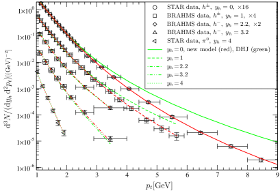
Figure 1: Transverse momentum distribution of produced hadrons in $d$-$Au$ collisions as measured at RHIC (symbols) for various rapidities $y_{h}$. To make the plot clearer, the data and the curves for $y_{h}=0,1$ and $2.2$ are multiplied with arbitrary factors, namely 16, 4 and 2, respectively.

We can conclude that the RHIC data are compatible with geometric scaling at all rapidities. Hence, no scaling violations can be claimed to be observed at RHIC. Of course, from this analysis such violations cannot be ruled out either. The fact that in the forward region where $y_{h}=2.2-4$ both the exactly scaling GS model and the scaling violating DHJ model describe the data indicates that to reach a conclusion on geometric scaling, a larger $\sqrt{s}$ is needed so that a larger range of rapidities and $p_{t}$ can be probed. Further, the logarithmic rise of $\gamma_{\rm DHJ}$ is ruled out in the central region $y_{h}=0,1$. However, the DHJ model breaks down only at mid-rapidity and $p_{t}\gtrsim 2.5$ GeV, where the values of $x_{2}$ become larger than 0.01. Even though small-$x$ evolution may not be expected to be valid anymore at $x\gtrsim 0.01$, we note that in $d\,$-$Au$ collisions at RHIC $Q_{s}$ is still larger than in DIS at $x=0.01$.

As mentioned, in the forward region both models (5) and (6) work, although they have very different properties. To illustrate how sensitive the data are to the behavior of $\gamma$, Fig. 2 shows various $\gamma_{\rm GS}(w)$’s that describe the available data equally well. All are of the form (6), with different values of $\gamma_{1}$, $a$ and $b$. The parameters that define the edges of the allowed region are $\gamma_{1}=0.50$, $a=2.60$ and $b=70.2$ for the upper curve, and $\gamma_{1}=0.75$, $a=3.10$ and $b=451$ for the lower curve. Furthermore, we add lines representing $\gamma_{\rm DHJ}$ (5) for different rapidities. To do so the rapidity of the target parton $y$ needs to be expressed in terms of $w$ and $y_{h}$, see [8] for details. As said, the region below $Q_{s}$, where the parameterization of $\gamma_{\rm DHJ}$ is not smooth, is hardly probed at RHIC. Fig. 2 shows that $\gamma$ is much more constrained by the data at large $w$ compared to the region close to $Q_{s}$. The reason for this is that around the saturation scale $r_{t}=1/Q_{s}$, the integrand in the dipole scattering amplitude (4) depends only weakly on $\gamma$. In addition, the forward data, $y_{h}=3.2$ and 4, are essentially sensitive only to $\gamma_{1}$, since for kinematic reasons they probe the region where $w$ is close to 1. Therefore, the rise of $\gamma$ with $w$ is effectively constrained only by the data for $y_{h}=0,1$. From Fig. 2 we see that $\gamma_{\rm DHJ}$ falls outside the band of allowed $\gamma$’s at large $w$, but remains inside the band for $w\lesssim 2$—this corresponds to respectively $p_{t}\gtrsim 2.5$ in the central region $y_{h}=0,1$ where the DHJ curves deviate from the data, and the entire forward region where both models work. We note that a recent study of RHIC data on the nuclear suppression factor $R^{dAu}$ suggests that the DHJ model already breaks down at $y_{h}=3.2$ [9].

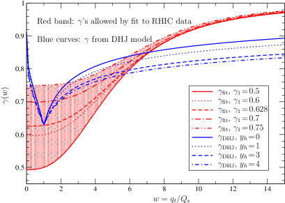
Figure 2: Various fits of $\gamma_{\rm GS}(w)$, which describe the RHIC data equally well. For comparison we show curves representing $\gamma_{\rm DHJ}(w,y(w,y_{h}))$ at different rapidities $y_{h}$.

Where the DHJ model curves deviate from the RHIC data, the probed $x_{2}$ values are not very small and one may argue that a small-$x$ description cannot be expected to apply in the first place. However, at LHC, due to the higher energies, the region of small $x_{2}$ extends to a much larger range of $p_{t}$, so that the predictions of the DHJ model and the new one will be different even at small $x_{2}$. Fig. 3 shows the $p_{t}$ distribution of hadron production in $p\,$-$Pb$ scattering at 8.8 TeV at LHC. We emphasize again that the prediction of the $p_{t}$ distribution using the GS model is to be considered a tool for checking whether certain small-$x$ properties are present in the data. For the scaling curves the best fit obtained from the RHIC data was used.

For small $p_{t}$ the predictions of the two models are comparable, since there only the region of small values of $w$ is probed where $\gamma_{\rm DHJ}$ and $\gamma_{\rm GS}$ are similar, cf. Fig. 2. Also in the very forward region, i.e. $y_{h}\approx 6-8$, only this region is tested and one obtains similar results from both models.

However, there is quite a large range where the probed values of $x_{2}$ are small but the predictions are clearly different. From Fig. 3 we see that this is the case for rapidities smaller than about 5 and $p_{t}\gtrsim 5$ GeV—this region corresponds to approximately $w\gtrsim 3$, where according to Fig. 2 the DHJ model indeed deviates from the experimentally allowed band. Due to the larger energy, the values of $x_{2}$ at LHC are much smaller than in the corresponding region of $p_{t}\gtrsim 2.5$ GeV at RHIC. At LHC, $x_{2}$ remains below 0.001 in the entire range depicted in Fig. 3, i.e. even in the central region. Hence, if the LHC data turns out to be described by the GS model, one would have a clear indication of consistency with $d\,$-$Au$ data from RHIC at forward and mid-rapidity within the small-$x$ framework of Eq. (3).

The main difference between the GS model and the DHJ model is the slope of the resulting $p_{t}$ distribution, which is directly related to the rise of $\gamma$ towards 1. Hence, a measurement of the slopes of the $p_{t}$ distribution at moderate rapidities $y_{h}$ at LHC allows a discrimination between the two models in a region where small-$x$ physics—and hence a description in terms of Eq. (3)—is expected to be applicable. The slower fall-off of the $p_{t}$ distribution in the DHJ model is caused by the logarithmic rise of $\gamma$ towards 1, which is a generic signature of small-$x$ evolution. Hence, if the $p_{t}$ distribution of the produced hadrons falls off much faster than predicted by the DHJ model, current expectations of small $x$ evolution do not hold at LHC.

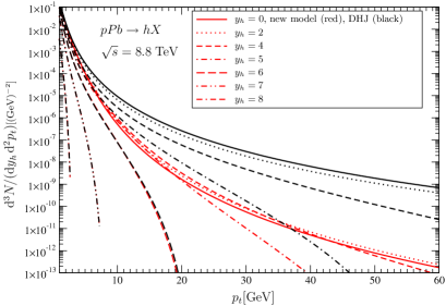
Figure 3: Hadron production cross section in $p\,$-$Pb$ collisions at LHC from $\gamma_{\rm GS}$ and $\gamma_{\rm DHJ}$ at different rapidities $y_{h}$.

References

- [1] A. M. Staśto, K. J. Golec-Biernat and J. Kwieciński, Phys. Rev. Lett. 86 (2001) 596
- [2] I. Balitsky, Nucl. Phys. B 463 (1996) 99
- [3] K. J. Golec-Biernat and M. Wüsthoff, Phys. Rev. D 59 (1999) 014017
- [4] A. Dumitru, A. Hayashigaki and J. Jalilian-Marian, Nucl. Phys. A 765 (2006) 464
- [5] A. Dumitru, A. Hayashigaki and J. Jalilian-Marian, Nucl. Phys. A 770 (2006) 57
- [6] A. H. Mueller and D. N. Triantafyllopoulos, Nucl. Phys. B 640 (2002) 331
- [7] D. Boer, A. Utermann and E. Wessels, Phys. Rev. D 75 (2007) 094022
- [8] D. Boer, A. Utermann and E. Wessels, Phys. Rev. D 77 (2008) 054014
- [9] M. A. Betemps and V. P. Goncalves, JHEP 0809 (2008) 019