Tuning of tunneling current noise spectra singularities by localized states charging

Abstract

We report the results of theoretical investigations of tunneling current noise spectra in a wide range of applied bias voltage. Localized states of individual impurity atoms play an important role in tunneling current noise formation. It was found that switching ”on” and ”off” of Coulomb interaction of conduction electrons with two charged localized states results in power law singularity of low-frequency tunneling current noise spectrum ($1/f^{\alpha}$) and also results on high frequency component of tunneling current spectra (singular peaks appear).

I Introduction

In the present work we discuss one of the possible reasons for the noise formation in the wide range of applied bias in the STM/STS junctions. Up to now the physical nature and the microscopic origin of tunneling current noise spectra formation in low and high frequency region is in general unknown. Only the limited number of works was devoted to the problem of $1/f^{\alpha}$ noise study and we have found only a few works where high frequency region of the tunneling current spectra is studied Nauen , Hohls .

We suggest the theoretical model for tunneling current noise spectra above the flat surface and above the impurity atoms on semiconductor or metallic surfaces. Our model gives an opportunity to describe not only singularities in a low frequency part of tunneling current spectra but also to reveal singular behavior of tunneling current spectra in a high frequency region and to describe spectra peculiarities in a wide range of applied bias voltage. We found experimentally that changing of tunneling current noise spectra above the flat clean surface and above the impurity atom depends on the parameters of tunneling junction such as tip-sample separation or applied bias voltage Oreshkin . Our theoretical model is rather simple, more complicated models describing noise in semiconductors can be found in Galperin -Lozano .

The investigations of the noise in two-level system was carried out in Galperin . Authors studied current noise in a double-barrier resonant-tunneling structure due to dynamic defects that switch states because of their interaction with a thermal bath. The time fluctuations of the resonant level result in low-frequency noise, the characteristics of which depend on the relative strengths of the electron escape rate and the defect’s switching rate. If the number of defects is large, the noise is of the $1/f^{\alpha}$ type. Shot noise in a mesoscopic quantum resistor is studied in Levitov . Authors found correlation functions of all order, distribution function of the transmitted charge and considered Pauli principle as the reason for the fluctuations. Current fluctuations in a mesoscopic conductor were analysed in Altshuler . Authors derived a general expression for the fluctuations in the cylindrical tunneling contact in the presence of a time dependent voltage. In Moller noise of tunneling current at zero bias voltage was investigated. It was demonstrated that at zero bias voltage the $1/f^{\alpha}$ component of noise in the tunneling current vanishes and white noise becomes dominant. The $1/f^{\alpha}$ dependence of the current noise in STM experiments on graphite in ambient conditions was investigated in Tiedje . Authors attributed this effect to fluctuations induced by adsorbates in tunneling junction area. In Lozano the fluctuations of tunneling barrier height have been investigated. The experiments have been performed under UHV conditions on graphite and gold samples using PtIr tips. From these measurements the authors have concluded that the intensity of barrier height fluctuations correspond to the intensity of tunneling current $1/f^{\alpha}$ noise in the frequency range from 1 to 100 Hz.

In our previous work we have found that for the low frequency region sudden switching on and off of additional Coulomb potential in tunneling junction area leads to typical power law dependence of tunneling current noise spectra at the threshold voltage Mantsevich . In this article our aim is to study one of the possible microscopic origins of $1/f^{\alpha}$ noise in tunneling contact in the non-resonance cases and to study high frequency peculiarities of tunneling current spectra in a wide range of applied bias voltage. We shall analise modification of tunneling current noise spectrum by the Coulomb interaction of conduction electrons in the leads (metallic tip and surface) with non-equilibrium localized charges in tunneling contact. When electron tunnels from or to localized state the Coulomb potential is suddenly switched on or off and modifies tunneling transfer amplitude. It will be shown that corrections to the tunneling vertexes caused by the Coulomb potential switching on and off result in nontrivial behavior of tunneling current noise spectrum in a wide range of applied bias voltage and should be taken in account. It was theoretically proved and observed experimentally that the same effects can lead to power law singularity in the current-voltage characteristics not only the threshold voltage but also at the high frequency region of tunneling current spectra Oreshkin .

II The suggested model and main results

We shall analyse model of two localized states in tunneling contact. In this case one of the localized states is formed by the impurity atom in semiconductor and the other one by the tip apex.

When electron tunnels in or from localized state, the electron filling numbers of localized state rapidly change leading to appearance of localized state additional charge and sudden switching ”on” and ”off” Coulomb potential. Electrons in the leads feel this Coulomb potential.

The model system (Fig. 1) can be described by hamiltonian $\hat{H}$:

$$\hat{H}=\hat{H}_{0}+\hat{H}_{tun}+\hat{H}_{int}$$

$$\hat{H}_{0} =\sum_{p}(\varepsilon_{p}-eV)c_{p}^{+}c_{p}+\sum_{k}\varepsilon_{k}c_{k}^{+}c_{k}+\sum_{i=1,2}\varepsilon_{i}a_{i}^{+}a_{i}$$

$$\hat{H}_{tun} =\sum_{k,i}T_{ki}c_{k}^{+}a_{i}+\sum_{p,i}T_{pi}c_{p}^{+}a_{i}+T\sum a_{1}^{+}a_{2}+h.c.$$

$$\hat{H}_{int} =\sum_{k,k^{{}^{\prime}}}W_{1}c_{k}^{+}c_{k^{{}^{\prime}}}a_{1}a_{1}^{+}+W_{2}c_{k}^{+}c_{k^{{}^{\prime}}}a_{2}a_{2}^{+}$$

$\hat{H}_{0}$ describes free electrons in the leads and in the localized states. $\hat{H}_{tun}$ describes tunneling transitions between the leads through localized states. $\hat{H}_{int}$ corresponds to the processes of intraband scattering caused by Coulomb potentials $W_{1}$, $W_{2}$ of localized states charges.

Operators $c_{k}^{+}(c_{k})$ and $c_{p}^{+}(c_{p})$ correspond to electrons in the leads and operators $a_{i}^{+}(a_{i})$ correspond to electrons in the localized states with energy $\varepsilon_{i}$.

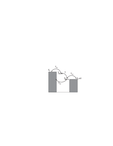
Figure 1: Schematic diagram of tunneling processes through states localized on impurity atom and on the STM tip apex.

Current noise correlation function is determined as:

$$(\hbar/e)^{2}\cdot S(t,t^{\prime})=<I_{L}(t)\cdot{I_{L}(t^{\prime})}>=$$

$$=\sum_{k,k^{{}^{\prime}},i,j}T_{k}^{2}<c_{k}^{+}(t^{\prime})a_{i}(t^{\prime})a_{j}^{+}(t)c_{k_{{}^{\prime}}}^{+}(t)>\$$

where

$$I_{L}(t)=\sum_{k}\dot{n}_{k}\cdot e=(\sum_{k}c_{k}^{+}(t^{\prime})a_{i}(t^{\prime})T_{ki}-h.c.)\cdot\frac{e}{\hbar}\$$

The current noise spectra is determined by Fourier transformation of $S(t,t^{\prime})$: $S(\omega)=\int S(\tau)d\tau\cdot e^{i\omega\tau}$. We shall use Keldysh diagram technique in our study of low frequency tunneling current noise spectra Keldysh .

Let’s consider that STM tip is a metal with a cluster on the tip apex. In this case tip apex localized state energy coincides with tip Fermi level and consequently $eV=\varepsilon_{2}$.

When we measure tunneling current spectrum above flat clean surface we deal with localized state connected with the tip. Tip apex localized state is usually formed by a cluster of several atoms or even by a single atom nearest to the surface. Tunneling transfer amplitude between the sample and the tip decreases exponentially with increasing of tip-sample separation. Thus in STM junction effective tunneling from or to the sample occurs through the atomic cluster nearest to the sample surface. So the tip apex cluster can be considered as an intermediate system for electron tunneling from the sample to the rest of the tip. Tip-sample separation is of order of interatomic distances. That’s why the electron hopping from tip apex cluster to the bulk of the tip can be also treated as tunneling process just in the same manner as it is done in tight-binding approach.

In our case of weak interaction between localized states $(T<\gamma_{k1},\gamma_{k2},\gamma_{p2})$ possible variants for localized states energy levels position in tunneling contact are: 1. impurity atom localized state energy level exceeds tip apex localized state energy level ($\varepsilon_{1}>\varepsilon_{2}=eV)$, 2. tip apex localized state energy level exceeds impurity atom localized state energy level ($\varepsilon_{2}=eV>\varepsilon_{1}$).

Expression which describes tunneling current noise spectra without Coulomb re-normalization can be calculated with the help of Keldysh diagram technic Mantsevich . It consists of three parts.

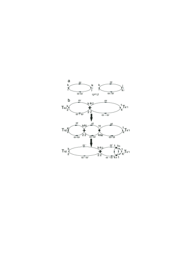
Figure 2: Lowest order diagrams contributing to tunneling current noise spectra for two localized states in tunneling contact. a) In the absence of Coulomb re-normalization of tunneling vertexes. b) In the presence of Coulomb re-normalization of tunneling vertexes. Tunneling vertexes are marked by the dot. Coulomb potential $W_{2}$ is marked by the star. Solid lines correspond to electron Green functions.

$$\widetilde{S}_{0}(\omega)=\widetilde{S}_{01}(\omega)+\widetilde{S}_{02}(\omega)+\widetilde{S}_{03}(\omega)$$

$\widetilde{S}_{01}(\omega)$ and $\widetilde{S}_{02}(\omega)$ are rather simple parts and they have the form:

$$( \hbar/e)^{2}\cdot S_{0i}(\omega)=\gamma_{ki}^{2}\cdot\int d\omega^{\prime}ImG_{ii}^{R}(\omega^{\prime})\cdot$$

$$\cdot ImG_{ii}^{R}(\omega+\omega^{\prime})\cdot(n_{i}(\omega+\omega^{\prime})-1)\cdot$$

$$\cdot (n_{i}(\omega^{\prime})-n_{k}(\omega^{\prime}))+n_{i}(\omega^{\prime})\cdot(n_{i}(\omega+\omega^{\prime})-$$

$$- n_{k}(\omega+\omega^{\prime})+\gamma_{ki}^{2}\cdot\int d\omega^{\prime}ImG_{ii}^{R}(\omega^{\prime})\cdot$$

$$\cdot ImG_{ii}^{R}(\omega+\omega^{\prime})\cdot(n_{k}(\omega+\omega^{\prime})-1)\cdot n_{i}(\omega^{\prime})-$$

$$- n_{i}(\omega^{\prime})\cdot(n_{i}(\omega+\omega^{\prime})-1)-n_{k}(\omega+\omega^{\prime})\cdot\ n_{k}(\omega^{\prime})+$$

$$+ n_{k}(\omega^{\prime})\cdot(n_{i}(\omega+\omega^{\prime})+\gamma_{ki}\cdot\int d\omega^{\prime}ImG_{ii}^{R}(\omega+\omega^{\prime})\cdot$$

$$\cdot (n_{k}(\omega^{\prime}))\cdot(n_{i}(\omega+\omega^{\prime})-1)+ImG_{ii}^{R}(\omega^{\prime})\cdot$$

$$\cdot (n_{i}(\omega^{\prime}))\cdot(n_{k}(\omega+\omega^{\prime})-1)=\widetilde{S}_{0i}\$$

where $i=1$ corresponds to the $\widetilde{S}_{01}(\omega)$ and $i=2$ corresponds to the $\widetilde{S}_{02}(\omega)$. $\widetilde{S}_{03}(\omega)$ is not trivial, it exists only due to electron tunneling transitions from one lead to both localized states. Green functions shown on the graphs are found in Maslova . The contribution of $\widetilde{S}_{01}(\omega)$ is given by graphs with $i=j=1$ (Fig. 2a), $\widetilde{S}_{02}(\omega)$ is described by graph with $i=j=2$ (Fig. 2a), $\widetilde{S}_{03}(\omega)$ is given by diagrams with $i\neq j$ (Fig. 2a).

$$( \hbar/e)^{2}\cdot S_{03}(\omega)=8\cdot\gamma_{k_{1}}\cdot\gamma_{k_{2}}\cdot\int d\omega^{\prime}ImG_{11}^{R}(\omega^{\prime})\cdot$$

$$\cdot ImG_{22}^{R}(\omega+\omega^{\prime})\cdot(n_{1}(\omega^{\prime})\cdot(n_{2}(\omega+\omega^{\prime})-1)+$$

$$+ n_{k}(\omega^{\prime})\cdot(n_{2}(\omega+\omega^{\prime})-1)+(n_{1}(\omega^{\prime})\cdot$$

$$\cdot (n_{k}(\omega+\omega^{\prime})-1)-n_{k}(\omega^{\prime})\cdot(n_{k}(\omega+\omega^{\prime})-1)+$$

$$+ 8\cdot\gamma_{k_{1}}\cdot\gamma_{k_{2}}\cdot\int d\omega^{\prime}ImG_{22}^{R}(\omega^{\prime})\cdot ImG_{11}^{R}(\omega+\omega^{\prime})\cdot$$

$$\cdot (n_{2}(\omega^{\prime})\cdot(n_{1}(\omega+\omega^{\prime})-1)+$$

$$+ n_{k}(\omega^{\prime})\cdot(n_{1}(\omega+\omega^{\prime})-1)+(n_{2}(\omega^{\prime})\cdot$$

$$\cdot (n_{k}(\omega+\omega^{\prime})-1)-n_{k}(\omega^{\prime})\cdot(n_{k}(\omega+\omega^{\prime})-1)=\widetilde{S}_{03}\$$

Some typical low frequency tunneling current noise spectra for different values of dimensionless kinetic parameters without Coulomb re normalization are shown on (Fig. 3a).

It is clearly evident that when frequency aspire to zero tunneling current spectra aspire to constant value for different dimensionless kinetic parameters. When impurity atom energy level exceeds tip apex localized state energy level ($\varepsilon_{1}>\varepsilon_{2}$) we have the largest contribution to tunneling current spectra at the high frequency range of tunneling current spectra ($\omega=\varepsilon_{2}-\varepsilon_{1}$). When tip apex localized state energy level exceeds impurity atom energy level ($\varepsilon_{2}>\varepsilon_{1}$) we have the largest contribution to tunneling current spectra at zero frequency.

Now let us consider re-normalization of the tunneling amplitude and vertex corrections to the tunneling current spectra caused by Coulomb interaction between both localized states and tunneling contact leads. Re-normalization gives us two types of diagrams contributing to the final tunneling current noise spectra expression. Ladder diagrams is the most simple type of diagrams which gives logarithmic corrections to vertexes. But this is not the only relevant kind of graphs. We must consider one more type of graphs (parquet graphs) which also gives logarithmicaly large contribution to tunneling spectra. In parquet graphs a new type of ”bubble” appears instead of ”dots” in ladder diagrams. In this situation one should retain in the n-th order of perturbation expansion the most divergent terms (Fig. 2).

It is necessary to re-normalize each vertex individually and re-normalize both vertexes jointly (Fig. 2b) Mantsevich .

The final expression for tunneling current noise spectra after Coulomb re-normalization of tunneling vertexes can be written as:

$$( \hbar/e)^{2}\cdot S(\omega)=\widetilde{S}_{0}(\omega)+\widetilde{S}_{01}(\omega)\cdot$$

$$\cdot ((\frac{D^{2}}{(\omega+eV+E_{1})^{2}+\Gamma_{2}^{2}})^{W_{1}\nu}+$$

$$+ (\frac{D^{2}}{(\omega+eV+E_{2})^{2}+\Gamma_{1}^{2}})^{W_{1}\nu})+$$

$$+ \widetilde{S}_{02}(\omega)\cdot((\frac{D^{2}}{(-\omega+eV+E_{1})^{2}+\Gamma_{1}^{2}})^{W_{2}\nu}+$$

$$+ (\frac{D^{2}}{(-\omega+eV+E_{2})^{2}+\Gamma_{2}^{2}})^{W_{2}\nu})+\widetilde{S}_{03}(\omega)\cdot$$

$$\cdot ((\frac{D^{2}}{(\omega+eV+E_{1})^{2}+\Gamma_{2}^{2}})^{W_{1}\nu}+$$

$$+ (\frac{D^{2}}{(\omega+eV+E_{2})^{2}+\Gamma_{1}^{2}})^{W_{1}\nu})\cdot$$

$$\cdot ((\frac{D^{2}}{(-\omega+eV+E_{1})^{2}+\Gamma_{1}^{2}})^{W_{2}\nu}+$$

$$+ (\frac{D^{2}}{(-\omega+eV+E_{2})^{2}+\Gamma_{2}^{2}})^{W_{2}\nu})$$

where,

$$E_{1,2} = -\frac{\varepsilon_{1}+\varepsilon_{2}}{2}\pm\frac{\sqrt{(\varepsilon_{1}-\varepsilon_{2})^{2}+4T^{2}}}{2}$$

$$\Gamma_{1} \sim \Gamma_{2}\sim(\gamma_{k2}+\gamma_{p2}+\gamma_{k1})\$$

where $D$- are the bandwidths of right and left leads, $\nu$- the equilibrium density of states in the tunneling contact leads, $W$- Coulomb potential.

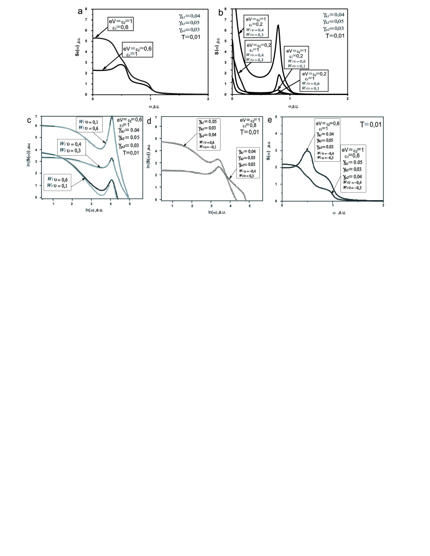
Figure 3: Typical tunneling current noise spectra for different values of dimensionless kinetic parameters for two localized states in tunneling contact ($eV=\varepsilon_{2}\neq\varepsilon_{1}$ ). a) In the absence of Coulomb re-normalization of tunneling vertexes. b) In the presence of Coulomb re-normalization of tunneling vertexes. c) In the presence of Coulomb re-normalization of tunneling vertexes in double logarithmic scale when both localized states acquire positive charge. d) In the presence of Coulomb re-normalization of tunneling vertexes in double logarithmic scale when localized states acquire charges of different signs. e). In the presence of Coulomb re-normalization of tunneling vertexes when both localized states acquire negative charge.

In the case of strong interaction between localized states in tunneling contact we have localized states energy levels splitting and as a result there is no singularity in tunneling current spectra at the low frequency region. In our situation of weak interaction between localized states $(T<\gamma_{k1},\gamma_{k2},\gamma_{p2})$ tunneling transfer amplitude $T$ plays an important role in kinetic processes in the tunneling junction but weakly influences on the energy spectra.

First of all we consider the situation when both localized states acquire positive charge. Fig. 3b demonstrate low frequency tunneling current noise spectra for typical values of dimensionless kinetic parameters. We can see that re-normalization of tunneling matrix element by switched ”on” and ”off” Coulomb potential of charged impurities leads to typical power law singularity in low frequency part of tunneling current noise spectra and to the peak in the particular high frequency region, caused by the singularity on the frequency $\omega=\varepsilon_{2}-\varepsilon_{1}$. Peak amplitude depends on kinetic parameters and on the charged localized states Coulomb potentials.

At the fixed composition of kinetic parameters maximum peak amplitude corresponds to the case when charged impurity atom localized state Coulomb potential $W_{1}$ exceeds Coulomb potential of tip apex localized state $W_{2}$. In the case of $W_{2}>W_{1}$ (Coulomb potential of charged impurity atom is larger than Coulomb potential of charged tip apex localized state) peak amplitude slightly changes by comparison with the case when Coulomb potential of charged impurity atom is similar to Coulomb potential of charged tip apex localized state $W_{1}\sim W_{2}$.

Tunneling current noise spectra in double logarithmic scale demonstrate frequency regions where every part of final expression which include different power law exponent, approximate noise spectra in the best way Fig. 3c.

Let’s analyse tunneling current spectra shown on Fig. 3c-e. In the case of two interacting positively charged localized states the tunneling current spectra at low frequency and in the region of the high frequency singularity is always determined by the term which produces the most strong of logarithmic singularity, determined by the sum of localized states Coulomb potentials at any values of dimensionless tunneling rates of tunneling contact. (Fig. 3c).

If one of the Coulomb potentials strongly exceeds the other one this potential determine tunneling current noise spectra with increasing of frequency. If Coulomb potential of charged impurity atom is similar to Coulomb potential of charged tip apex localized state $W_{1}\sim W_{2}$, tunneling current noise spectra with increasing of frequency is determined by Coulomb potential of charged tip apex state $W_{2}$ (Fig. 3c).

Let us consider tunneling current noise spectra in double logarithmic scale in the situation when localized states acquire charges of different signs Fig. 3d.

Tunneling current noise spectra in double logarithmic scale (Fig. 3d) make it clear that when localized states acquire charges of opposite signs tunneling current noise spectra in the low frequency region and in the region of the high frequency singularity ($\omega=\varepsilon_{2}-\varepsilon_{1}$) are always approximated by the term depending on maximum positive value of impurity atom Coulomb potential $W_{1}$ or tip apex localized state Coulomb potential $W_{2}$. Tunneling current noise spectra in double logarithmic scale in the situation when both localized states acquire negative charges (Fig. 3e) make it clearly evident that singular effects become negligible.

Now let’s describe interaction effects in tunneling contact when both localized states are formed by impurity atoms in the surface. In this case we can say about cluster in the surface $eV\neq\varepsilon_{2}\neq\varepsilon_{1}$.

Possible variants for localized states energy levels position in tunneling contact are:

1. applied bias voltage exceeds energy levels of both localized states in tunneling contact ($eV>\varepsilon_{2}>\varepsilon_{1}$, $eV>\varepsilon_{1}>\varepsilon_{2}$); 2. applied bias voltage exceeds energy level of one of the localized states in tunneling contact ($\varepsilon_{2}>eV>\varepsilon_{1}$, $\varepsilon_{1}>eV>\varepsilon_{2}$); 3. energy levels of both localized states in tunneling contact exceed applied bias voltage ($\varepsilon_{2}>\varepsilon_{1}>eV$, $\varepsilon_{1}>\varepsilon_{2}>eV$)

Typical low frequency tunneling current noise spectra for different values of dimensionless kinetic parameters without Coulomb re-normalization are shown on Fig. 4a.

Figure 4: Typical tunneling current noise spectra for different values of dimensionless kinetic parameters for two localized states in tunneling contact ($eV\neq\varepsilon_{2}\neq\varepsilon_{1}$). a) In the absence of Coulomb re-normalization of tunneling vertexes. b) In the presence of Coulomb re-normalization of tunneling vertexes. c) In the presence of Coulomb re-normalization of tunneling vertexes in double logarithmic scale when both localized states acquire positive charge. d)In the presence of Coulomb re-normalization of tunneling vertexes in double logarithmic scale when localized states acquire charges of different signs. e)In the presence of Coulomb re-normalization of tunneling vertexes in double logarithmic scale when both localized states acquire negative charge.

It is clearly evident that when frequency aspire to zero tunneling current spectra aspire to constant value for different dimensionless kinetic parameters. When energy levels of both localized states in tunneling contact exceeds applied bias voltage ($\varepsilon_{2}>\varepsilon_{1}>eV$ or $\varepsilon_{1}>\varepsilon_{2}>eV$) we have the largest contribution to tunneling current spectra in the high frequency region (Fig. 4a). In the other cases we have the largest contribution to tunneling current spectra at zero frequency (Fig. 4a).

Now let us consider re-normalization of the tunneling amplitude and vertex corrections to the tunneling current spectra caused by Coulomb interaction between both localized states and tunneling contact leads. Fig. 4b demonstrate tunneling current noise spectra for typical values of dimensionless kinetic parameters. It is clearly evident that when frequency aspire to zero tunneling current spectra aspire to constant value and we have no power law singularity in a low frequency part of tunneling current spectra.

We can see that re-normalization of tunneling matrix element by switched ”on” and ”off” Coulomb potential of charged impurities leads to the singular peaks in high frequency regions of tunneling current spectra, caused by singularities on the frequencies $\omega=eV-\varepsilon_{1}$ and $\omega=eV-\varepsilon_{2}$.

Let’s start from the situation when both localized states acquire positive charge. Tunneling current noise spectra in double logarithmic scale demonstrate frequency regions where every part of final expression which include different power law exponent, approximate noise spectra in the best way Fig. 4c.

Let’s analyze tunneling current spectra shown on Fig. 4c-e. In the case of two interacting positively charged localized states the tunneling current spectra in the regions of the singular peaks is determined by the term which produces the most strong of logarithmic singularity, determined by the sum of localized states Coulomb potentials at any values of dimensionless tunneling rates of tunneling contact. (Fig. 4c).

If one of the Coulomb potentials strongly exceeds the other one this potential determine tunneling current noise spectra except frequency regions in the vicinity of singular peaks . If Coulomb potentials have the similar values $W_{1}\sim W_{2}$, tunneling current noise spectra is determined by Coulomb potential of charged tip apex state $W_{2}$ (Fig. 4c).

Let us consider tunneling current noise spectra in double logarithmic scale in the situation when localized states acquire charges of different signs (Fig. 4d).

Tunneling current noise spectra in double logarithmic scale (Fig. 4d) make it clear that when localized states acquire charges of opposite signs tunneling current noise spectra is always approximated by the term depending on maximum positive value of impurity atom Coulomb potential $W_{1}$ or tip apex localized state Coulomb potential $W_{2}$.

Tunneling current noise spectra in double logarithmic scale in the situation when both localized states acquire negative charges (Fig. 4e) make it clearly evident that singular effects after Coulomb re-normalization become negligible. Simple estimation gives possibility to analyze the validity of obtained results. For typical composition of tunneling junction parameters in the low frequency region power spectrum of tunneling current corresponds to experimental results. Power spectrum on zero frequency has the form:

$$S(0)\approx(\gamma_{eff}\cdot e/\hbar)^{2}\cdot(D/\gamma_{eff1})^{\nu\cdot W}\cdot(1/\bigtriangleup\omega)$$

For typical $\gamma_{eff}$, $\gamma_{eff1}$ $\approx 10^{-13}$, $D\approx 10$, $W\approx 0,5$ $S(0)\approx 10^{-18}A^{2}/Hz$ Oreshkin .

III Conclusion

The microscopic theoretical approach describing tunneling current noise spectra in a wide range of applied bias voltage taking in account many-particle interaction was proposed. When electron tunnels to or from localized state the charge of localized state rapidly changes. This results in sudden switching on and off of additional Coulomb potential in tunneling junction area, and leads to singular behavior of tunneling current spectra in a particular frequency range determined by the parameters of tunneling junction such as applied bias voltage or the localized states energy levels deposition.

In the case of two localized states in tunneling junction when energy level of one of the localized states is connected with the tip apex and is not equal to energy level of the impurity atom localized state on the surface we can see typical power law dependence for the low frequency part of tunneling current spectra and singular peak in the particular high frequency region of tunneling current spectra determined by the localized states energy levels deposition in the tunneling junction ($eV=\varepsilon_{2}\neq\varepsilon_{1}$). In the non-resonance case of the cluster on the surface ($eV\neq\varepsilon_{2}\neq\varepsilon_{1}$) we have found two singular peaks in the high frequency region of tunneling current noise spectra. So our results demonstrate that changing of the applied bias voltage leads to the tuning of tunneling current noise spectra .

This effect can be qualitatively understood by the following way: apart from the direct tunneling from the localized state to the state with momentum $k$ in the lead of tunneling contact described by the amplitude $T_{k}$, the electron can first tunnel into any other empty state $k^{\prime}$ in the lead and then scatter to the state k by Coulomb potential. So the appearance of even a weak Coulomb potential significantly modifies the many particle wave function of the electron gas in the leads.

We are grateful to A.I. Oreshkin and S.V. Savinov for discussions and useful remarks.

This work was partially supported by RFBR grants 06-02-17076-a, 06-02-17179-a, 08-02-01020-a and the Council of the President of the Russian Federation for Support of Young Scientists and Leading Scientific School NSh-4464.2006.2.

References

- (1) A. Nauen, F. Hohls, N. Maire et al., Phys. Rev. B, 70, (2004), 033305
- (2) A. Nauen, F. Hohls, I. Hapke-Wurst et al., Phys. Rev. B, 66, (2002), 161303
- (3) A.I. Oreshkin, V.N. Mantsevich, N.S. Maslova et al., JETP Letters, 85, (2007), 46
- (4) Yu.M. Galperin, K.A. Chao, Phys. Rev. B, 55, (1995), 12126
- (5) L.S. Levitov, G.B. Lesovik, JETP Letters, 55, (1992), 534
- (6) B.L. Altshuler, L.S. Levitov, A. Yu. Yakovets, JETP Letters, 59, (1994), 821
- (7) R. Moller, A. Esslinger, B. Koslowski, Appl. Phys. Lett. 55, (1989), 2360
- (8) T. Tiedje et al. J. Vac. Sci. Technol. B, A6, (1988), 372
- (9) M. Lozano, M. Tringides, Europhys.Lett., 30, (1995), 537
- (10) V.N. Mantsevich, N.S. Maslova, Solid State Communications, 147, (2008), 278
- (11) L.V. Keldysh, Sov. Phys JETP, 20, (1964), 1018
- (12) P.I. Arseev, N.S. Maslova, V.I. Panov et al., JETP Letters, 76, (2002), 287
- (13) I.T. Dyatlov, V.V. Sudakov and K.A. Ter-Martirosian, JhETF, 5, (1957), 631
- (14) P. Nozieres, C.T. De Dominicis Phys.Rev., 178, (1969), 1097
- (15) P.I. Arseev, N.S. Maslova, V.I. Panov et al., JETP, 94, (2002), 191