The gravitational wave background from super-inflation in Loop Quantum Cosmology

Abstract

We investigate the behaviour of tensor fluctuations in Loop Quantum Cosmology, focusing on a class of scaling solutions which admit a near scale-invariant scalar field power spectrum. We obtain the spectral index of the gravitational field perturbations, and find a strong blue tilt in the power spectrum with $n_{t}\approx 2$. The amplitude of tensor modes are, therefore, suppressed by many orders of magnitude on large scales compared to those predicted by the standard inflationary scenario where $n_{t}\approx 0$.

I Introduction

A key result of the inflationary scenario of the very early universe inflation is that it gives rise to a stochastic background of gravitational wave radiation (tensor perturbations) stochastic-gw . Such a background is in principle observable and could be used to distinguish between different models of inflation distinguish . Alternative proposes such as the ekpyrotic/cyclic scenario ekpyrotic ; Boyle:2003km or phantom super-inflation phantomInflation ; Piao:2006jz lead to very different predictions for the spectral tilt of tensor perturbations when compared with the simplest inflationary models Boyle:2003km , implying the gravitational wave background could also be a powerful discriminator between competing theories. In this work we will be concerned with the gravitational wave background produced by super-inflationary scenarios within Loop Quantum Cosmology (LQC).

Loop Quantum Gravity (LQG) LQG is a background independent and non-perturbative canonical quantisation of general relativity based on Ashtekar variables: su(2) valued connections and conjugate triads. The variables used in the quantisation scheme are holonomies of the connection and fluxes of the triad. Restriction to symmetric states followed by quantisation using the techniques of LQG gives rise to LQC LQC . Although much regarding LQC is not fully understood, in particular its relation to full LQG, it has produced a number of intriguing results and resolved the problem of singular evolution present in the earlier Wheeler de Witt approach to quantum cosmology NS .

One particularly useful approach to studying the early universe in the context of LQC is that of deriving and studying effective equations of motion rho2 ; inverse ; Bojowald:2002ny ; Bojowald:2002nz ; Vandersloot:2005kh . In the context of inflation in LQC many intriguing effects have been investigated in this setting Bojowald:2002nz ; LQCinflation ; Mulryne:2006cz ; Copeland:2007qt . While such equations cannot probe fully quantum regimes, they nevertheless incorporate quantum modifications into classical evolution equations whilst avoiding the interpretational difficulties inherent in fully quantum equations. In isotropic settings two sets of modifications have been predominately considered (see Ref. Bojowald:2008ma for a discussion of other corrections which may also need to be included in certain regimes). The first originates from the spectra of quantum operators related to the inverse triad Thiemann:1996aw ; inverse , while the second arises from the use of holonomies as a basic variable in the quantisation scheme rho2 . One point to note here is that in the regime of very small scale factor, the discrete structure of space is so strong that any inhomogeneous configuration would be far from being isotropic. Therefore, despite being able to write the effective perturbation equations for a purely isotropic scenario in this regime, one should keep in mind that in reality care needs to be taken regarding the cosmological interpretation of perturbations and their evolution Bojowald:2008gw ; Bojowald:2004ax .

The two modifications have rather different origins, yet both can give rise to a period of super-inflation during which the Hubble rate rapidly increases, rather than remaining nearly constant as is the case during standard slow-roll inflation. Since the relative status of the two modifications discussed is at present unclear, most works have taken the pragmatic approach of studying the dynamics when each of the modifications is considered separately, but not including both sets of modifications simultaneously.

In earlier work Mulryne:2006cz ; Copeland:2007qt , we explored super-inflationary scalar field models in the presence of each set of modifications in turn. We worked in an approximation which neglected back-reaction, and by studying scaling, power-law solutions we derived the form of the potential required in each case for perturbations to the scalar field, produced during the super-inflationary phase, to have a scale invariant spectrum. Moreover, while the period of super-inflation in each case must be short lived, we showed that this is not a barrier for these scenarios since only a small number of e-folds of super-inflationary evolution is required to solve the horizon problem. In that work we did not, however, consider the spectrum of tensor perturbations produced by these scenarios, and this is the question to which we now turn. This question is particularly timely since the effect of the two kinds of modifications on the evolution of tensor perturbations in LQC has only recently been derived Bojowald:2007cd . The modifications have already been utilised to calculate both corrections to the gravitational wave spectrum if standard inflation occurred in the presence of LQC corrections Barrau:2008hi and the gravitational wave spectra from the ‘big bounce’ Mielczarek:2008pf which can occur in LQC.

Similar calculations have already been carried out and reported in the literature for different types of cosmologies. In particular, gravitational wave perturbations for ekpyrotic models of a collapsing universe Boyle:2003km , and for phantom superinflation scenarios Piao:2006jz have been computed. Despite being based on different physical concepts and behaviours, both cosmologies predict a strongly blue tilted spectrum of tensor perturbations, and since these have not yet been observed, it suggests that in both scenarios, the amplitude of these fluctuations are suppressed on large scales by many orders of magnitude compared to those predicted by standard inflation. This is not unexpected, as it has been pointed out in Ref. Lidsey:2004xd that a duality exists between the ekpyrotic collapse and the dynamics of a universe sourced by a phantom field. Moreover, a scale factor duality maps the ekpyrotic collapse onto the superinflationary scaling solutions in LQC Lidsey:2004uz .

Given the connections found between LQC and the ekpyrotic and phantom scenarios, one might expect that LQC also predicts a large blue tilted spectrum for the tensor perturbations. However, as the connections are at the level of the background equations and since LQC corrections also arise in the evolution equations of tensor perturbations themselves, this expectation may not be realised and a careful analysis is necessary to confirm it. We will see below that these corrections do not spoil this conjecture after all.

The structure of the paper is as follows. In Section II, we discuss the inverse triad modifications. First we review the background dynamics which give rise to a scale invariant spectrum of scalar field perturbations, and then we consider the evolution of tensor perturbations in this setting calculating their spectrum. We then repeat the exercise for holonomy corrections in section III. Finally we conclude in section IV.

II Tensor dynamics with inverse triad corrections

We first consider the cosmological equations which follow from including modifications associated with the inverse triad in LQC. This introduces two functions into the dynamics, $D_{j,l}(a)$ and $S_{j}(a)$. These functions arise because of the presence of powers of the inverse scale factor in the Hamiltonian constraint for an isotropic and homogeneous universe. A full discussion of the origin of these terms can be found in Ref. Bojowald:2002ny ; Vandersloot:2005kh (a summary can be found in appendix B of Ref. Magueijo:2007wf ), but here we simply state their basic properties. We note that we are implicitly considering either positively curved or topologically compact models. This ensures that the size of the fiducial cell does not enter in the equations of motion. $D$ and $S$ are both functions of the scale factor, and their form changes depending on the values of two ambiguity parameters: $l$ which takes values in the range $0<l<1$, and $j$ which takes half integer values. When the scale factor approaches zero, $D$ and $S$ also approach zero, whereas as $a$ increases above the critical value $a_{\star}$, which depends on $j$, they both tend to unity. As noted in the introduction, for small values of the scale factor $a\ll a_{\star}$, the assumption of isotropy may be violated. Whilst recognising the careful attention this regime deserves, and acknowledging more work is required to clarify the validity of the dynamical equations we use together with the assumption of isotropy, we hope to pave the way by demonstrating a method of calculation which can easily be employed once new light is shed on currently uncertain sections of the theory.

The unperturbed isotropic equations of motion take the form of a modified Friedmann equation

$$\mathcal{H}^{2}\equiv\left(\frac{a^{\prime}}{a}\right)^{2}=\frac{\kappa^{2}}{3}S\left(\frac{\phi^{\prime 2}}{2D}+a^{2}V(\phi)\right)\,~{},$$ (1)

where a dash represents differentiation with respect to conformal time and we have assumed that any curvature contribution has become subdominant, and the scalar field equation is

$$\phi^{\prime\prime}+2\mathcal{H}\left(1-\frac{1}{2}\frac{d\ln D}{d\ln a}\right){\phi^{\prime}}+a^{2}DV_{,\phi}=0\,.$$ (2)

For convenience, from here on we will work in units in which $\kappa^{2}=8\pi G=1$.

In this study our interest is in the evolution of tensor perturbations about this isotropic background. Tensor perturbations are defined as the transverse and trace free part of the perturbed spatial metric, and represent gravitational wave perturbations propagating on the unperturbed background spacetime. They can be further decomposed into two polarisation modes represented by $\times$ and $+$, and in LQC, with inverse triad modifications included, the equation of motion for these modes has recently been derived to be Bojowald:2007cd

$$h^{\prime\prime}_{\times,+}+2\mathcal{H}\left[1-\frac{1}{2}\frac{d\ln S}{d\ln a}\right]h^{\prime}_{\times,+}-S^{2}\nabla^{2}h_{\times,+}=0\,~{}.$$ (3)

$h_{\times,+}$ is a tensorial quantity, but from here on to avoid clutter we will drop the $\times$ and $+$ subscripts, and take $h$ to represent the magnitude of one of the polarisation modes, but always keeping in mind that both modes are present.

II.1 The background power law solution and scale invariant scalar field dynamics

In Refs. Lidsey:2004uz ; Copeland:2007qt , it was shown that in the regime $a\ll a_{\star}$ there exists a power law solution to the equations of motion (1)–(2) which is a stable attractor to the dynamics. In this regime $D(a)\approx D_{\star}a^{n}$, with $D_{\star}=\left(3/(3+2l)\right)^{3/2(1-l)}\,a_{\star}^{-n}$ and $n=3(3-l)/(1-l)$ takes values in the range $9<n<\infty$. The function $S(a)$ may be similarly approximated by $S(a)\approx S_{\star}a^{r}$, where $S_{\star}=(3/2)a_{\star}^{-r}$ and $r=3$, though we keep $r$ arbitrary in our calculations for generality. For $a\gg a_{\star}$ , $S_{\star}\approx D_{\star}\approx 1$ and $r=n=0$. The power law solution for $a\ll a_{\star}$ exists for negative power law potentials of the form $V=V_{0}\,\phi^{\beta}$ and gives rise to the dynamics

$$a(\tau) = A(-\tau)^{p}\,,$$ (4)

$$\phi^{\prime}(\tau) = -\sqrt{p\,\frac{2+(r+2)p}{\alpha}}\,\sqrt{\frac{D}{S}}\,\frac{1}{\tau}\,,$$ (5)

$$V(\tau) = \left(3-\frac{2+(r+2)p}{2\alpha}\right)\,\frac{1}{S(a\tau)^{2}}\,,$$ (6)

where for an expanding universe $\tau$ is negative and increasing towards zero. $A$ is an arbitrary normalisation constant, $\alpha=1-n/6$ with $\beta$ and $p$ being related through

$$\beta=-\frac{2}{p}\,\frac{2+(r+2)p}{n-r}\,.$$ (7)

One can expand about this solution in terms of fast roll parameters, in order to generalise the potentials which can be considered Copeland:2007qt , but here for simplicity we will consider only this exact solution.

For $-1<p<0$ the solution given above represents a universe undergoing super-inflationary evolution during which $H=\dot{a}/a$ (a dot denotes differentiation with respect to cosmic time), the Hubble rate, increases. A particularly interesting case then occurs as $p$ tends to zero from below. This represents a universe in which the scale factor is almost constant, but $H$ increases rapidly. Considering scalar field perturbations about the background field, it was shown in Refs. Mulryne:2006cz ; Copeland:2007qt , that the spectrum of scalar field perturbations attains scale invariance in this limit. Moreover, because $H$ increases so rapidly, the horizon problem is solved during this phase with only a small number of $e$-folds required. This raises the intriguing possibility that these perturbations could be responsible for the observed CMB anisotropies and hence for structure in the universe. If this were the case, no period of standard inflation in which $H$ remains nearly constant for roughly $60$ $e$-folds of expansion would be required (where number of $e$-folds is defined as $N=\ln(a/a_{\rm i})$). A natural, and indeed important question is: ‘what is the spectrum of primordial tensor perturbations which accompanies this scale invariant spectrum of scalar field perturbations?’. This is the question to which we now turn.

II.2 The primordial spectrum of tensor perturbations

To calculate the spectrum of gravitational waves produced during super-inflation we follow the standard procedure. Noting that $2a^{2}h$ is canonically conjugate to $h^{\prime}/S$ such that Bojowald:2007cd

$$\left\{\frac{1}{2S}h^{\prime}(t,x),-\frac{a^{2}}{2}\,h(t,y)\right\}=\delta^{3}(x,y)$$ (8)

the system is quantised by promoting $h$ and $h^{\prime}$ to operators and the Poisson brackets to commutators. We have

$$\left[\hat{h}^{\prime},\hat{h}\right]=-4i\frac{S}{a^{2}}\delta^{3}(x,y)\,.$$ (9)

$h$ is then decomposed into Fourier modes

$$\hat{h}=\int\frac{d^{3}k}{(2\pi)^{3/2}}\left[h_{k}(\tau)\hat{a}_{\rm\bf k}e^{i{\rm\bf k\cdot x}}+h_{k}^{*}(\tau)\hat{a}_{\rm\bf k}^{\dagger}e^{-i{\rm\bf k\cdot x}}\right]\,~{},$$ (10)

where, considering Eq. (3), we see that each mode $h_{k}$ obeys the evolution equation

$$h^{\prime\prime}_{k}+2\mathcal{H}\left(1-\frac{1}{2}\frac{d\ln S}{d\ln a}\right)h^{\prime}_{k}+S^{2}k^{2}h_{k}=0\,~{}.$$ (11)

The power spectrum for one polarisation state of tensorial fluctuations is given by the standard expression

$${\cal P}_{h}=\frac{k^{3}}{2\pi^{2}}\,\left|h_{k}\right|^{2}\,~{}.$$ (12)

In order to evaluate Eq. (12) we must solve Eq. (11). Considering the power law solution for the regime $a\ll a_{\star}$ (Eq. (4)), and using the form of $S$ in this regime, we find that Eq. (11) becomes

$$h^{\prime\prime}_{k}+2\,\frac{p}{\tau}\left(1-\frac{r}{2}\right)h^{\prime}_{k}+k^{2}S_{\star}^{2}A^{2r}(-\tau)^{2rp}h_{k}=0\,~{}.$$ (13)

which admits the exact solution

$$h_{k}(\tau)=\frac{S^{1/2}}{\mathcal{H}^{1/2}a}\sqrt{\frac{-p\,\pi}{1+rp}}\,H_{\nu}^{(1)}(x)\,,$$ (14)

where

$$\nu=\frac{1+p(r-2)}{2(1+pr)}\,,\hskip 28.45274ptx=\frac{-pSk}{(1+pr){\cal H}}\,,$$ (15)

and we have normalised the solution such that $a_{\rm\bf k}$ and $a^{\dagger}_{\rm\bf k}$ satisfy the usual raising and lowering operator algebra while $\hat{h}$ and $\hat{h}^{\prime}$ satisfy the commutation algebra (9), such that only the forward moving solution is selected in the asymptotic past (the adiabatic vacuum). The solution (14) has the expected behaviour that each $k$ mode begins in an oscillatory state where normalisation occurs, and evolves into a non-oscillatory state once each given $k$ mode crosses a suitably defined horizon. From the form of (14), it is clear that for tensor modes horizon crossing occurs when $k\approx-aH/pS$. A given mode can only be considered to become a classical perturbation once it crosses this horizon.

Taking the solution (14) and employing (12) we find that

$${\cal P}_{h}=\frac{2^{2(\nu-1)}}{\pi^{2}}\frac{\Gamma(\nu)^{2}}{\Gamma(3/2)^{2}}\left(\frac{k_{0}}{k_{\rm e}}\right)^{3-2\nu}\left(\frac{k}{k_{0}}\right)^{3-2\nu}H_{\rm e}^{2}\,,$$ (16)

We have evaluated (14) in the limit where the modes are outside the defined horizon (i.e. $x\to 0$), and have accounted for both polarisation states. The mode $k_{0}$ that corresponds to the largest scales on the CMB and $k_{\rm e}$ is defined as the last mode to cross the horizon at the end of super-inflation ($k_{\rm e}=\mathcal{H}_{\rm e}/S_{\rm e}\approx\mathcal{H}_{\rm e}$).

A couple of observations are in order. The first is that in the limit of interest, $p\to 0$, the spectrum is blue tilted with a tensor spectral index given by $n_{t}=2$, where $n_{t}$ is defined, as usual, by $P_{h}\propto k^{n_{t}}$. This implies that on large scales the spectrum is hugely suppressed. The second important point is that the magnitude of the spectrum is fixed by the Hubble rate at the end of inflation. This also fixes the magnitude of scalar perturbations and ultimately has to be normalised such that the scalar perturbations have the correct magnitude to account for the CMB anisotropies. In the scenario at hand such a normalisation is difficult to determine since the scalar field perturbations (which are close to scale invariant) must be related to curvature perturbations (as discussed at length in Refs. Copeland:2007qt ), and this step cannot be performed at present. Nevertheless in the following section we will make the reasonable assumption that $H_{\rm e}\approx 10^{-6}$ corresponding to the GUT scale in order to calculate the present-day spectrum of gravitational waves produced by this super-inflationary scenario. Furthermore, we will see that the conclusion - that the spectrum is unobservably small - is insensitive to the choice of normalisation within reasonable bounds.

II.3 The present-day spectrum

At the end of super-inflation all classical perturbations modes are outside the horizon. We will assume that reheating occurs instantaneously at the energy scale $H_{\rm e}$, and hence that the universe becomes radiation dominated at this point. Moreover we will assume the universe is classical after reheating, and any quantum corrections (similar to $D$ or $S$) are absent from the dynamics. From this point onwards modes will begin to re-enter the cosmological horizon. We schematically illustrate this dynamics in Fig. 1.

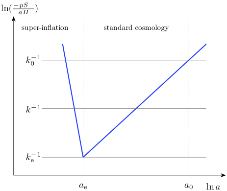
Figure 1: Schematic illustration of the evolution of modes $k$ which exit the horizon (thick solid line) during super-inflation and re-enter during the standard radiation or matter era. $k_{0}^{-1}$ is the scale corresponding to the size of the observable universe.

To convert the primordial spectrum, Eq. (16), to the spectrum which would be observed today we employ the numerically obtained transfer function Turner:1996ck ; Turner:1993vb

$$T(k)=\left(\frac{k_{0}}{k}\right)^{2}\left[1+\frac{4}{3}\frac{k}{k_{\rm eq}}+\frac{5}{2}\left(\frac{k}{k_{\rm eq}}\right)^{2}\right]^{1/2}\,,$$ (17)

where $k_{0}=H_{0}a_{0}$, is again the $k$ mode corresponding to the largest scales today, and $k_{\rm eq}=a_{\rm eq}H_{\rm eq}$, where eq stands for quantities at radiation matter equality. This form arises from the observation that tensor modes outside the horizon are roughly time independent while modes inside decay as $a^{-1}$, together with the evolution of $H\propto a^{-2}$ during radiation domination and $H\propto a^{-3/2}$ during matter domination.

Using this transfer function we can calculate the present day spectrum of tensor perturbations once we fix $H_{\rm e}$ and $k_{\rm e}/k_{0}$. A sensible estimate for $H_{\rm e}$ is the GUT scale, while an absolute upper limit is given by the Planck scale. If we also make the assumption that as many modes exit the tensor horizon as scalar modes exit the scalar horizon, $k_{0}/k_{\rm e}$ can be fixed by the requirement that the horizon problem be solved. In Ref. Copeland:2007qt we found that this required $k_{0}/k_{\rm e}\approx e^{-60}$.

A useful physical quantity that can be used to express the present day spectrum of gravitational waves is $\Omega_{\rm gw}$, the gravitational wave energy per unit logarithmic wave number in units of the critical density, $\rho_{\rm crit}=3H_{0}^{2}$, Boyle:2003km ; Turner:1996ck :

$$\Omega_{\rm gw}(k)\equiv\frac{k}{\rho_{\rm crit}}\,\frac{d\rho_{\rm gw}}{dk}=\frac{1}{6}\,\left(\frac{k}{k_{0}}\right)^{2}\,T^{2}(k)\,{\cal P}_{h}\,.$$ (18)

Figure 2 shows a plot of the present tensor abundance for a number of choices of the parameter $p$, together with the strongest observational constraints from current and future experiments searching for gravitational waves Observations .

It can be verified that even the limiting value of $H_{\rm e}\approx 1$ (giving the largest spectrum possible), leads to an unobservably small spectrum of tensor perturbations.

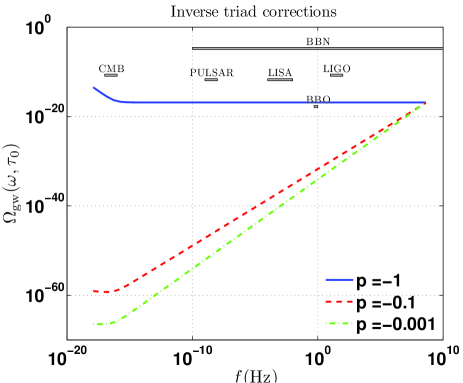
Figure 2: Predicted present abundance of gravitational waves produced during the super-inflationary phase of LQC with inverse volume corrections assuming that $H_{\rm e}=10^{-6}$ in Planck units. The solid line corresponds to the standard inflation abundance ($n=r=0$). Also indicated are the present bounds and future sensitivities.

III Tensor dynamics with holonomy corrections

We now turn our attention to the second set of effective equations, those which arise from considering that holonomies are the basic operators to be quantised in LQC.

The isotropic unperturbed dynamics is described by the Friedmann equation rho2 :

$$\mathcal{H}^{2}=\frac{1}{3}\,a^{2}\rho\,\left(1-\frac{\rho}{2\sigma}\right)\,,$$ (19)

which is modified from the classical equation by the inclusion of a $-\rho^{2}$ term, where $\sigma=3/(2\gamma^{2})$ is a constant in an exactly isotropic model, and where $\gamma$ is the Barbero-Immirzi parameter Barbero:1994ap ; Immirzi:1996di . Once again we are assuming either a flat universe or that the curvature contribution can be safely neglected. Our interest here is in a scalar field dominated universe, and hence $\rho=\phi^{\prime 2}/2a^{2}+V(\phi)$. The scalar field equation of motion remains unchanged from its classical form

$$\phi^{\prime\prime}+2\mathcal{H}\phi^{\prime}+a^{2}V_{,\phi}=0\,.$$ (20)

We stress that as we are studying inverse volume and quadratic corrections separately, we do not include the $D$ and $S$ functions in the equations of motion.

The form of the evolution equation for tensor perturbations when holonomy corrections are included has recently been derived to be Bojowald:2007cd

$$h^{\prime\prime}_{\times,+}+2\mathcal{H}h^{\prime}_{\times,+}-\nabla^{2}h_{\times,+}+T_{Q}h_{\times,+}=2\Pi_{Q}\,~{},$$ (21)

where

$$T_{Q} = \frac{a^{2}}{3}\frac{\rho^{2}}{2\sigma}\,,$$ (22)

$$\Pi_{Q} = \frac{1}{2}\,\frac{\rho}{2\sigma}\left(\frac{a^{2}}{3}\,\rho-\phi^{\prime 2}\right)\,h_{\times,+}\,,$$ (23)

are quantum corrections to the classical dynamics that become unimportant when $\rho\ll 2\sigma$. From here on we again drop the $\times$ and $+$ subscripts as we did in the inverse triad case.

III.1 Power-law solution and scale invariant scalar field perturbations

We are interested in high density regimes where $\rho$ approaches the bounding value of $2\sigma$. In this case, the term within brackets of Eq. (19) tends to zero and the behaviour of the equations alters significantly compared with the classical behaviour. Indeed in this regime we have $\dot{H}>0$ and for an expanding universe super-inflation takes place. In our previous work Copeland:2007qt , we showed that in this regime there exists an approximate power-law solution for a potential of the form $V=2\sigma-U_{0}e^{-\lambda\phi}$. Moreover, this solution is an attractor as we demonstrated both analytically and numerically Copeland:2007qt . The full solution is given by

$$a(\tau) = A(-\tau)^{p}\,,$$ (24)

$$\phi^{\prime}(\tau) = \sqrt{-2p(p+1)}\,\frac{1}{\tau}\,,$$ (25)

$$V(\tau) = 2\sigma-\frac{p(2p-1)}{(a\tau)^{2}}$$ (26)

where $A$ is an arbitrary normalisation constant. $\lambda$ and $p$ are related through

$$\lambda^{2}=-2\,\frac{p+1}{p}\,.$$ (27)

Once again $-1<p<0$ corresponds to a universe undergoing super-inflation, and moreover the limit $p\to 0$ from below leads to a scale invariant spectrum of scalar field perturbations. Furthermore, as was the case for the super-inflationary solution we studied in the presence of inverse volume corrections, only a small number of $e$-folds are required to solve the horizon problem. In our previous work we generalised the form of the potential that could be considered by expanding about this solution, but for simplicity in this work we will consider only this exact form.

We now turn our attention to the question of what spectrum of tensor perturbations accompanies the scale invariant spectrum of scalar field perturbation in this version of super-inflation.

III.2 The primordial spectrum of tensor perturbations

We again follow the standard procedure for calculating the spectrum of tensor perturbations. In this case $a^{2}h$ is canonically conjugate to $h^{\prime}$. To quantise the system $h$ and $h^{\prime}$ are promoted to operators and Fourier decomposed according to Eq. (10). Each $h_{k}$ mode satisfies the evolution equation

$$h_{k}^{\prime\prime}+2\frac{a^{\prime}}{a}\,h_{k}^{\prime}+\left[k^{2}-\frac{2p(p+1)}{\tau^{2}}\right]h_{k}=0\,,$$ (28)

during the scaling solution, where we have used $\rho\approx 2\sigma$ and Eq. (25).

The solution to Eq. (28), is given by

$$h_{k}(\tau)=\frac{1}{\mathcal{H}^{1/2}a}\sqrt{-p\,\pi}\,H_{\nu}^{(1)}(-k\tau)\,,$$ (29)

where

$$\nu=\frac{1}{2}\sqrt{1+4p+12p^{2}}\,,$$ (30)

where we have normalised the solution by the requirement that $a_{\rm\bf k}$ and $a^{\dagger}_{\rm\bf k}$ satisfy the usual raising and lowering operator algebra while $a^{2}\hat{h}$ and $\hat{h}^{\prime}$ satisfy their commutation algebra, with only the forward moving solution being selected in the asymptotic past (selecting the adiabatic vacuum). Finally, utilising Eq. (12) and evaluating this expression in the limit that the modes are outside the horizon ($k<-\mathcal{H}/p$ in this case), leads us to the same expression for the primordial power spectrum (16). The spectral index can clearly be seen to be given by $n_{t}=2$ in the limit $p\to 0$, and the amplitude fixed by $H_{\rm e}$. We note here that in cases where the dynamics of tensor perturbations could be represented by the standard equation of motion and the evolution of the scale factor is given by Eq. (24), having $p\to 0$ will inevitably result in $n_{t}=2$. This has indeed been shown to be true explicitly for the collapsing ekpyrotic scenario Boyle:2003km and for the evolution of a universe sourced by a phantom field Piao:2006jz . At this point, making some reasonable assumptions, we can proceed, as we did for the solution in the inverse triad case, to calculate the present day spectrum of gravitational wave perturbations using the transfer function Eq. (17). We show the abundance of tensors in Fig. 3 and note that the result is very similar to the inverse volume case.

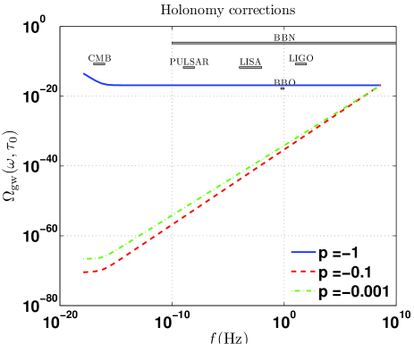
Figure 3: Predicted present abundance of gravitational waves produced during the super-inflationary phase of LQC with holonomy corrections. The solid line corresponds to the standard inflation abundance. Also indicated are the present bounds and future sensitivities.

IV Discussion

We conclude that super-inflation in both versions of the corrections in LQC predicts a strong blue spectrum of gravitational waves, hence, their abundance is strongly suppressed on the large scales and it is many orders of magnitude smaller than the value predicted in the standard inflationary scenario.

It is now important to discuss our results in the light of other investigations in the literature. In particular, it is claimed in Ref. Mielczarek:2007wc that the abundance of gravitational waves generated during super-inflation under inverse volume corrections is above the current bounds. We note however that the authors did not consider the evolution of the background in a scaling solution and the $S(a)$ correction was not used. Moreover, the full expression for the tensor perturbations was obtained more recently Bojowald:2007cd and therefore, it was not used in that work. In a more recent analysis Barrau:2008hi focusing on the holonomy corrections, it is also found, like in our work, that the spectrum of gravitational waves must be blue. However, a scaling solution was not used and the expansion of the universe was assumed to be close to de Sitter, hence, a direct comparison with our work is in fact not possible.

One needs to be cautious about making general conclusions in the context of LQC, as the theory is currently far from complete. As mentioned previously, the introduction of inhomogeneities in the small $a$ regime is likely to break the assumption of an isotropic universe. Attempts are being made to gain better understanding of this region Bojowald:2008gw . Moreover, there is the possibility that higher order perturbative correction terms could play a role, or that quantum backreaction might significantly modify the background dynamics Bojowald:2008ma .

Our work on super-inflationary scenarios in LQC also has a number of other possible drawbacks. We have treated the inverse triad and holonomy corrections separately while they should be dealt with together in a realistic set up. Though the fact that both sets of corrections lead to such similar phenomenology gives us some reassurance that combining them could lead to qualitatively similar results. Furthermore, so far we have not investigated the evolution of scalar metric perturbations. The derivation of the full equations for these is still in progress metricPerts and although these equations are not required for the calculation of tensor perturbations presented here, they are required to understand how the scale-invariant scalar field perturbation is related to the observed curvature perturbation. Finally, we should mention recent work where it has been shown that the behaviour of the LQC equations with holonomy corrections in the presence of negative exponential scalar field potentials leads to sudden singularities where the Hubble rate is bounded, but the Ricci curvature scalar diverges Cailleteau:2008wu . Given that for the case of holonomy corrections our superinflation scenario requires a scalar field potential with a negative exponential part, this serious problem needs to be avoided. In the scenarios we consider, however, the potentials only need to be of the form which gives rise to the power-law behaviour while superinflation is taking place. After this phase of evolution the potential can change in form. For example, any potential which tended to zero after the field evolved through the region which gives rise to the super-inflation phase would avoid the sudden singularity problem.

Despite the ambiguities and uncertainties in the theory, if we were to make observational claims for the scaling solutions we have considered in the current state of LQC, it would be that if gravitational waves are observed, they would rule out this scenario of superinflation in LQC sas it stands.

- (1) A. A. Starobinsky, Phys. Lett. B 91, 99 (1980); A. H. Guth, Phys. Rev. D 23, 347 (1981); A. Albrecht and P. J. Steinhardt, Phys. Rev. Lett. 48, 1220 (1982); S. W. Hawking and I. G. Moss, Phys. Lett. B 110, 35 (1982); A. D. Linde, Phys. Lett. B 108, 389 (1982); A. D. Linde, Phys. Lett. B 129, 177 (1983); A. R. Liddle and D. H. Lyth, Cosmological inflation and large-scale structure, (Cambridge University Press, 2000).
- (2) L. F. Abbott and M. B. Wise, Nucl. Phys. B 244 (1984) 541; L. F. Abbott and D. D. Harari, Nucl. Phys. B 264 (1986) 487; V. A. Rubakov, M. V. Sazhin and A. V. Veryaskin, Phys. Lett. B 115 (1982) 189; R. Fabbri and M. d. Pollock, Phys. Lett. B 125 (1983) 445.
- (3) S. Dodelson, W. H. Kinney and E. W. Kolb, Phys. Rev. D 56 (1997) 3207 [arXiv:astro-ph/9702166]; W. H. Kinney, S. Dodelson and E. W. Kolb, arXiv:astro-ph/9804034; W. H. Kinney, A. Melchiorri and A. Riotto, Phys. Rev. D 63 (2001) 023505 [arXiv:astro-ph/0007375]; W. H. Kinney, A. Melchiorri and A. Riotto, Prepared for 20th Texas Symposium on Relativistic Astrophysics, Austin, Texas, 11-15 Dec 2000; W. H. Kinney, E. W. Kolb, A. Melchiorri and A. Riotto, arXiv:0805.2966 [astro-ph].
- (4) J. Khoury, B. A. Ovrut, P. J. Steinhardt and N. Turok, Phys. Rev. D 64, 123522 (2001); J. Khoury, B. A. Ovrut, N. Seiberg, P. J. Steinhardt and N. Turok, Phys. Rev. D 65, 086007 (2002); J. Khoury, B. A. Ovrut, P. J. Steinhardt and N. Turok, Phys. Rev. D 66, 046005 (2002). P. J. Steinhardt and N. Turok, Phys. Rev. D 65, 126003 (2002); S. Gratton, J. Khoury, P. J. Steinhardt and N. Turok, Phys. Rev. D 69, 103505 (2004); J. L. Lehners, P. McFadden, N. Turok and P. J. Steinhardt, arXiv:hep-th/0702153; E. I. Buchbinder, J. Khoury and B. A. Ovrut, arXiv:hep-th/0702154; J. L. Lehners, arXiv:0806.1245 [astro-ph].
- (5) L. A. Boyle, P. J. Steinhardt and N. Turok, Phys. Rev. D 69, 127302 (2004) [arXiv:hep-th/0307170].
- (6) Y. S. Piao and E. Zhou, Phys. Rev. D 68 (2003) 083515 [arXiv:hep-th/0308080]; Y. S. Piao and Y. Z. Zhang, Phys. Rev. D 70, 063513 (2004) [arXiv:astro-ph/0401231]; Y. S. Piao and Y. Z. Zhang, Phys. Rev. D 70 (2004) 043516 [arXiv:astro-ph/0403671]; Y. S. Piao, arXiv:0706.0981 [gr-qc].
- (7) Y. S. Piao, Phys. Rev. D 73, 047302 (2006) [arXiv:gr-qc/0601115].
- (8) T. Thiemann, Introduction to modern canonical quantum general relativity, CUP, Cambridge, in press; C. Rovelli, Quantum Gravity, CUP, Cambridge, 2004; A. Ashtekar and J. Lewandowski, Class. Quant. Grav. 21 (2004) R53.
- (9) M. Bojowald, Living Rev. Rel. 8, 11 (2005); A. Ashtekar, arXiv:gr-qc/0702030.
- (10) M. Bojowald, Phys. Rev. Lett. 86, 5227 (2001).
- (11) M. Bojowald, Phys. Rev. D 64, 084018 (2001).
- (12) M. Bojowald, Class. Quant. Grav. 19, 5113 (2002).
- (13) M. Bojowald, Phys. Rev. Lett. 89, 261301 (2002).
- (14) K. Vandersloot, Phys. Rev. D 71, 103506 (2005).
- (15) A. Ashtekar, T. Pawlowski, and P. Singh, Phys. Rev. Lett. 96, 141301 (2006); A. Ashtekar, T. Pawlowski, and P. Singh, Phys. Rev. D 74, 084003 (2006); A. Ashtekar, T. Pawlowski, P. Singh, and K. Vandersloot, Phys. Rev. D75, 024035 (2007); K. Vandersloot, Phys. Rev. D75,023523 (2007); A. Corichi, T. Vukasinac, and J. A. Zapata, arXiv:0704.0007v1 [gr-qc]; P. Singh, Phys. Rev. D 73, 063508 (2006); A. Ashtekar, T. Pawlowski, P. Singh and K. Vandersloot, Phys. Rev. D 75 (2007) 024035 [arXiv:gr-qc/0612104].
- (16) S. Tsujikawa, P. Singh and R.Maartens, Class. Quant. Grav. 21, 5767 (2004); M. Bojowald, J. E. Lidsey, D. J. Mulryne, P. Singh and R. Tavakol, Phys. Rev. D 70, 043530 (2004); J. E. Lidsey, D. J. Mulryne, N. J. Nunes and R. Tavakol, Phys. Rev. D 70, 063521 (2004); D. J. Mulryne, N. J. Nunes, R. Tavakol and J. E. Lidsey, Int. J. Mod. Phys. A 20, 2347 (2005); D. J. Mulryne, R. Tavakol, J. E. Lidsey and G. F. R. Ellis, Phys. Rev. D 71, 123512 (2005); N. J. Nunes, Phys. Rev. D 72, 103510 (2005); M. Bojowald and K. Vandersloot Phys. Rev. D 67, 124023 (2003); M. Bojowald, H. Hernandez, M. Kagan, P. Singh and A. Skirzewski, Phys. Rev. Lett. 98, 031301 (2007); Phys. Rev. D 74, 123512 (2006); C. Germani, W. Nelson and M. Sakellariadou, Phys. Rev. D 76, 043529 (2007); G. M. Hossain, Class. Quant. Grav. 22, 2511 (2005); G. Calcagni and M. Cortês, Class. Quant. Grav. 24, 829 (2007).
- (17) D. J. Mulryne and N. J. Nunes, Phys. Rev. D 74, 083507 (2006).
- (18) E. J. Copeland, D. J. Mulryne, N. J. Nunes and M. Shaeri, Phys. Rev. D 77, 023510 (2008) [arXiv:0708.1261 [gr-qc]].
- (19) M. Bojowald and R. Tavakol, arXiv:0802.4274 [gr-qc].
- (20) T. Thiemann, Class. Quant. Grav. 15, 839 (1998); Class. Quant. Grav. 15, 1281 (1998).
- (21) M. Bojowald and A. Skirzewski, arXiv:0808.0701 [astro-ph].
- (22) M. Bojowald, Pramana 63 (2004) 765 [arXiv:gr-qc/0402053].
- (23) M. Bojowald and G. M. Hossain, Phys. Rev. D 77, 023508 (2008) [arXiv:0709.2365 [gr-qc]].
- (24) A. Barrau and J. Grain, arXiv:0805.0356 [gr-qc].
- (25) J. Mielczarek, arXiv:0807.0712 [gr-qc].
- (26) J. E. Lidsey, Phys. Rev. D 70, 041302 (2004).
- (27) J. E. Lidsey, JCAP 0412, 007 (2004).
- (28) J. Magueijo and P. Singh, Phys. Rev. D 76, 023510 (2007).
- (29) M. S. Turner, Phys. Rev. D 55 (1997) 435 [arXiv:astro-ph/9607066].
- (30) M. S. Turner, M. J. White and J. E. Lidsey, Phys. Rev. D 48 (1993) 4613 [arXiv:astro-ph/9306029].
- (31) T. L. Smith, E. Pierpaoli and M. Kamionkowski, Phys. Rev. Lett. 97 (2006) 021301 [arXiv:astro-ph/0603144]; L. A. Boyle and A. Buonanno, Phys. Rev. D 78 (2008) 043531 [arXiv:0708.2279 [astro-ph]]; L. A. Boyle and P. J. Steinhardt, Phys. Rev. D 77 (2008) 063504 [arXiv:astro-ph/0512014]; G. Hobbs, Class. Quant. Grav. 25 (2008) 114032 [J. Phys. Conf. Ser. 122 (2008) 012003] [arXiv:0802.1309 [astro-ph]]; J. Garcia-Bellido, D. G. Figueroa and A. Sastre, Phys. Rev. D 77 (2008) 043517 [arXiv:0707.0839 [hep-ph]].
- (32) J. F. Barbero, Phys. Rev. D 51 (1995) 5507 [arXiv:gr-qc/9410014].
- (33) G. Immirzi, Class. Quant. Grav. 14 (1997) L177 [arXiv:gr-qc/9612030].
- (34) J. Mielczarek and M. Szydlowski, arXiv:0710.2742 [gr-qc]; Phys. Lett. B 657 (2007) 20 [arXiv:0705.4449 [gr-qc]].
- (35) M. Bojowald, H. H. Hernandez, M. Kagan, P. Singh and A. Skirzewski, Phys. Rev. D 74, 123512 (2006) [arXiv:gr-qc/0609057]; M. Bojowald, G. M. Hossain, M. Kagan and S. Shankaranarayanan, arXiv:0806.3929 [gr-qc].
- (36) T. Cailleteau, A. Cardoso, K. Vandersloot and D. Wands, arXiv:0808.0190 [gr-qc].