Multi-frequency investigation of the parsec- and kilo-parsec-scale radio structures in high-redshift quasar PKS 1402$+$044

Abstract

Aims. We investigate the frequency-dependent radio properties of the jet of the luminous high-redshift ($z=3.2$) radio quasar PKS 1402$+$044 (J1405$+$0415) by means of radio interferometric observations.

Methods. The observational data were obtained with the VLBI Space Observatory Programme (VSOP) at 1.6 and 5 GHz, supplemented by other multi-frequency observations with the Very Long Baseline Array (VLBA; 2.3, 8.4, and 15 GHz) and the Very Large Array (VLA; 1.4, 5, 15, and 43 GHz). The observations span a period of 7 years.

Results. We find that the luminous high-redshift quasar PKS 1402$+$044 has a pronounced “core-jet” morphology from the parsec to the kilo-parsec scales. The jet shows a steeper spectral index and lower brightness temperature with increasing distance from the jet core. The variation of brightness temperature agrees well with the shock-in-jet model. Assuming that the jet is collimated by the ambient magnetic field, we estimate the mass of the central object as $\sim 10^{9}M_{\odot}$. The upper limit of the jet proper motion of PKS 1402$+$044 is 0.03 mas yr^-1 ($\sim 3c$) in the east-west direction.

1 Introduction

Very Long Baseline Interferometry (VLBI) studies of high-redshift quasars at a given observing frequency $\nu_{\mathrm{obs}}$ can facilitate comparison of their structural properties with those of their lower-redshift counterparts at a higher frequency, $\nu_{\mathrm{obs}}=\nu_{\mathrm{em}}/(1+z)$, where $\nu_{\mathrm{em}}$ is the emitted (rest-frame) frequency and $z$ the redshift of a distant quasar. High-redsfhit quasars provide indispensable input in all kinds of studies of the redshift-dependent properties of extragalactic objects, such as the apparent “angular size – redshift” (“$\theta$ – $z$”, e.g. Gurvits et al. gur99 (1999)) and “proper motion – redshift” (“$\mu$ – $z$”, e.g. Kellermann et al. kel99 (1999)) relations.

A statistical study of 151 quasars imaged with VLBI at 5 GHz (Frey et al. fre97 (1997)) demonstrated an overall trend of a decreasing jet-to-core flux density ratio with increasing redshift, which could be explained by the difference in spectral indices of cores and jets. Furthermore, a majority of radio QSOs at $z>4$ seemed to be even more compact than expected from the direct extrapolation of the properties of quasars at $z<4$ (Paragi et al. par99 (1999)).

A number of morphological studies of high-redshift objects have been made with the Japanese-led Space VLBI mission VSOP (VLBI Space Observatory Programme). Observations with the VSOP utilised an array consisting of a group of Earth-based radio telescopes and an 8-m space-borne antenna on board the satellite HALCA (Hirabayashi et al. hir98 (1998)). The orbiting antenna with an apogee of $\sim 21\,000$ km and perigee of $\sim 560$ km provided milli-arcsecond (mas) and sub-mas resolution at the frequencies of 1.6 and 5 GHz. VSOP observations at 1.6 GHz provided roughly the same angular resolution as Earth-based VLBI observations at 5 GHz. Thus, dual-frequency VSOP observations made it possible to map the distribution of spectral index across the source structure (e.g. Lobanov et al. lob06 (2006)) and to study frequency-dependent structural properties.

PKS 1402$+$044 (J1405$+$0415) is a flat-spectrum radio source from the Parkes 2.7-GHz Survey. In optics, it is a 19.6-magnitude ($g$ filter) stellar object at a redshift of $z=3.215$. It is a weak X-ray source with count rates of $(5.6\pm 1.2)\times 10^{-3}$ ct s^-1, over the band 0.2 – 4 keV in the Einstein IPC survey database (Thompson et al. tho98 (1998)) and $(1.3\pm 0.2)\times 10^{-2}$ ct s^-1 over the band 0.1 – 2.4 keV in the ROSAT observation (Siebert et al. sie98 (1998)). The Multi-Element Radio Linked Interferometer Network (MERLIN) observations of PKS 1402$+$044 made at 1.6 GHz indicates that there is a secondary component at a separation of $0\aas@@fstack{\prime\prime}8$ at a position angle of $-123^{\circ}$ and a faint extended emission at a distance of $3\aas@@fstack{\prime\prime}3$ at a position angle of $-106^{\circ}$. VLBI observations at 5 GHz (Gurvits et al. gur92 (1992)) found that the main component consists of a compact core and a resolved jet extending up to $\sim 18$ mas to the west.

The quasar PKS 1402$+$044 represents a relatively rare case of a strong radio source at $z>3$ and therefore a potentially rewarding target for structural studies within a broad range of angular scales. VSOP observations with their record-high angular resolution at 1.6 and 5 GHz facilitate direct comparison of structural properties of PKS 1402$+$044 with its more abundant strong radio quasars at lower redshifts at the same emitting frequency.

In this paper, we present VSOP images at 1.6 and 5 GHz, a 15-GHz Very Long Baseline Array (VLBA) image, and Very Large Array (VLA) images at 1.4, 5, 15, and 43 GHz of the quasar PKS 1402$+$044; discuss its spectral properties and brightness temperature variation along the jet; and determine some physical parameters of the core and the jet. Throughout the paper, we define the spectral index $\alpha$ as $S_{\nu}\propto\nu^{\alpha}$ and adopt the $\Lambda$CDM cosmological model (Riess et al. rie04 (2004)) with $H_{0}=75$ km s^-1 Mpc^-1, $\Omega_{\mathrm{m}}=0.3$, and $\Omega_{\Lambda}=0.7$. In the latter model, the linear scale factor for PKS 1402$+$044 is $\sim 7$ pc mas^-1.

2 Observations and data reduction

2.1 VSOP experiment

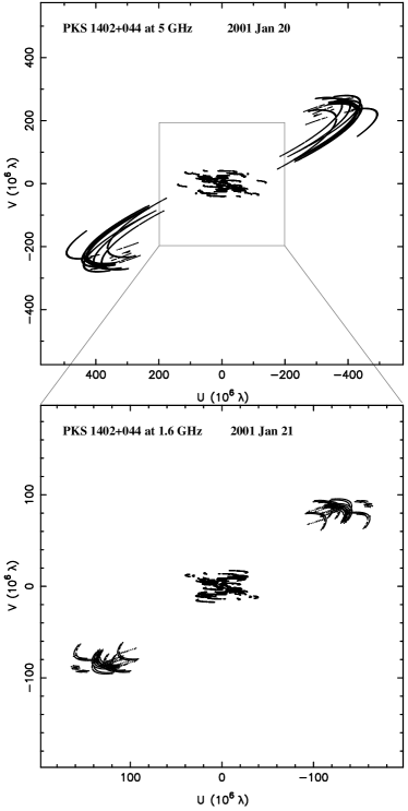
Figure 1: The effective ($u$,$v$) coverage of the VSOP observations of PKS 1402$+$044 at 1.6 GHz (bottom) and 5 GHz (top). At each frequency, the inner tracks correspond to the ground-ground baselines, and the outer tracks denote the space-ground baselines. The rectangle in the 5-GHz ($u$, $v$) coverage shows the size of the 1.6-GHz ($u$, $v$) coverage. The space-ground baselines provide $uv$-ranges roughly 2.5 – 3 times longer than ground-ground baselines.

Using the space-borne radio telescope HALCA and the VLBA, we observed the quasar PKS 1402$+$044 in left hand circular polarization at 5 GHz on 20 January 2001 and at 1.6 GHz on 21 January 2001. The observations lasted for 8 h at 1.6 GHz and 7 h at 5 GHz. The data were recorded using the VLBA tape system with a 32-MHz bandwidth consisting of 2 intermediate frequency (IF) bands and 2-bit sampling, corresponding to the data rate of 128 Mbps. Four tracking stations (Goldstone, Robledo, Tidbinbilla, Green Bank) were used to receive the HALCA downlink data. The HALCA data were recorded for $\sim$5 h at 1.6 GHz and 4.2 h at 5 GHz. The data were correlated at the VLBA correlator in Socorro with 128 spectral channels and an integration time of 4.2 s for the ground-ground baselines, and 2.1 s at 1.6 GHz, 1.0 s at 5 GHz for the space-ground baselines. In the 1.6-GHz observation, the Tidbinbilla station lost 55 minutes of space data and Green Bank lost all the space data (34 minutes) due to a problem with recording. At 5 GHz, the IF 1 data were lost for 40 minutes due to a technical malfunction at the Tidbinbilla station. Except for these problems, fringes were successfully detected on all the space-ground baselines at all times.

A priori calibration was applied for both datasets using the Astronomical Image Processing System (AIPS; Cotton cot95 (1995)). After correcting the amplitudes in cross-correlation spectrum using measurements of auto-correlation spectrum and dispersive delay due to the ionosphere from the maps of total electron content, we applied a priori amplitude calibration from the antenna gain and system temperature measurements at the Earth-based telescopes. We used the respective nominal values for HALCA. After inspecting the IF bandpass, the side channels (1 – 5, 105 – 128) in each IF were deleted because of the lower amplitude ($<80\%$) than in the centre channels. This reduced the useful observing bandwidth to 22.75 MHz. Some channels affected by radio frequency interference were flagged, too. We corrected the residual delays and rates using a two-step fringe-fitting. We first fringe-fitted the ground-array data with a solution interval of 2 minutes. Then we applied the solutions to the data, fixed the calibration for ground antennas and determined the calibration solutions of the space antenna using fringe-fitting with a 4-minute interval. After that, we combined all fringe solutions, applied them to the data, averaged all the channels in each IF, and split the multi-source data into single-source data sets. Finally, the data were exported into Difmap (Shepherd et al. she94 (1994)) and averaged further over 60 s time intervals. The hybrid imaging and self-calibration were done in Difmap. The resulting effective ($u$, $v$) coverages of the VSOP observations are shown in Fig. 1. The correlated flux densities as a function of the projected baseline length are displayed in Fig. 2, top and middle.

2.2 VLBA and VLA data

The 15-GHz VLBA data presented in this paper are from the VLBA-VSOP support survey by Gurvits et al. (in preparation). The observations were conducted on 5 December 1998 with left-hand circular polarisation, 64-MHz bandwidth and $\sim$50-minute on-source observing time. We also used the 2.3/8.6 GHz visibility data provided by US Naval Observatory (USNO) Radio Reference Frame Image Database (RRFID). Those observations used 10 VLBA antennas and some additional geodetic antennas. All the VLA data used in this paper were obtained from the NRAO Data Archive. The basic parameters of the VLA observations are summarised in Table 1. The columns give (1) frequency in GHz, (2) program ID, (3) date as dd/mm/yy, (4) array configuration, (5) antenna numbers, (6) bandwidth in MHz, and (7) total on-source time in seconds. All the VLA observations used 3C 286 as the prime flux density calibrator. After a priori calibrations in AIPS, we performed self-calibration, imaging and model-fitting in Difmap.

Table 1: VLA observations summary.

$\nu_{\mathrm{obs}}$	Program	Date	Conf.	$N_{\mathrm{ant}}$	BW	TOS
(GHz)		dd/mm/yy			(MHz)	(s)
1.4	AH0633	11/03/98	A	23	100	130
4.8	AG0670	09/10/04	A	26	100	2010
15.9	AH0633	11/03/98	A	27	100	170
43.3	AL0618	26/01/04	BC	26	100	1320

3 Results

Figure 2: Correlated flux densities of the source PKS 1402$+$044 versus ($u$, $v$) distance at 1.6 GHz (top VSOP data), 5 GHz (middle VSOP data) and 15 GHz (bottom VLBA data).

Figure 3 shows all the images of PKS 1402$+$044 of the current study. Their parameters are summarised in Table 2. The columns give: (1) frequency in GHz, (2) array and configuration, (3) weighting (NW: natural, UW: uniform), (4-5) size of the synthesised beam in mas, (6) position angle of the major axis in mas, (7) peak brightness in mJy/beam, and (8) image noise level in mJy/beam (1 $\sigma$). From the final fringe-fitted VSOP data set we produced two images: (1) an image with all data included (hereafter VSOP image) and (2) an image using only the ground VLBA data at each frequency. In the imaging process, we scaled the gridding weights inversely with the amplitude errors. The VSOP image fidelity is limited, in particular, by the completeness of the ($u$, $v$) coverage. In our case, the latter is essentially one-dimensional (see Fig. 1) that leads to a highly elliptical synthesised beam. However, luckily, the highest angular resolution is achieved along the position angle of $\sim-60^{\circ}$, very close to that of the inner pc-scale jet. Thus, the space-ground baselines obtained play an important role in imaging the inner pc-scale jet of PKS 1402$+$044.

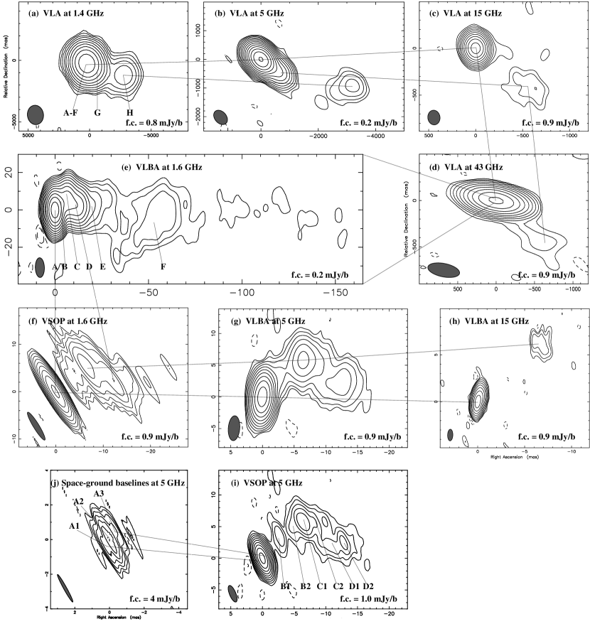
Figure 3: VLA and VLBI images of PKS 1402$+$044. The contours are drawn at $-2$, $-1$, 1, 2, …, of the respective first contour (f.c.) levels marked in the bottom of each panel. The latter are $\sim 3\sigma$ of the image thermal noise. The synthesised beams are plotted in the bottom-left corner of each image. The basic parameters of each image are listed in Table 2.

Table 2: Parameters of images in Fig. 3.

$\nu_{\mathrm{obs}}$	Array	Wt.	$b_{\mathrm{maj}}$	$b_{\mathrm{min}}$	$\theta_{\mathrm{pa}}$	$S_{\mathrm{peak}}$	$\sigma_{\mathrm{rms}}$
(GHz)			(mas)	(mas)	(∘)	(mJy/b)	(mJy/b)
1.4	VLA:A	NW	1580	1310	7.6	862	0.3
4.8	VLA:A	NW	563	404	41.7	919	0.07
15.9	VLA:A	NW	156	130	7.8	754	0.3
43.3	VLA:BC	UW	419	145	81.2	476	0.3
1.6	VLBA	NW	10.50	4.85	1.7	710	0.07
	VSOP	UW	6.88	1.19	31.7	536	0.3
4.8	VLBA	NW	3.93	1.81	$-$4.5	702	0.3
	VSOP	NW	2.79	0.99	22.3	610	0.3
	VSOP	UW	1.81	0.17	29.1	261	1.3
15.3	VLBA	NW	1.24	0.56	$-$1.7	370	0.3

We detect a very weak jet emission extending up to $\sim 150$ mas ($\sim$1 kpc) in the high dynamic range ($\sim 10\,000$) VLBA image at 1.6 GHz show Fig. 3e. It represents a typical core-jet morphology. We identify a compact core (component A) and five jet emission regions (components B – F) using circular Gaussian model-fitting in Difmap. The parameters of the models are listed in Table 3. The columns give: (1) component identification, (2) total flux density of the component, (3 - 4) radius and position angle of the centre of the component, (5) size of the fitted circular Gaussian model, (6) the smallest detectable size, and (7) brightness temperature in the source frame in K. The error ($1\sigma$) is also listed for all the values. The jet shows a wide section between 20 and 70 mas (140 – 490 pc projected distance). The uniformly-weighted VSOP image shown in Fig. 3f has a higher angular resolution (at the expense of considerably higher image noise) and indicates that components E and F are essentially resolved.

The 5-GHz VLBA image in Fig. 3g shows a similar structure to the 1.6-GHz VSOP image and the earlier 5-GHz image by Gurvits et al. (gur92 (1992)). The naturally-weighted VSOP image at 5 GHz shows that the jet components at 1.6 GHz are resolved into a few subcomponents. Here we have differentiated them with postfix number in the uniformly-weighted space-ground image (Fig. 3j). In this image, the jet appears to be heavily resolved. The core shows a three-component morphology. A weak component marked as A1 appears at the base of the jet and near the brightest component A2. The weakness of component A1 may be due to synchrotron self-absorption considering its high brightness temperature ($\sim 10^{12}$ K). There are two relatively weak jet components, B1 and B2, at 1.6 and 5 GHz between the bright components A and C. At the higher frequency, 15 GHz, both components are too weak ($<0.9$ mJy/beam) to be detected. Based on the spectrum at frequencies $\leq 5$ GHz, the extrapolated total flux density of B1$+$B2 is $\sim 5$ mJy at 15 GHz. The nondetection of the two components indicates that they have a steeper spectrum ($\alpha<-0.9$) at frequencies $>5$ GHz.

The 1.4-GHz VLA image (Fig. 3a) has the lowest resolution and shows that there is a weak ($\sim 33$ mJy) component (H) at a distance of $3\aas@@fstack{\prime\prime}22$ and a position angle $-107\aas@@fstack{\circ}4$ from the core, besides the main emission region. It agrees well with earlier MERLIN observations made with the Westerbork Synthesis Radio Telescope (WSRT; Gurvits et al. gur92 (1992)). The higher sensitivity (0.07 mJy/beam) VLA observations (Fig. 3b) at 5 GHz indicate that component H has a weak extension toward east. The extension is consistent with the hypothesis that component H belongs to the jet of PKS 1402$+$044. The main emission region can be approximated by component G and a combination of the inner components (A – F) in the VLA images. Component G is also detected at 15 GHz in Fig. 3c and even 43 GHz in Fig. 3d. The highest observing frequency corresponds to the rest-frame emitted frequency of $\sim 180$ GHz. Arguably, this is one of the rare cases of a profound jet emission at millimetre wavelengths.

Table 3: The parameters and the brightness temperatures of the fitted Gaussian models.

Comp.	$S_{\mathrm{int}}\leavevmode\nobreak\ \leavevmode\nobreak\ \leavevmode\nobreak\ \leavevmode\nobreak\$	$r$	$\theta_{\mathrm{pa}}$	$d$	$d_{\mathrm{lim}}$	$T_{\mathrm{b}}$
	(mJy)	(mas)	(∘)	(mas)	(mas)	(K)
Naturally weighted VLA image at 1.425 GHz
A-F	$795\pm 28$	0	– – –	$83\pm\ \ \ \ 2$	34	$(4.2\pm 0.3)\times 10^{8}$
G	$131\pm 12$	$701\pm 10$	$-124.5\pm 0.8$	$261\pm\ \ 21$	84	$(6.9\pm 1.3)\times 10^{6}$
H	$33\pm\ \ 8$	$3218\pm 83$	$-107.4\pm 1.5$	$691\pm 165$	167	$(2.5\pm 1.4)\times 10^{5}$
Naturally weighted VLA image at 4.860 GHz
A-F	$922\pm 33$	0	– – –	$31\pm\ \ \ \ 1$	11	$(1.0\pm 0.1)\times 10^{9}$
G	$47\pm 10$	$706\pm 25$	$-125.3\pm 2.0$	$243\pm\ \ 50$	51	$(8.3\pm 3.8)\times 10^{5}$
H	$4\pm\ \ 2$	$3324\pm 68$	$-106.1\pm 1.2$	$430\pm 136$	98	$(2.5\pm 1.8)\times 10^{4}$
Naturally weighted VLA image at 14.94 GHz
A-F	$756\pm 35$	0	– – –	$7\pm\ 0.5$	4	$(5.7\pm 0.5)\times 10^{9}$
G	$15\pm\ \ 5$	$704\pm 48$	$-126.6\pm 3.9$	$282\pm\ \ 96$	25	$(6.5\pm 5.0)\times 10^{4}$
Uniformly weighted VLA image at 43.34 GHz
A-F	$477\pm 17$	0	– – –	$4\pm\ 0.2$	12	$(3.0\pm 0.2)\times 10^{9}$
G	$6\pm\ \ 2$	$698\pm 52$	$-127.8\pm 4.3$	$277\pm 103$	109	$(8.6\pm 7.4)\times 10^{3}$
Naturally weighted VLBA image at 1.646 GHz
A	$713\pm 38$	0	– – –	$0.77\pm 0.03$	0.25	$(3.8\pm 0.4)\times 10^{12}$
B	$35\pm\ \ 8$	$4.88\pm 0.11$	$-43.7\pm 1.3$	$1.20\pm 0.23$	0.96	$(7.5\pm 3.3)\times 10^{10}$
C	$98\pm 12$	$8.81\pm 0.12$	$-50.2\pm 0.8$	$2.70\pm 0.24$	0.57	$(4.2\pm 0.9)\times 10^{10}$
D	$68\pm 10$	$12.32\pm 0.23$	$-79.8\pm 1.1$	$3.92\pm 0.47$	0.68	$(1.4\pm 0.4)\times 10^{10}$
E	$13\pm\ \ 6$	$19.32\pm 2.07$	$-84.6\pm 6.1$	$9.14\pm 4.14$	1.60	$(4.7\pm 4.6)\times 10^{8}$
F	$14\pm\ \ 8$	$55.32\pm 5.58$	$-94.2\pm 5.8$	$20.82\pm 11.2$	1.50	$(1.0\pm 0.9)\times 10^{8}$
Naturally weighted VSOP image at 4.862 GHz
A1	$134\pm 12$	0	– – –	$0.18\pm 0.01$	0.10	$(4.4\pm 0.8)\times 10^{12}$
A2	$454\pm 21$	$0.49\pm 0.01$	$-25.6\pm 0.9$	$0.29\pm 0.01$	0.05	$(5.7\pm 0.5)\times 10^{12}$
A3	$144\pm 12$	$1.10\pm 0.01$	$-29.1\pm 0.8$	$0.41\pm 0.03$	0.09	$(8.9\pm 1.4)\times 10^{11}$
B1	$10\pm\ \ 4$	$4.58\pm 0.11$	$-37.4\pm 1.4$	$0.66\pm 0.22$	0.35	$(2.5\pm 1.9)\times 10^{10}$
B2	$4\pm\ \ 2$	$6.65\pm 0.15$	$-41.7\pm 1.3$	$0.66\pm 0.29$	0.57	$(9.7\pm 9.5)\times 10^{9}$
C1	$52\pm\ \ 9$	$9.12\pm 0.13$	$-46.4\pm 0.8$	$1.64\pm 0.26$	0.15	$(2.0\pm 0.8)\times 10^{10}$
C2	$14\pm\ \ 5$	$10.78\pm 0.37$	$-54.1\pm 2.0$	$2.21\pm 0.73$	0.30	$(3.1\pm 2.3)\times 10^{9}$
D1	$8\pm\ \ 3$	$10.11\pm 0.35$	$-73.4\pm 2.0$	$1.84\pm 0.69$	0.39	$(2.6\pm 2.2)\times 10^{9}$
D2	$26\pm\ \ 8$	$13.18\pm 0.38$	$-78.0\pm 1.6$	$2.52\pm 0.76$	0.22	$(4.3\pm 2.9)\times 10^{9}$
Naturally weighted VLBA image at 15.34 GHz
A1	$102\pm 13$	0	– – –	$0.21\pm 0.02$	0.07	$(7.7\pm 1.8)\times 10^{11}$
A2	$287\pm 21$	$0.50\pm 0.01$	$-19.5\pm 1.3$	$0.18\pm 0.01$	0.04	$(2.9\pm 0.4)\times 10^{12}$
A3	$207\pm 18$	$1.24\pm 0.02$	$-20.9\pm 0.9$	$0.52\pm 0.03$	0.05	$(2.6\pm 0.5)\times 10^{11}$
C1	$29\pm\ \ 9$	$9.58\pm 0.23$	$-46.0\pm 1.4$	$1.64\pm 0.47$	0.14	$(3.6\pm 2.3)\times 10^{9}$

4 Discussion

4.1 Spectral properties of the jet

The resolution ($6.88\times 1.19$ mas) of the Space VLBI image of PKS 1402$+$044 at 1.6 GHz is close ($3.55\times 1.40$ mas) to that of the ground VLBA image at 5 GHz, enabling extraction of spectral index information from a combination of the two images. We restored the 1.6-GHz VSOP image and the 5-GHz VLBA image with a circular Gaussian beam of 4 mas in diameter. The artificial beam increases the beam area by a factor of $\sim 2$ at 1.6 GHz and $\sim 3$ at 5 GHz compared to the areas of the original synthesised beams. Both images were aligned at the strongest component. The shifts in the image centre are less than 0.1 mas ($\ll$ 4-mas resolution). After the alignment, the spectral index was calculated at all pixels with brightness values higher than 1.8 mJy/beam ($5\sigma$) in the 1.6-GHz image and 1.2 mJy/beam ($5\sigma$) in the 5-GHz image. A possible core shift between the two frequencies as predicted by Kovalev et al. (kov08 (2008)) does not exceed 1.5 mas. Thus, it does not affect the large-scale spectral distribution.

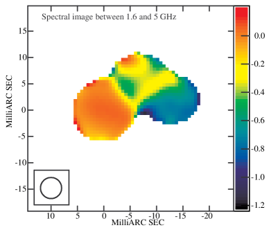
Figure 4: The spectral index distribution in the jet of the quasar PKS 1402$+$044.

The final spectral index distribution between 1.6 GHz and 5 GHz is displayed in Fig. 4. It shows a smooth distribution of spectral index on $\sim 20$ mas (140 pc) scale. The spectral index varies from $+$0.1 in the optically thick base region to $-1.0$ in the optically thin regions on the western side. To further confirm the variation, we plotted the components spectra in Fig. 5. Here we also used the 2.3/8.4-GHz visibility data from the USNO RRFID database. We fitted the VLBI visibility data with three components at each frequency (1.6, 2.3, 5, 8.4, and 15 GHz). The spectra of the large-scale components G and H are also plotted. All spectra can be approximated by a power-law model, $S_{\nu}=S_{0}\nu^{\alpha}$. The spectral indices are listed in Table 4. The spectral steepening increases with the increase in the distance from the core. The spectral difference is 0.47 between components A and B$+$C and reaches 1.57 between component A and the farthest component H. This spectral index gradient results in the variation in the flux density ratio of the components (B+C) over A from $\sim 0.19$ at 1.6 GHz to $\sim 0.05$ at 15 GHz. In a sample of sources at various redshifts, an increase in redshift is equivalent to the increase in the intrinsic emitting frequency, $\nu_{\mathrm{em}}=\nu_{\mathrm{obs}}(1+z)$. Thus, a decrease in jet-to-core flux density ratio with increase in redshift is expected (Frey et al. fre97 (1997)). The quasar PKS 1402$+$044 has a spectral difference of $\sim 0.6$ at the pc scale, which agrees well with the prediction $0.55\pm 0.43$ by Frey et al. (fre97 (1997)).

Figure 5: The component spectra in the jet of the quasar PKS 1402$+$044. The dotted lines represent the fitted curves with the simple power-law model $S_{\nu}=S_{0}\nu^{\alpha}$. The estimated spectral indices are listed in Table 4.

Table 4: Results of the power-law spectral model fits for each component shown in Fig. 5.

Comp.	$S_{0}$	$\alpha$	$\chi^{2}$
	(Jy)
A	$0.79\pm 0.05$	$-0.09\pm 0.04$	1.19
B+C	$0.17\pm 0.02$	$-0.56\pm 0.10$	0.72
D	$0.12\pm 0.02$	$-0.83\pm 0.19$	0.16
G	$0.18\pm 0.09$	$-0.91\pm 0.09$	0.08
H	$0.06\pm 0.03$	$-1.66\pm 0.40$	- - -

4.2 The mass of the central object of PKS 1402$+$044

The richness of the core-jet morphology in PKS 1402$+$044 makes it a suitable source for estimating parameters of the central black hole. The smallest detectable size for a circular Gaussian component in an image with an rms noise $\sigma_{\mathrm{rms}}$ is defined as (Lobanov lob05 (2005)):

$$d_{\mathrm{lim}}=\frac{2^{2-\beta/2}}{\pi}\left[\pi\leavevmode\nobreak\ b_{\mathrm{maj}}\leavevmode\nobreak\ b_{\mathrm{min}}\ln 2\ln\left(\frac{S_{\mathrm{int}}/\sigma_{\mathrm{rms}}}{S_{\mathrm{int}}/\sigma_{\mathrm{rms}}-1}\right)\right]^{1/2},$$ (1)

where $S_{\mathrm{int}}$ is the integrated flux density of the component, $b_{\mathrm{maj}}$ and $b_{\mathrm{min}}$ are the major and minor axes of the restoring beam respectively, $\beta=0$ for uniform weighting and $\beta=2$ for naturally weighting. Based on the above criterion, except for the size of the combined component from A to F at 43 GHz, all the sizes estimated from our VLBI and VLA images in Column (5) of Table 3 can be taken as the true sizes of the jet emission regions.

If the component size is related to the physical transverse dimension of the jet, the mass of the central object can be estimated assuming that the jet is collimated by the ambient magnetic field of the host galaxy. The jet components A2 and A3 have the best measurements of the width of the jet close to the central object, as they are most likely free of the effect of the adiabatic expanding of the jet and synchrotron self-absorption and have the higher reliability, $d/\sigma_{d}>10$, where $d$ and $\sigma_{d}$ are the angular size and error of the fitted circular Gaussian component. For a jet collimated by the ambient magnetic field $B_{\mathrm{ext}}$ of the host galaxy, the mass of the central object $M_{\mathrm{BH}}$ can be related to the width of the jet $r_{\mathrm{jet}}$ (in pc) according to the following relation (Beskin bes97 (1997)):

$$M_{\mathrm{BH}}\simeq r_{\mathrm{jet}}(B_{\mathrm{ext}}/B_{\mathrm{gr}})^{1/2}10^{13}M_{\odot},$$ (2)

where $B_{\mathrm{gr}}$ is the magnetic field measured at the Schwarzschild radius $R_{\mathrm{gr}}$ of the central black hole. Equation (2) refers to the transverse dimension of the jet measured at distances comparable to the collimation scale (typically expected to be located at $10^{2}$ – $10^{3}\leavevmode\nobreak\ R_{\mathrm{gr}}$). A typical galactic magnetic field is $B_{\mathrm{ext}}\sim 10^{-5}$ G (Beck bec00 (2000)) and one can expect to have $B_{\mathrm{gr}}\sim 10^{4}$ G (Field & Rogers fie93 (1993)). Based on these parameters, the mass of the central object is $\sim 10^{9}M_{\odot}$. The main uncertainty of the mass estimation arises from the uncertainty in $B_{\mathrm{gr}}$. However, the dependence of the mass on the value $B_{\mathrm{gr}}$ is rather weak, $M_{\mathrm{BH}}\propto B_{\mathrm{gr}}^{-0.5}$; with the magnetic field varying within 4 orders of magnitude, the estimated central black hole mass varies within two orders of magnitude. The external magnetic field $B_{\mathrm{ext}}$ normally varies within a narrow range around ($10^{-5\pm 1}$ G). Thus, the magnetic field uncertainty should not affect the estimated mass drastically.

4.3 Brightness temperature

Based on the parameters of the Gaussian models listed in Table 2, we calculated the brightness temperature of each component using the following formula (Kellermann & Owen kel88 (1988)):

$$T_{\mathrm{b}}=1.22\times 10^{12}(1+z)\frac{S_{\mathrm{int}}}{d^{2}\nu^{2}},$$ (3)

where $S_{\mathrm{int}}$ is the integrated flux density in Jy, $d$ the size of a circular Gaussian component in mas, and $\nu$ the observing frequency in GHz. The estimated brightness temperatures are listed in the last column of Table 2. Among these components, the component A2 has the highest brightness temperature, $T_{\mathrm{B}}=(5.7\pm 0.5)\times 10^{12}$ K, which is somewhat higher than the inverse Compton limit ($\sim 10^{12}$ K; Kellermann & Pauliny-Toth kel69 (1969)) but still 10-times lower than the currently known highest value of $5.8\times 10^{13}$ K found in the BL Lac object AO 0235$+$164 by Frey et al. (fre00 (2000)). In the equipartition jet model of Blandford & Königl (bla79 (1979)), the limiting brightness temperature is about $3\times 10^{11}\delta^{5/6}$ K, where $\delta$ is the Doppler factor. Comparing the theoretical value with the estimated brightness temperature of the component A2, we can obtain a conservative lower limit to the Doppler factor of the inner jet, $\delta\approx 23.7$.

Figure 6: Brightness temperature variations along the jet in PKS 1402$+$044 (top) and comparison with the model predicted value (bottom, Marscher mar90 (1990)). The component identification is described in Fig. 3. The triangles represent the estimated brightness temperature at 1.6 GHz; the circles represent the brightness temperature at 5 GHz.

The variation in the observed brightness temperature with increasing distance from the core is plotted in Fig. 4. Following Marscher (mar90 (1990)), we assume that each of the jet components is an independent plane shock in which the radio emission is dominated by adiabatic energy losses. The jet plasma has a power-law energy distribution, $N(E)dE\propto\leavevmode\nobreak\ E^{-s}dE$. The magnetic field varies as $B\leavevmode\nobreak\ \propto\leavevmode\nobreak\ l^{-a}$, where $l$ is the distance from the central object. The Doppler factor is assumed to vary weakly throughout the jet. Under these assumptions, one can relate the brightness temperature $T_{\mathrm{b,jet}}$ of each jet component to the brightness temperature of the core $T_{\mathrm{b,core}}$:

$$T_{\mathrm{b,jet}}=T_{\mathrm{b,core}}(d_{\mathrm{jet}}/d_{\mathrm{core}})^{-\epsilon},$$ (4)

where $d$ represents the measured size of the core and jet features and $\epsilon=[2(2s+1)+3a(s+1)]/6$ (Lobanov et al. lob01 (2001)). We take $s=2.06$ corresponding to the synchrotron emission with the spectral index of component B+C $\alpha=0.53$, and $a=1$ corresponding to the transverse orientation of magnetic field in the jet (Lobanov et al. lob01 (2001)). At each frequency, we take the brightest component as the core. Comparing with the measured one, we plotted the ratio of $T_{\mathrm{obs}}/T_{\mathrm{theory}}$ versus the distance. The largest discrepancies occur with components B at 1.6 GHz, B1, and B2 at 5 GHz. These components have ratios $d/\sigma_{d}=5$ at 1.6 GHz and $d/\sigma_{d}\leq 3$ at 5 GHz. The ratios indicate that the discrepancy may be caused by uncertainties in the size estimates for strongly resolved components or inhomogeneities in the plasma over such large emitting regions.

4.4 Proper motion

Using an earlier VLBI observation at 5 GHz in 1986 by Gurvits et al. (gur92 (1992)), we tried to estimate the proper motion in PKS 1402$+$044 over the time interval of 15 years. We also fitted the ($u$,$v$) visibility data with 6 Gaussian models and found that the position offset is within the one fifth of the beam ($10\times 2$ mas in P.A. $-2^{\circ}$) of the image in 1986 in the east-west direction where the image has the higher resolution, and there is no consistent shift. Thus, an upper limit of the apparent proper motion $\mu$ in the EW direction is 0.03 mas yr^-1. This corresponds to the apparent velocity upper limit of $\beta_{\mathrm{app}}=3c$ based on the relation $\beta_{\mathrm{app}}=1.58\times 10^{-2}\mu D_{\mathrm{A}}(1+z)$ (Kellermann et al. kel04 (2004)), where the angular size distance $D_{\mathrm{A}}$ is measured in Mpc, $\mu$ in mas yr^-1 and $\beta_{\mathrm{app}}$ in the unit of the speed of light, $c$.

Using the determined lower limit $\delta=23.7$ ($\delta\gg\sqrt{\beta_{\mathrm{app}}^{2}+1}$) and the following equations (e.g. Hong et al. hon08 (2008)):

$$\gamma = \frac{\beta_{\mathrm{app}}^{2}+\delta^{2}+1}{2\delta},$$ (5)

$$\tan\phi = \frac{2\beta_{\mathrm{app}}}{\beta_{\mathrm{app}}^{2}+\delta^{2}-1},$$ (6)

a lower limit to the Lorentz factor $\gamma\approx 12$ of the jet and an upper limit to the viewing angle to the line of sight $\phi\approx 1^{\circ}$ can be determined. All the estimates suggest that PKS 1402$+$044 is a relativistically beamed radio sources.

5 Summary

Based on multi-frequency VLBI (1.6, 2.3, 5, 8.4, and 15 GHz) observations including dual-frequency (1.6 and 5 GHz) VSOP observations and VLA (1.4, 5, 15, and 43 GHz) observations of the high-redshift quasar PKS 1402$+$044, we draw the following conclusions.

1. The quasar PKS 1402$+$044 demonstrates a well-defined core-jet morphology that can be traced out to $\sim$23 kpc from the source core.

2. The radio spectral index distribution and the component spectra prove that the jet has the steeper spectrum with increasing distance from the core.

3. Based on the measurement of the transverse size of the jet, and assuming that the external magnetic field collimates the jet model, the mass of the central object is estimated as $\sim 10^{9}M_{\odot}$.

4. PKS 1402$+$044 has a bright core ($5.7\times 10^{12}$ K), and the observed brightness temperature variation is basically consistent with the shock-in-jet model.

5. No firm detection of a proper motion in the jet can be made. An upper limit of the apparent proper motion in the east-west direction is 0.03 mas yr^-1, corresponding to the apparent speed of $3\leavevmode\nobreak\ c$.

6. Based on the lower limit of the Doppler factor $\delta=23.7$ ($\delta\gg\sqrt{\beta_{\mathrm{app}}^{2}+1}$), we estimate the lower limit to the Lorentz factor $\gamma=12$ and the upper limit to the viewing angle of the inner jet to the line of sight as $\phi=1^{\circ}$.

- (1) Beck, R. 2000, in Perspectives on Radio Astronomy: Science with Large Antenna Arrays, ed. M.P. van Haarlem (Dwingeloo: ASTRON), p249
- (2) Beskin, V.S. 1997, Physi.-Uspekhi, 40(7), 659
- (3) Blandford, R.D., Königl, A. 1979, ApJ, 232, 34
- (4) Cotton, W.D. 1995, In Very Long Baseline Interferometry and the VLBA, ed. J.A. Zensus, P.J. Diamond, & P.J. Napier, ASP Conferences Series, 82, 189
- (5) Frey, S., Gurvits, L.I., Kellermann, K.I., Schilizzi, R.T., & Pauliny-Toth, I.I.K. 1997, A&A, 325, 511
- (6) Frey, S. et al. 2000, PASJ, 52, 975
- (7) Field, G.B., & Rogers, R.D. 1993, ApJ, 403, 94
- (8) Hirabayashi, H. et al. 1998, Science, 281, 1825
- (9) Gurvits, L.I. et al. 1992, A&A, 260, 82
- (10) Gurvits, L.I., Kellermann, K.I., & Frey, S. 1999, A&A, 342, 378
- (11) Hong, X.-Y. et al. 2008, Chinese J. Astron. Astrophys., in press
- (12) Kellermann, K.I., & Pauliny-Toth, I.I.K. 1969, ApJ, 155, L71
- (13) Kellermann, K.I., & Owen, F.N. 1988, in Galactic and Extragalactic Radio Astronomy, ed. G.L. Verschuur, & K.I. Kellermann (Sprigner: Berlin), p563
- (14) Kellermann, K.I., Vermeulen, R.C., Zensus, J.A., Cohen, M.H., & West, A. 1999, New A Rev., 43, 757
- (15) Kellermann, K.I. et al. 2004, ApJ, 609, 539
- (16) Kovalev, Y.Y., Lobanov, A.P., Pushkarev, A.B., & Zensus, J.A. 2008, A&A, in press
- (17) Lobanov, A.P. et al. 2001, ApJ, 547, 714
- (18) Lobanov, A.P., Krichbaum, T.P., Witzel, A., & Zensus, J.A. 2006, PASJ, 58, 253
- (19) Lobanov, A.P. 2005, astro-ph/0503225
- (20) Marscher, A.P. 1990, in Parsec-Scale Radio Jets, ed. J.A. Zensus, & T.J. Pearson (Cambridge: Cambridge Univ. Press), 236
- (21) Paragi, Z. et al. 1999, A&A, 344, 51
- (22) Riess, A.G. et al. 2004, ApJ, 607, 665
- (23) Siebert, J. et al. 1998, MNRAS, 301, 261
- (24) Shepherd, M.C., Pearson, T.J., & Taylor, G.B. 1994, BAAS, 26, 987
- (25) Thompson, R.J., Shelton, R.G., & Arning, C.A. 1998, AJ, 115, 2587