Virtual Resonant States in Two-Photon Decay Processes:
Lower–Order Terms, Subtractions, and Physical Interpretations

Abstract

We investigate the two-photon decay rate of a highly excited atomic state which can decay to bound states of lower energy via cascade processes. We show that a na$\ddot{\mbox{\i}}$ve  treatment of the process, based on the introduction of phenomenological decay rates for the intermediate, resonant states, leads to lower-order terms which need to be subtracted in order to obtain the coherent two-photon correction to the decay rate. The sum of the lower-order terms is exactly equal to the one-photon decay rate of the initial state, provided the na$\ddot{\mbox{\i}}$ve two-photon decay rates are summed over all available two-photon channels. A quantum electrodynamics (QED) treatment of the problem leads to an “automatic” subtraction of the lower-order terms.

I Introduction

The problem of the calculation of the two-photon decay rate from the hydrogen $2S$ to the $1S$ state was solved in 1931 by Maria Göppert–Mayer GM1931 . Essentially, Göppert–Mayer interpreted the two-photon decay in second-order time-dependent perturbation theory as a combined transition, from $2S$ to a virtual $P$ state and then, in a second step, to the ground state. However, if one generalizes the problem trivially, namely to the $3S\to 1S$ two-photon decay, then one inevitably encounters calculational problems due to the presence of a resonant, intermediate, virtual $2P$ state which leads to a quadratic singularity along the photon energy integration contour (see Refs. Fl1984 ; TuYeSaCh1984 ; CrTaSaCh1986 ; FlPaSt1987 ; FlScMi1988 ; ChSu2007 ). Formally, thus, in the limit of vanishing decay width of the intermediate resonant $2P$ state, the total two-photon decay rate for $3S\to 1S$ would be infinitely large, provided we apply the formalism employed by Göppert–Mayer to the $3S\to 1S$ decay without any modifications or regularizations.

Of course, this problem has been realized, and three possible considerations have been used in order to circumvent it: (i) We may observe that the $3S$ state can decay via one-photon, electric-dipole decay ($3S\to 2P$, see p. 266 of Ref. BeSa1957 ), and we can therefore safely assume that the decay rate of $3S$ will be given by the one-photon decay rate $3S\to 2P$ to an excellent approximation, and thus we may entirely neglect the two-photon contribution. (ii) Realizing that the virtual $2P$ state causes problems, one can speculate about a possible exclusion of this state from the sum over the virtual, intermediate states in the propagators Fl1984 ; TuYeSaCh1984 ; CrTaSaCh1986 ; FlPaSt1987 ; FlScMi1988 . However, it has been argued in Ref. Je2008 that this procedure is not gauge invariant and therefore cannot lead to a consistent solution of the problem. (iii) Recently Je2007 ; JeSu2008 , it has been pointed out that the divergences associated with the quadratic singularities do not occur if one interprets the two-photon decay rate as the imaginary part of the two-loop self-energy. This observation is in full analogy to the one-loop self-energy whose imaginary part gives the one-photon decay rate BaSu1978 . In the treatment used in Refs. Je2007 ; Je2008 ; JeSu2008 , one obtains expressions for the two-photon decay rate which are finite as the regulators (infinitesimal $\mathrm{i}\epsilon$ terms in the propagator denominators) approach zero at the end of the calculation, even if we investigate the problematic decay modes $3S\to 1S$, $4S\to 1S$ etc. Besides the analogy with the one-photon decay rate/one-photon self-energy relations, the treatment used in Refs. Je2007 ; Je2008 ; JeSu2008 has been made plausible by field-theoretical arguments and analogies to radiative corrections to cascade processes in photon emission in crossed electric-magnetic fields Ri1972 and by analogies with the treatment of quadratic singularities in Lamb-shift calculations for highly excited states JeSoMo1997 .

However, none of these treatments answer the simple question: What do we do about the expressions used by Maria Göppert–Mayer, when generalized to the $3S\to 1S$ or $4S\to 1S$ decays in an obvious way? What if we regularize the divergences due to virtual low-lying $P$ states by the most physical, most obvious regularization available, namely the total, physical decay rate of those intermediate, resonant, $P$ states that we insert into the propagator denominators? (This approach has been discussed at various places in the literature, e.g., p. 2447 of Ref. Fl1984 or p. 4 of Ref. ChSu2007 .) How can we interpret the resulting expressions from this perhaps na$\ddot{\mbox{\i}}$ve, but physically intuitive and plausible approach?

We attempt to answer these questions here. Essentially, we find that the na$\ddot{\mbox{\i}}$ve generalization of the expressions used by Göppert–Mayer to the $3S\to 1S$ and $4S\to 1S$ decays is perfectly reasonable, provided we subtract a lower-order term which is hidden in the expressions for the $3S\to 1S$ and $4S\to 1S$ decays, but absent in the $2S\to 1S$ decays. After the subtraction, the result obtained using the na$\ddot{\mbox{\i}}$ve formalism is in perfect agreement with the result obtained for the two-photon decay rate from the imaginary part of the two-photon self-energy. We reemphasize that the result for the $2S\to 1S$ decay rate obtained by Göppert–Mayer does not require any additional subtractions or modifications. However, one should realize that in order to extract physically valid information from the na$\ddot{\mbox{\i}}$ve expressions for the two-photon decay rates from highly excited states, like $3S\to 1S$ and/or $4S\to 1S$ etc., one first has to subtract a lower-order term, whose physical interpretation is also discussed in the current paper.

The general outline of this paper is as follows. In Sec. II, we qualitatively explain the essence of the considerations needed to fully understand the removal of the lower-order terms which are present in the na$\ddot{\mbox{\i}}$ve  expression for the two-photon decay rate and thereby anticipate a few considerations to be explained in greater detail in the following. In Sec. III, we then calculate the lower-order terms explicitly for the case of the $4S\to nS$ decays ($n=1,2,3$), and explain their removal. Conclusions are reserved for Sec. IV.

II General Discussion

We proceed by way of example. Let us remember that, e.g., the na$\ddot{\mbox{\i}}$ve expression for the two-photon decay $4S\to nS$ reads (see, e.g., p. 2447 of Ref. Fl1984 or p. 4 of Ref. ChSu2007 )

$$\Gamma_{4S\to nS}=\frac{4\alpha^{2}}{27\pi m^{2}}\,\!\!\!\!\!\!\int\limits_{0}^{E_{4S}-E_{nS}}\!\!\!\!\!\!{\rm d}\omega\,\omega^{3}\,(E_{4S}-E_{nS}-\omega)^{3}\,\left|\sum_{\nu}\right.$$

$$\left.\left(\!\frac{\left<nS\!\left|\left|\vec{x}\right|\right|\!\nu P\right>\left<\nu P\!\left|\left|\vec{x}\right|\right|\!4S\right>}{E_{4S}-E_{\nu P}-\omega+{\rm i}\frac{\Gamma^{(1)}_{\nu P}}{2}}\!+\!\frac{\left<nS\!\left|\left|\vec{x}\right|\right|\!\nu P\right>\left<\nu P\!\left|\left|\vec{x}\right|\right|\!4S\right>}{E_{nS}-E_{\nu P}+\omega+{\rm i}\frac{\Gamma^{(1)}_{\nu P}}{2}}\!\right)\right|^{2}$$ (1)

with $n=1,2,3$. We use natural units ($\hbar=c=\epsilon_{0}=1$). For the reduced matrix elements, we use the conventions of Refs. Ed1957 ; VaMoKh1988 . In the sequel, we use the terms “decay rate” and “decay width” synonymously for $\Gamma$, adopting the general convention that $\Gamma$ is the decay width of a decaying state (Gamow vector, Ref. dMGa2002 ) with time dependence $\exp(-\Gamma\,t)$ for the persistence probability. The expression $\Gamma_{i\to f}$ denotes the two-photon decay rate (na$\ddot{\mbox{\i}}$ve  expression) from state $|i\rangle$ to state $|f\rangle$, whereas $\Gamma^{(1)}_{i}$ denotes the total one-photon decay rate of state $|i\rangle$ to all possible final states (we here use the dipole/long-wavelength approximation exclusively in all calculations, and we restrict ourselves to a nonrelativistic hydrogenlike ion in all concrete calculations). The QED expression for the two-photon decay rate Je2007 ; Je2008 ; JeSu2008 reads

$$\Gamma^{(2)}_{4S\to nS}= \;\lim_{\epsilon\to 0}\frac{4\alpha^{2}}{27\pi m^{2}}\,\int\limits_{0}^{E_{4S}-E_{nS}}\!\!\!{\rm d}\omega\,\omega^{3}\,(E_{4S}-E_{nS}-\omega)^{3}\,$$

$$\times\left[\sum_{\nu}\left(\frac{\left<nS\!\left|\left|\vec{x}\right|\right|\!\nu P\right>\left<\nu P\!\left|\left|\vec{x}\right|\right|\!4S\right>}{E_{4S}-E_{\nu P}-\omega+{\rm i}\epsilon}\right.\right.$$

$$\quad\left.\left.+\frac{\left<nS\!\left|\left|\vec{x}\right|\right|\!\nu P\right>\left<\nu P\!\left|\left|\vec{x}\right|\right|\!4S\right>}{E_{nS}-E_{\nu P}+\omega+{\rm i}\epsilon}\!\right)\right]^{2}\,.$$ (2)

The QED two-photon decay rate is denoted $\Gamma^{(2)}_{i\to f}$ in the current work in contrast to the na$\ddot{\mbox{\i}}$ve expression, which carries no superscript.

In order to understand the difference of the na$\ddot{\mbox{\i}}$ve and the QED expression, we should first observe that the decay width (even the one-photon width) in the denominator of the na$\ddot{\mbox{\i}}$ve decay width is parametrically suppressed with respect to the energy differences of atomic states [$\Gamma^{(1)}_{\nu P}\sim\alpha(Z\alpha)^{4}$ vs. $E_{4S}-E_{\nu P}\sim(Z\alpha)^{2}$ in units of the electron mass], and we can therefore apply the $(Z\alpha)$-expansion to the evaluation of the expression (II). Specifically, we evaluate (II) in the limit $\Gamma^{(1)}_{\nu P}\ll E_{4S}-E_{\nu P}$, which is justified because the decay width $\Gamma^{(1)}_{\nu P}$ is of higher order in the $(Z\alpha)$-expansion than the energy difference $E_{4S}-E_{\nu P}$. Physically speaking, the approximation is justified because the lifetime of a typical atomic level is long on the time scale of the oscillation period of radiation emitted in a typical atomic transition. We can thus expand the na$\ddot{\mbox{\i}}$ve expression for the two-photon decay width of highly excited levels for small decay widths of the virtual states, keeping the physical value of the decay width at all stages of the calculation.

The first observation to be made is that physically, in the limit of a small decay width of the intermediate state $\Gamma^{(1)}_{\nu P}\ll E_{4S}-E_{\nu P}$, we can intuitively assume that the entire decay rate of the initial state will be due to one-photon decay from the initial state to the intermediate, resonant states (i.e., to exactly those virtual states with intermediate energy between the initial and the final state of the two-photon process). Indeed, once the system has decayed to one of the intermediate state, it is “stuck there” in view of the small decay width (long lifetime) of that intermediate state. Intuitively, we would thus expect that the na$\ddot{\mbox{\i}}$ve expression for the two-photon decay rate might contain, as a lower-order term in the $(Z\alpha)$-expansion, the one-photon decay rate of the initial state. Below, we show by an explicit calculation that this is indeed the case, and that the na$\ddot{\mbox{\i}}$ve expression for the two-photon decay rate simply contains the one-photon decay rate as a lower-order term.

This slightly oversimplified statement is shown to hold provided one-photon cascade processes through intermediate, resonant states are possible for the chosen initial state under investigation, and provided we sum over all open cascade channels. (The first condition is not fulfilled, e.g., for the $2S\to 1S$ decay, where no intermediate, resonant states are available and there are no lower-order terms to subtract.)

In terms of the $(Z\alpha)$-expansion, the lower-order term is calculated to be of the order of order $\alpha(Z\alpha)^{4}$ as opposed to $\alpha^{2}(Z\alpha)^{6}$ (the latter would be the expected order-of-magnitude for the two-photon decay rate). The remaining term from the na$\ddot{\mbox{\i}}$ve  two-photon decay, i.e. the expression left over after the subtraction of the term of order $\alpha(Z\alpha)^{4}$, then is the coherent two-photon decay rate, and this left-over term is equivalent to the prediction from QED theory.

A final word on Eq. (II) is in order. It has been questioned in the literature (e.g., in Ref. ChSu2007 ), whether one should use the total or a differential decay rate for the propagator denominators in this case. The most physical and most intuitive prescription is to use the total decay rate of every single intermediate state in order to regularize the quadratic singularity. Indeed, we find here that a very clear interpretation of the lower-order terms can be given provided the total decay width of the intermediate, virtual states is used as a regulator. Because the total decay rate can be approximated very well by the one-photon decay rate for all the virtual states, we use the total one-photon decay rate $\Gamma^{(1)}_{\nu P}$ as a regulator in the denominators of Eq. (II). One would have to change this prescription only if the virtual $2S$ state were present as a virtual states because it is metastable and decays primarily via two-photon decay ($\Gamma^{(1)}_{2S}=0$ in the nonrelativistic dipole approximation), but the $2S$ states is not present as a virtual state in our calculations.

III Concrete Calculation

First, we recall the mathematical mechanism by which the quadratic singularities are regularized according to Refs. Je2007 ; Je2008 ; JeSu2008 . We use Feynman’s $\mathrm{i}\epsilon$ prescription for the propagator denominators and consider the following model integral [see Eq. (16) of Ref. Je2008 ],

$$\lim_{\epsilon\to 0}{\rm Re}\int\limits_{0}^{1}\mathrm{d}\omega\,\left(\frac{1}{a-\omega+{\rm i}\epsilon}\right)^{2}=\frac{1}{a(a-1)}\,.$$ (3)

Here, $\omega\in(0,1)$ is a scaled variable that corresponds to a scaled photon energy (scaled relative to the entire photon energy interval for the decay process).

The na$\ddot{\mbox{\i}}$ve regularization method (insertion of a decay rate) corresponds to a natural quantum mechanical addition of amplitudes for the two photons to be emitted (in whichever sequence) before taking the square. In this case, for vanishing regulator $\epsilon\to 0$ (here, $\epsilon$ corresponds to the regularizing decay width), we obtain divergent integrals of the form

$$\int\limits_{0}^{1}\mathrm{d}\omega\,\left|\frac{1}{a-\omega+{\rm i}\epsilon}\right|^{2}\;\;\mathop{=}^{\epsilon\to 0}\;\;\frac{\pi}{\epsilon}+\frac{1}{a(a-1)}+{\cal O}(\epsilon^{2})\,,$$ (4)

for $0<a<1$. Combining (3) and (4), we have

$$\int\limits_{0}^{1}\mathrm{d}\omega\left|\frac{1}{a-\omega+{\rm i}\epsilon}\right|^{2}\\ \mathop{=}^{\epsilon\to 0}\frac{\pi}{\epsilon}+\int\limits_{0}^{1}\mathrm{d}\omega\left(\frac{1}{a-\omega+{\rm i}\epsilon}\right)^{2}+{\cal O}(\epsilon^{2}),$$

A natural generalization of this formula, which will be a key to our further considerations, reads

$$\int\limits_{0}^{1}\mathrm{d}\omega\,\left|\frac{f(\omega)}{a-\omega+{\rm i}\epsilon}\right|^{2}$$

$$=\frac{\pi}{\epsilon}\,f(a)+\int\limits_{0}^{1}\mathrm{d}\omega\,\left(\frac{f(\omega)}{a-\omega+{\rm i}\epsilon}\right)^{2}+{\cal O}(\epsilon^{2})\,,$$ (5)

with $f(\omega)\in\mathbbm{R}$. Equation (III) follows from (3) and (4) and from the observation that the two integrands differ only in a small region about $\omega\approx a$. Further illustrative remarks regarding the model examples are given in Appendix A.

We now investigate the naive expression for the total two-photon decay width of the $4S$ state, which is the sum of the $4S\to 1S$, $4S\to 2S$, and $4S\to 3S$ channels,

$$\Gamma_{4S}=\Gamma_{4S\to 1S}+\Gamma_{4S\to 2S}+\Gamma_{4S\to 3S}$$

$$=\frac{4\alpha^{2}}{27\pi m^{2}}\,\int\limits_{0}^{E_{4S}-E_{1S}}{\rm d}\omega\,\omega^{3}\,(E_{4S}-E_{1S}-\omega)^{3}\,\left|\sum_{\nu}\left(\!\frac{\left<1S\!\left|\left|\vec{x}\right|\right|\!\nu P\right>\left<\nu P\!\left|\left|\vec{x}\right|\right|\!4S\right>}{E_{4S}-E_{\nu P}-\omega+\frac{1}{2}\,\mathrm{i}\,\Gamma^{(1)}_{\nu P}}+\frac{\left<1S\!\left|\left|\vec{x}\right|\right|\!\nu P\right>\left<\nu P\!\left|\left|\vec{x}\right|\right|\!4S\right>}{E_{1S}-E_{\nu P}+\omega+\frac{1}{2}\,\mathrm{i}\,\Gamma^{(1)}_{\nu P}}\!\right)\right|^{2}$$

$$\quad+\frac{4\alpha^{2}}{27\pi m^{2}}\,\int\limits_{0}^{E_{4S}-E_{2S}}{\rm d}\omega\,\omega^{3}\,(E_{4S}-E_{2S}-\omega)^{3}\,\left|\sum_{\nu}\left(\!\frac{\left<2S\!\left|\left|\vec{x}\right|\right|\!\nu P\right>\left<\nu P\!\left|\left|\vec{x}\right|\right|\!4S\right>}{E_{4S}-E_{\nu P}-\omega+\frac{1}{2}\,\mathrm{i}\,\Gamma^{(1)}_{\nu P}}+\frac{\left<2S\!\left|\left|\vec{x}\right|\right|\!\nu P\right>\left<\nu P\!\left|\left|\vec{x}\right|\right|\!4S\right>}{E_{2S}-E_{\nu P}+\omega+\frac{1}{2}\,\mathrm{i}\,\Gamma^{(1)}_{\nu P}}\!\right)\right|^{2}$$

$$\quad+\frac{4\alpha^{2}}{27\pi m^{2}}\,\int\limits_{0}^{E_{4S}-E_{3S}}{\rm d}\omega\,\omega^{3}\,(E_{4S}-E_{3S}-\omega)^{3}\,\left|\sum_{\nu}\left(\!\frac{\left<3S\!\left|\left|\vec{x}\right|\right|\!\nu P\right>\left<\nu P\!\left|\left|\vec{x}\right|\right|\!4S\right>}{E_{4S}-E_{\nu P}-\omega+\frac{1}{2}\,\mathrm{i}\,\Gamma^{(1)}_{\nu P}}+\frac{\left<3S\!\left|\left|\vec{x}\right|\right|\!\nu P\right>\left<\nu P\!\left|\left|\vec{x}\right|\right|\!4S\right>}{E_{3S}-E_{\nu P}+\omega+\frac{1}{2}\,\mathrm{i}\,\Gamma^{(1)}_{\nu P}}\!\right)\right|^{2}\,.$$ (6)

From the sum(s) over $\nu$, we can now single out those terms which generate the double poles in the photon energy integration in the limit $\Gamma^{(1)}_{\nu P}\to 0$, and a remainder term ${\mathcal{R}}$, which contains at most simple poles in that limit,

$$\Gamma_{4S} =\frac{4\alpha^{2}}{27\pi m^{2}}\,\int\limits_{0}^{E_{4S}-E_{1S}}{\rm d}\omega\,\omega^{3}\,(E_{4S}-E_{1S}-\omega)^{3}\,\left|\frac{\left<1S\!\left|\left|\vec{x}\right|\right|\!2P\right>\left<2P\!\left|\left|\vec{x}\right|\right|\!4S\right>}{E_{4S}-E_{2P}-\omega+\frac{1}{2}\,\mathrm{i}\,\Gamma^{(1)}_{2P}}+\frac{\left<1S\!\left|\left|\vec{x}\right|\right|\!2P\right>\left<2P\!\left|\left|\vec{x}\right|\right|\!4S\right>}{E_{1S}-E_{2P}+\omega+\frac{1}{2}\,\mathrm{i}\,\Gamma^{(1)}_{2P}}\right|^{2}$$

$$\quad+\frac{4\alpha^{2}}{27\pi m^{2}}\,\int\limits_{0}^{E_{4S}-E_{1S}}{\rm d}\omega\,\omega^{3}\,(E_{4S}-E_{1S}-\omega)^{3}\,\left|\frac{\left<1S\!\left|\left|\vec{x}\right|\right|\!3P\right>\left<3P\!\left|\left|\vec{x}\right|\right|\!4S\right>}{E_{4S}-E_{3P}-\omega+\frac{1}{2}\,\mathrm{i}\,\Gamma^{(1)}_{3P}}+\frac{\left<1S\!\left|\left|\vec{x}\right|\right|\!3P\right>\left<3P\!\left|\left|\vec{x}\right|\right|\!4S\right>}{E_{1S}-E_{3P}+\omega+\frac{1}{2}\,\mathrm{i}\,\Gamma^{(1)}_{3P}}\right|^{2}$$

$$\quad+\frac{4\alpha^{2}}{27\pi m^{2}}\,\int\limits_{0}^{E_{4S}-E_{2S}}{\rm d}\omega\,\omega^{3}\,(E_{4S}-E_{2S}-\omega)^{3}\,\left|\frac{\left<2S\!\left|\left|\vec{x}\right|\right|\!3P\right>\left<3P\!\left|\left|\vec{x}\right|\right|\!4S\right>}{E_{4S}-E_{3P}-\omega+\frac{1}{2}\,\mathrm{i}\,\Gamma^{(1)}_{3P}}+\frac{\left<2S\!\left|\left|\vec{x}\right|\right|\!3P\right>\left<3P\!\left|\left|\vec{x}\right|\right|\!4S\right>}{E_{2S}-E_{3P}+\omega+\frac{1}{2}\,\mathrm{i}\,\Gamma^{(1)}_{3P}}\right|^{2}+{\mathcal{R}}\,.$$ (7)

Note that the last term in Eq. (III), which corresponds to the $4S\to 3S$ decay, does not contain any terms which could possibly lead to cascade processes, and is thus entirely contained in ${\mathcal{R}}$. We now use Eq. (III) with the identification $\epsilon\equiv\frac{1}{2}\,\Gamma^{(1)}_{nP}$ with $n=2,3$ as appropriate for the treatment of the double poles. For the simple poles, including those contained in the remainder term ${\mathcal{R}}$, we only need a principal-value regularization according to the model integral

$${\rm Re}\,\int_{0}^{1}\mathrm{d}\omega\,\frac{f(\omega)}{a-\omega+\mathrm{i}\epsilon}={\rm P.V.}\,\int_{0}^{1}\mathrm{d}\omega\,\frac{f(\omega)}{a-\omega}+{\mathcal{O}}(\epsilon)\,.$$ (8)

again with the identification $\epsilon\equiv\frac{1}{2}\,\Gamma^{(1)}_{nP}$, as appropriate. The decay width regulators in the denominators of Eq. (III) provide for the imaginary parts. We can ignore terms of order $\epsilon$ in Eq. (8) which would otherwise lead to corrections to the decay rate of order $\alpha^{3}(Z\alpha)^{8}$. Our self-explanatory notation for the partial one-photon decay rates is $\Gamma_{i\to f}$ for the channel from level $|i\rangle$ to $|f\rangle$. Using the formulas

$$\Gamma^{(1)}_{nS\to mP}= \;\frac{4}{3}\,\alpha\,(Z\alpha)^{4}\,(E_{nS}-E_{nP})^{3}\,\left<nS\left|\left|\vec{x}\right|\right|mP\right>^{2}\,,$$

$$\Gamma^{(1)}_{nP\to mS}= \;\frac{4}{9}\,\alpha\,(Z\alpha)^{4}\,(E_{nS}-E_{nP})^{3}\left<nS\left|\left|\vec{x}\right|\right|mP\right>^{2}\,,$$ (9)

together with (III) and (8), we can finally reformulate the na$\ddot{\mbox{\i}}$ve two-photon decay rate $\Gamma_{4S}$ as

$$\Gamma_{4S} =\frac{1}{\Gamma^{(1)}_{2P}}\,\Gamma^{(1)}_{2P\to 1S}\,\Gamma^{(1)}_{4S\to 2P}+\frac{1}{\Gamma^{(1)}_{3P}}\,\Gamma^{(1)}_{3P\to 2S}\,\Gamma^{(1)}_{4S\to 3P}+\frac{1}{\Gamma^{(1)}_{3P}}\,\Gamma^{(1)}_{3P\to 1S}\,\Gamma^{(1)}_{4S\to 3P}$$

$$\quad+\frac{4\alpha^{2}}{27\pi m^{2}}\,\int\limits_{0}^{E_{4S}-E_{1S}}{\rm d}\omega\,\omega^{3}\,(E_{4S}-E_{1S}-\omega)^{3}\,\left(\frac{\left<1S\!\left|\left|\vec{x}\right|\right|\!2P\right>\left<2P\!\left|\left|\vec{x}\right|\right|\!4S\right>}{E_{4S}-E_{2P}-\omega+\frac{1}{2}\,\mathrm{i}\,\Gamma^{(1)}_{2P}}+\frac{\left<1S\!\left|\left|\vec{x}\right|\right|\!2P\right>\left<2P\!\left|\left|\vec{x}\right|\right|\!4S\right>}{E_{1S}-E_{2P}+\omega+\frac{1}{2}\,\mathrm{i}\,\Gamma^{(1)}_{2P}}\right)^{2}$$

$$\quad+\frac{4\alpha^{2}}{27\pi m^{2}}\,\int\limits_{0}^{E_{4S}-E_{1S}}{\rm d}\omega\,\omega^{3}\,(E_{4S}-E_{1S}-\omega)^{3}\,\left(\frac{\left<1S\!\left|\left|\vec{x}\right|\right|\!3P\right>\left<3P\!\left|\left|\vec{x}\right|\right|\!4S\right>}{E_{4S}-E_{3P}-\omega+\frac{1}{2}\,\mathrm{i}\,\Gamma^{(1)}_{3P}}+\frac{\left<1S\!\left|\left|\vec{x}\right|\right|\!3P\right>\left<3P\!\left|\left|\vec{x}\right|\right|\!4S\right>}{E_{1S}-E_{3P}+\omega+\frac{1}{2}\,\mathrm{i}\,\Gamma^{(1)}_{3P}}\right)^{2}$$

$$\quad+\frac{4\alpha^{2}}{27\pi m^{2}}\,\int\limits_{0}^{E_{4S}-E_{2S}}{\rm d}\omega\,\omega^{3}\,(E_{4S}-E_{2S}-\omega)^{3}\,\left(\frac{\left<2S\!\left|\left|\vec{x}\right|\right|\!3P\right>\left<3P\!\left|\left|\vec{x}\right|\right|\!4S\right>}{E_{4S}-E_{3P}-\omega+\frac{1}{2}\,\mathrm{i}\,\Gamma^{(1)}_{3P}}+\frac{\left<2S\!\left|\left|\vec{x}\right|\right|\!3P\right>\left<3P\!\left|\left|\vec{x}\right|\right|\!4S\right>}{E_{2S}-E_{3P}+\omega+\frac{1}{2}\,\mathrm{i}\,\Gamma^{(1)}_{3P}}\right)^{2}$$

$$\quad+{\mathcal{R}}+{\mathcal{O}}(\alpha^{3}(Z\alpha)^{8})\,.$$ (10)

We can now drastically simplify those terms in the above expression which are free from photon energy integrals,

$$\frac{1}{\Gamma^{(1)}_{2P}}\Gamma^{(1)}_{2P\to 1S}\Gamma^{(1)}_{4S\to 2P}+\frac{1}{\Gamma^{(1)}_{3P}}\Gamma^{(1)}_{3P\to 2S}\Gamma^{(1)}_{4S\to 3P}+\frac{1}{\Gamma^{(1)}_{3P}}\Gamma^{(1)}_{3P\to 1S}\Gamma^{(1)}_{4S\to 3P}$$

$$\quad=\Gamma^{(1)}_{4S\to 2P}+\frac{1}{\Gamma^{(1)}_{3P}}\ \left(\Gamma^{(1)}_{3P\to 2S}+\Gamma^{(1)}_{3P\to 1S}\right)\Gamma^{(1)}_{4S\to 3P}=\Gamma^{(1)}_{4S\to 2P}+\Gamma^{(1)}_{4S\to 3P}=\Gamma^{(1)}_{4S}\,,$$ (11)

where we have used $\Gamma^{(1)}_{2P}=\Gamma^{(1)}_{2P\to 1S}$. This consideration implies that the term $\pi/\epsilon$ in Eq. (II), when identified as $\epsilon\equiv\frac{1}{2}\,\Gamma^{(1)}_{nP}$ (with $n=2,3$) and applied in the model example in Eq. (III), generates the full one-photon width $\Gamma^{(1)}_{4S}$, provided we sum over all open two-photon channels. Thus, we can write for the total na$\ddot{\mbox{\i}}$ve expression of the decay rate, which is composed of the sum of the $4S\to 1S$, $4S\to 2S$, and $4S\to 3S$ decays,

$$\Gamma_{4S}=\Gamma^{(1)}_{4S}+\frac{4\alpha^{2}}{27\pi m^{2}}\,\int\limits_{0}^{E_{4S}-E_{1S}}{\rm d}\omega\,\omega^{3}\,(E_{4S}-E_{1S}-\omega)^{3}\,\left[\sum_{\nu}\left(\!\frac{\left<1S\!\left|\left|\vec{x}\right|\right|\!\nu P\right>\left<\nu P\!\left|\left|\vec{x}\right|\right|\!4S\right>}{E_{4S}-E_{\nu P}-\omega+\frac{1}{2}\,\mathrm{i}\,\Gamma^{(1)}_{\nu P}}+\frac{\left<1S\!\left|\left|\vec{x}\right|\right|\!\nu P\right>\left<\nu P\!\left|\left|\vec{x}\right|\right|\!4S\right>}{E_{1S}-E_{\nu P}+\omega+\frac{1}{2}\,\mathrm{i}\,\Gamma^{(1)}_{\nu P}}\!\right)\right]^{2}$$

$$\quad+\frac{4\alpha^{2}}{27\pi m^{2}}\,\int\limits_{0}^{E_{4S}-E_{2S}}{\rm d}\omega\,\omega^{3}\,(E_{4S}-E_{2S}-\omega)^{3}\,\left[\sum_{\nu}\left(\!\frac{\left<2S\!\left|\left|\vec{x}\right|\right|\!\nu P\right>\left<\nu P\!\left|\left|\vec{x}\right|\right|\!4S\right>}{E_{4S}-E_{\nu P}-\omega+\frac{1}{2}\,\mathrm{i}\,\Gamma^{(1)}_{\nu P}}+\frac{\left<2S\!\left|\left|\vec{x}\right|\right|\!\nu P\right>\left<\nu P\!\left|\left|\vec{x}\right|\right|\!4S\right>}{E_{2S}-E_{\nu P}+\omega+\frac{1}{2}\,\mathrm{i}\Gamma^{(1)}_{\nu P}}\!\right)\right]^{2}$$

$$\quad+\frac{4\alpha^{2}}{27\pi m^{2}}\,\int\limits_{0}^{E_{4S}-E_{3S}}{\rm d}\omega\,\omega^{3}\,(E_{4S}-E_{3S}-\omega)^{3}\,\left[\sum_{\nu}\left(\!\frac{\left<3S\!\left|\left|\vec{x}\right|\right|\!\nu P\right>\left<\nu P\!\left|\left|\vec{x}\right|\right|\!4S\right>}{E_{4S}-E_{\nu P}-\omega+\frac{1}{2}\,\mathrm{i}\,\Gamma^{(1)}_{\nu P}}+\frac{\left<3S\!\left|\left|\vec{x}\right|\right|\!\nu P\right>\left<\nu P\!\left|\left|\vec{x}\right|\right|\!4S\right>}{E_{3S}-E_{\nu P}+\omega+\frac{1}{2}\,\mathrm{i}\,\Gamma^{(1)}_{\nu P}}\!\right)\right]^{2}$$

$$\quad+{\mathcal{O}}(\alpha^{3}(Z\alpha)^{8})\;=\;\Gamma^{(1)}_{4S}+\Gamma^{(2)}_{4S\to 1S}+\Gamma^{(2)}_{4S\to 2S}+\Gamma^{(2)}_{4S\to 3S}+{\mathcal{O}}(\alpha^{3}(Z\alpha)^{8})\;=\;\Gamma^{(1)}_{4S}+\Gamma^{(2)}_{4S}+{\mathcal{O}}(\alpha^{3}(Z\alpha)^{8})\,.$$ (12)

This equation simply means that the na$\ddot{\mbox{\i}}$vely regularized two-photon decay rate $\Gamma_{4S}$ can be written as the sum of three terms: (i) the total one-photon decay rate $\Gamma^{(1)}_{4S}$ (which consitutes the spurious lower-order term), (ii) the QED two-photon correction $\Gamma^{(2)}_{4S}$ and (iii) higher-order terms ${\mathcal{O}}(\alpha^{3}(Z\alpha)^{8})$. Note that the second, third and forth term in the expression following the first equal sign of Eq. (III), with the identification $\epsilon\equiv\frac{1}{2}\,\Gamma^{(1)}_{\nu P}$, are just the QED expressions for the two-photon decay widths corresponding to $4S\to 1S$, $4S\to 2S$, and $4S\to 3S$, respectively. As shown in Refs. Je2007 ; Je2008 ; JeSu2008 , the two-photon decay rates $\Gamma^{(2)}_{4S\to nS}$ are of order $\alpha^{2}(Z\alpha)^{6}$, as they should be. We also observe that the QED treatment Je2007 ; Je2008 ; JeSu2008 thus eliminates the lower-order terms right from the start.

The generalization to, e.g., an initial $5S$ state is straightforward, but one has to take into account the $5S\to 4P\to 3D$ cascades. We will refrain from discussing the generalization further, as the principle of the calculation should be sufficiently addressed by the example case of the $4S$ state.

IV Conclusion

The central result of this paper is contained in Eq. (III). For the initial $4S$ state, it is shown that the coherent two-photon contribution to the decay rate, as given by a QED treatment, is obtained from the na$\ddot{\mbox{\i}}$ve expression for the two-photon decay width, given in Eq. (II), after the subtraction of lower-order terms whose sum over all open channels is exactly equal to the total one-photon decay width of the initial state. Note, in particular, that the QED treatment eliminates the lower-order terms right from the start Je2007 ; JeSu2008 ; Je2008 . This result could be anticipated (see Sec. II) based on a physical consideration: The $(Z\alpha)$-expansion of the decay rate implies an expansion for small decay widths of the intermediate, resonant states; this expansion, in turn, physically implies a long lifetime for the intermediate, resonant states (on the time scale given by the oscillation period of radiation emitted in a typical atomic transition). This means that in a first approximation, the virtual resonant states “trap” the electrons after a single photon has been emitted. This again implies that the lower-order term contained in the na$\ddot{\mbox{\i}}$ve expression for the two-photon decay rate should be equal to the one-photon decay rate of the initial state, provided we sum over all open channels, and provided all possible one-photon decays of the initial state can participate in such two-photon cascades. The term left over after the subtraction of the lower-order terms is the two-photon correction to the decay rate, and it is of order $\alpha^{2}(Z\alpha)^{6}$ in units of the electron mass, as it should be.

These considerations allow us to give a very clear physical interpretation of the lower-order terms which are to be expected in the treatment of a two-photon decay process with virtual resonant states: Because the addition of the probability amplitudes in the na$\ddot{\mbox{\i}}$ve treatment does not lead to a clear separation of the sequential two-photon emission via the intermediate, resonant states from the coherent two-photon contribution to the decay rate, lower-order terms have to be expected, and in view of the above arguments, these have to be exactly equal to the one-photon decay rate of the initial state. Let us recall what a treatment of the total decay rate would imply for the decay width of, say, the $4S$ state, if we were to add the na$\ddot{\mbox{\i}}$ve expression for the two-photon decay rate to the well-established result for the one-photon decay rate BeSa1957 of that state. In this case, because of the presence of the lower-order term in the two-photon decay width, we would double-count the one-photon decay rate of the $4S$ state and obtain a result for the total decay width which would be twice as large as the established value. This procedure cannot be consistent, and a subtraction is definitely required, as outlined here.

Note that spurious lower-order terms are a recurrent theme in a number of QED calculations. E.g., in the first, non-relativistic treatment of the bound-electron self-energy Be1947 , the result was found to diverge only logarithmically with the energy of the virtual photon, but only after a more severe linear divergence was identified as a low-energy part of the mass renormalization associated with the low-photon-energy contribution to the Lamb shift and subtracted (see also Refs. Mo1974a ; Mo1974b ; JeKe2004aop ). Similarly, in Ref. Ba1951 ; BaBeFe1953 , the authors had to subtract several spurious lower-order terms in order to obtain the $\alpha(Z\alpha)^{5}$ correction to the Lamb shift from the two-Coulomb-vertex forward scattering amplitude [see especially Eqs. (36) and (53) of Ref. BaBeFe1953 ]. Eventually, these spurious terms could be shown to cancel against compensating terms from the one-Coulomb-vertex term, but if the authors had considered only the two-vertex contribution to the Lamb shift, then they would have had to carry out a subtraction, and this is indeed the spirit in which most modern Lamb shift calculations are done [see also the remarks after Eq. (32) of Ref. Pa1998 , where several lower-order subtraction terms are identified and subtracted, albeit in a different context]. While the result reported here could have been found immediately after the initial treatment due to Göppert–Mayer GM1931 , concepts developed later in the context of the theory of renormalization have inspired us to look for possible subtraction terms. Note that the two-photon decay rate can naturally be interpreted as the imaginary part of the two-loop self-energy Je2007 and therefore also constitutes an “energy shift,” albeit an “imaginary one,” or an “imaginary part thereof.” The additional subtraction term found here can thus be interpreted as an additional renormalization of the imaginary part of the bound-state energy which becomes necessary if the na$\ddot{\mbox{\i}}$ve method of regularization is used for the resonant intermediate states.

Summarizing the results of our investigations, we conclude that physically sensible lower-order terms are obtained from the na$\ddot{\mbox{\i}}$ve expressions for the two-photon decay rates when the propagator denominators of the intermediate, resonant states are regularized by assigning to them the total decay widths of those virtual state. This is in agreement with physical intuition and reassuring. A final remark on gauge invariance: For an infinitesimal $\mathrm{i}\epsilon$ in the propagator denominators Je2007 ; JeSu2008 , all expressions are gauge invariant with respect to length and velocity gauges, as shown in Ref. Je2008 . For finite, small decay rates acting as regulators, gauge invariance, strictly speaking, does not hold. However, the gauge-noninvariance is shifted to higher-order terms $\sim\alpha^{3}(Z\alpha)^{8}$, which are not relevant from a phenomenological point of view, and thus, with the correct prescription for the subtraction of lower-order terms, the result for the two-photon correction to the decay rate can indeed be obtained from the na$\ddot{\mbox{\i}}$ve expression regularized using the decay widths of the virtual, resonant, intermediate states.

Appendix A Further Explanatory Remarks

We would like to illustrate the calculation of the two-photon decay rate from highly excited states by some further remarks.

At the heart of the calculation lies the model example in (3) which gives the basic regularization of the two-photon decay rate by the $\mathrm{i}\epsilon$ prescription. Surprisingly, the regulation can also be made plausible, by a principal-value integration, although this is not obvious in the case of a quadratic singularity. In the related treatment of cascade processes in field theory [see Ref. Ri1972 and Eq. (6.20) ff. of Ref. BaKoSt1998 ] and of the corresponding double poles, the principal-value integration leads to the result [see also Eq. (32) of Ref. Je2008 ]

$$\int_{0}^{1}\mathrm{d}\omega\,\left({\rm P.V.}\frac{1}{a-\omega}\right)^{2}=$$

$$=\lim_{\eta\to 0}\int_{0}^{1}\mathrm{d}\omega\left({\rm P.V.}\frac{1}{a-\omega+\eta}\right)\,\left({\rm P.V.}\frac{1}{a-\omega}\right)$$

$$=\lim_{\eta\to 0}\frac{1}{\eta}\int_{0}^{1}\mathrm{d}\omega\,\left({\rm P.V.}\frac{1}{a-\omega}-{\rm P.V.}\frac{1}{a-\omega+\eta}\right)$$

$$=\lim_{\eta\to 0}\frac{1}{\eta}\,\left[\ln\left(\frac{a}{1-a}\right)-\ln\left(\frac{a+\eta}{1-a-\eta}\right)\right]$$

$$=\frac{1}{a(a-1)}\,.$$ (13)

The results on the right-hand sides of Eqs. (3) and (A) are identifcal. The term $\pi/\epsilon$ accounts for the difference among the two results given in Eqs. (3) and (4); here this term is identified as a spurious lower-order term associated with one-photon decay to the intermediate resonant state(s). After its subtraction, the two results using either the QED prescription (3) or the na$\ddot{\mbox{\i}}$ve prescription (4) are in agreement.

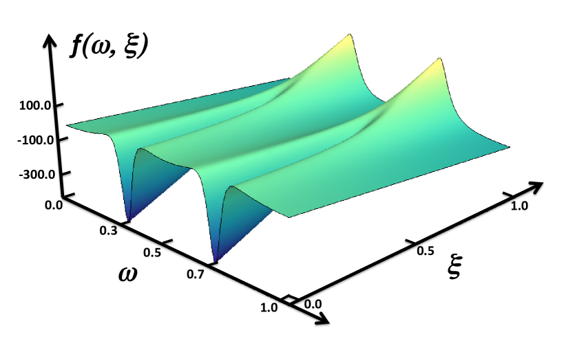
Figure 1: (Color online) Graphical illustration of the subtraction procedure. The explanation is in the text.

The subtraction procedure can also be illustrated graphically, as in Fig. 1, by plotting a “model function” $f(\omega,\xi)$ in terms of its two arguments, which we assume to be scaled dimensionless parameters $\omega,\xi\in(0,1)$. For $\xi=1$, we plot the na$\ddot{\mbox{\i}}$vely regularized model function

$$f(\omega,\xi=1)=\left|\frac{1}{\omega_{0}-\omega+\mathrm{i}\epsilon}\right|^{2}+\left|\frac{1}{\omega_{1}-\omega+\mathrm{i}\epsilon}\right|^{2}-\frac{2\pi}{\epsilon}\,,$$ (14)

illustrating the na$\ddot{\mbox{\i}}$ve regularization. This function has two maxima near $\omega_{0}=0.3$ and $\omega_{1}=1-\omega_{0}$ which approximate the peaks in the two-photon spectrum under the presence of a virtual resonant state which is displaced from the initial state of the two-photon process by the energy $\omega_{0}=0.3$. We use a numerically small regulator value $\epsilon=0.01$ in accordance with the basic assumptions on which our derivation is based; if $\epsilon$ were large, then, e.g., argument regarding the “trapping” of the electron in the intermediate states as given in Sec. IV would break down. The term $-2\pi/\epsilon$ is subtracted in order to ensure that the function $f(\omega,\xi=1)$ has the same integral over $\omega\in(0,1)$ as the QED regularized expression

$$f(\omega,\xi=0)={\rm Re}\left\{\frac{1}{(\omega_{0}-\omega+\mathrm{i}\epsilon)^{2}}+\frac{1}{(\omega_{1}-\omega+\mathrm{i}\epsilon)^{2}}\right\}\,,$$ (15)

which has two minima near $\omega_{0}$ and $\omega_{1}$ and illustrates the $\mathrm{i}\epsilon$ prescription. The interpolation

$$f(\omega,\xi)=\xi\,\,f(\omega,1)+(1-\xi)\,\,f(\omega,0)$$ (16)

illustrates that in view of the negative tilt of $f(\omega,\xi)$ along the $\xi$ axis, the integral $\int_{0}^{1}\mathrm{d}\omega\,f(\omega,\xi)$, i.e., the “decay rate,” is independent of $\xi$ and thus the same in both regularizations ($\xi=0$ versus $\xi=1$).

References

- (1) M. Göppert-Mayer, Ann. Phys. (Leipzig) 401, 273 (1931).
- (2) V. Florescu, Phys. Rev. A 30, 2441 (1984).
- (3) J. H. Tung, X. M. Ye, G. J. Salamo, and F. T. Chan, Phys. Rev. A 30, 1175 (1984).
- (4) J. D. Cresser, A. Z. Tang, G. J. Salamo, and F. T. Chan, Phys. Rev. A 33, 1677 (1986).
- (5) V. Florescu, S. Patrascu, and O. Stoican, Phys. Rev. A 36, 2155 (1987).
- (6) V. Florescu, I. Schneider, and I. N. Mihailescu, Phys. Rev. A 38, 2189 (1988).
- (7) J. Chluba and R. A. Sunyaev, e-print 0705.3033 [astro-ph].
- (8) H. A. Bethe and E. E. Salpeter, Quantum Mechanics of One- and Two-Electron Atoms (Springer, Berlin, 1957).
- (9) U. D. Jentschura, J. Phys. A 41, 155307 (2008).
- (10) U. D. Jentschura, J. Phys. A 40, F223 (2007).
- (11) U. D. Jentschura and A. Surzhykov, Phys. Rev. A 77, 042507 (2008).
- (12) R. Barbieri and J. Sucher, Nucl. Phys. B 134, 155 (1978).
- (13) V. I. Ritus, Nucl. Phys. B 44, 236 (1972).
- (14) U. D. Jentschura, G. Soff, and P. J. Mohr, Phys. Rev. A 56, 1739 (1997).
- (15) A. R. Edmonds, Angular Momentum in Quantum Mechanics (Princeton University Press, Princeton, New Jersey, 1957).
- (16) D. A. Varshalovich, A. N. Moskalev, and V. K. Khersonskii, Quantum Theory of Angular Momentum (World Scientific, Singapore, 1988).
- (17) R. de la Madrid and M. Gadella, Am. J. Phys. 70, 626 (2002).
- (18) H. A. Bethe, Phys. Rev. 72, 339 (1947).
- (19) P. J. Mohr, Ann. Phys. (N.Y.) 88, 26 (1974).
- (20) P. J. Mohr, Ann. Phys. (N.Y.) 88, 52 (1974).
- (21) U. D. Jentschura and C. H. Keitel, Ann. Phys. (N.Y.) 310, 1 (2004).
- (22) M. Baranger, Phys. Rev. 84, 866 (1951), [Erratum Phys. Rev. 85, 1064 (1952)].
- (23) M. Baranger, H. A. Bethe, and R. P. Feynman, Phys. Rev. 92, 482 (1953).
- (24) K. Pachucki, J. Phys. B 31, 5123 (1998).
- (25) V. N. Baier, V. M. Katkov, and V. M. Strakhovenko, Electromagnetic Processes At High Energies in Oriented Single Crystals (World Scientific, Singapore, 1998).