Quark number Susceptibility and Phase Transition in hQCD Models

Abstract:

We study the quark number susceptibility, an indicator of QCD phase transition, in the hard wall and soft wall models of hQCD. We find that the susceptibilities in both models are the same, jumping up at the deconfinement phase transition temperature. We also find that the diffusion constant in the soft wall model is enhanced compared to the one in the hard wall model.

1 Introduction

There has been much interest in applying the idea of AdS/CFT[1] in strong interaction. After initial set up for N=4 SYM theory, confining theories were treated with IR cut off at the AdS space[2] and quark flavors [3] were introduced by adding extra probe branes. More phenomenological models were also suggested to construct a holographic model dual to QCD [4, 5, 6, 7]. The finite temperature version of such model were suggested in [8, 9, 10]. For the purose of the Regge trajectory, quadratic dilaton background was introduced Ref. [11] whose role is to prevent string going into the deep inside the IR region of AdS space by a potential barrier and as a consequence the particle spectrum rise more slowly compared with hard-wall cutoff. Remarkably such a dilaton-induced potential gives exactly the linear trajectory of the meson spectrum. In [12], it was argued that such a dilatonic potential could be motivated by instanton effects.

The quark number susceptibility $\chi_{q}$, which measures the response of QCD to a change in the chemical potential, was proposed as a probe of the QCD chiral/deconfinement phase transition at zero chemical potential [13, 14]. It is one of the thermodynamic observables that can reveal a character of chiral phase transition. The lattice QCD calculation  [13] showed the enhancement of the susceptibility around $T_{c}$ by a factor 4 or 5. Since then, various model studies [15, 16, 17] and lattice simulations  [18, 19, 20, 21, 22, 23] have been performed to calculate the susceptibility.

In this work, we calculate the quark number susceptibility and study QCD chiral/deconfinement phase transition in holographic QCD models [6, 7, 9, 11]. In the models adopted in the present work, we implicitly assume that chiral symmetry restoration and deconfinement take place at the same critical temperature $T_{c}$.

In a gravity dual of QCD-like model, the confinement to de-confinement phase transition is described by the Hawking-Page transition (HPT). At low temperature, thermal AdS dominates the partition function, while at high temperature, AdS-black hole geometry dominates. This was first discovered in the finite volume boundary case in [8], and more recently it is shown in [25] that the same phenomena happen also for infinite boundary volume, if there is a finite scale along the fifth direction. In our work, both hard wall [6] and soft wall [11] models are considered, where we have a definite IR scale, so that we are dealing with theories with deconfinement phase transition.

In the presence of the AdS black hole, the most physical boundary condition is the infalling one. In the hard wall model [6, 7] that the infalling boundary condition in the zero frequency and momentum limit can be understood as a conformally invariant Dirichlet condition. In the the soft wall model [11], we calculate the quark number susceptibility and find that it is the same with the one obtained in the hard wall model, while diffusion constant of the soft wall model is enhanced compared to the hard wall model.

The rest of the paper goes as follows. In section 2, we briefly summarize the holographic QCD models adopted in the present work and discuss the chiral symmetry restoration in the models. In section 3, we calculate the quark number susceptibility in the AdS black hole background, adopting the infalling boundary condition, in the hard wall and soft wall models. Section 4 gives summary. In Appendix A, we re-evaluate the susceptibility with the Dirichlet boundary condition followed by the implication of the Hawking-Page transition [25]

2 Holographic QCD and chiral symmetry at finite temperature

2.1 Chiral symmetry in Hard wall model:

The action of the holographic QCD model suggested in [6, 7, 9] is given by

$${\rm S}_{\rm I}=\int d^{4}xdz\sqrt{g}{\cal L}_{5}\,,$$

$$\,\,\,\,{\cal L}_{5}={\rm Tr}\biggl{[}-\frac{1}{4g_{5}^{2}}(L_{MN}L^{MN}+R_{MN}R^{MN})+|D_{M}\Phi|^{2}-M_{\Phi}^{2}|\Phi|^{2}\biggr{]}\,,$$ (1)

where $D_{M}\Phi=\partial_{M}\Phi-iL_{M}\Phi+i\Phi R_{M}$ and $L_{M}=L_{M}^{a}\tau^{a}/2$ with $\tau^{a}$ being the Pauli matrix. The scalar field is defined by $\Phi=S{\mbox{e}}^{i\pi^{a}\tau^{a}}$ and $<S>\equiv\frac{1}{2}v(z)$, where $S$ is a real scalar and $\pi$ is a pseudoscalar. Under ${\rm SU(2)}_{V}$, $S$ and $\pi$ transform as singlet and triplet. In this model, the 5D AdS space is compactified such that $0<z\leq z_{m}$.

As in  [9], we work on the 5D AdS-Schwarzchild background, which is known to describe the physics of the finite temperature in dual 4D field theory side,

$$ds_{5}^{2}=\frac{1}{z^{2}}\biggl{(}f(z)dt^{2}-(dx^{i})^{2}-\frac{1}{f(z)}dz^{2}\biggr{)},~{}~{}f(z)=1-\frac{z^{4}}{z_{T}^{4}},$$ (2)

where $i=1,2,3.$ Here the temperature is defined by $T=1/(\pi z_{T})$, and the Hawking-Page transition [25] occurs at $T_{c}=2^{1/4}/(\pi z_{m})$. For the temperature lower than $T_{c}$, thermal AdS dominates, and it is hard to find temperature dependence in low temperature regime, which is actually consistent with the earlier work on large N gauge theory [24].

The equation of motion for $v(z)$ in the black hole background is

$$\biggl{[}\partial_{z}^{2}-\frac{4-f}{zf}\partial_{z}+\frac{3}{z^{2}f}\biggr{]}v(z)=0\,,$$ (3)

and the solution is given by [9]

$$v(z)=M_{q}z~{}{}_{2}F_{1}(\frac{1}{4},\frac{1}{4},\frac{1}{2},\frac{z^{4}}{z_{T}^{4}})+\Sigma_{q}z^{3}~{}{}_{2}F_{1}(\frac{3}{4},\frac{3}{4},\frac{3}{2},\frac{z^{4}}{z_{T}^{4}}).$$ (4)

Here $M_{q}$ and $\Sigma_{q}$ are identified with the current quark mass and the chiral condensate respectively. Note that at $z=z_{T}$, both terms in $v(z)$ diverges logarithmically. This requires us to set both of them to be zero,

$$M_{q}=0,\quad\quad\Sigma_{q}=0.$$ (5)

The latter condition means that the chiral symmetry is restored, and deconfinement and the chiral phase transition take place at the same temperature. It is interesting to observe that the mass term is also forbidden in this phase. This is consistent with the fact that the chiral symmetry forbids fermion mass term. In reality the chiral symmetry is partially broken in low temperature and also partially restored in the high temperature due to the current quark mass. In this sense, the hard wall model respects the chiral symmetry more than the reality.

2.2 Chiral symmetry in Soft wall model

In [11], dilaton background was introduced for the Regge behavior of the spectrum.

$${\rm S}_{\rm II}=\int d^{4}xdz{\mbox{e}}^{-\Phi}{\cal L}_{5}\,,$$ (6)

where $\Phi=cz^{2}$. Here the role of the hard-wall IR cutoff $z_{m}$ is replaced by a dilaton-induced potential. The equation of motion for $v(z)$ is given by

$$\biggl{[}\partial_{z}^{2}-(2cz+\frac{4-f}{zf})\partial_{z}+\frac{3}{z^{2}f}\biggr{]}v(z)=0\,.$$ (7)

At zero temperature [11], where $f=1$, one of the two linearly independent solutions of Eq. (7) diverges as $z\rightarrow\infty$, and so we have to discard this solution. Then chiral condensate is simply proportional to $M_{q}$ [11]. Now we consider a finite temperature case. Near $z_{T}$, $c$ dependent term in Eq. (7) is negligible and there is no difference between hard and soft wall model near the horizon. So we can draw the same conclusion of the complete chiral symmetry restoration.

3 Quark number susceptibility

In this section, we calculate the quark number susceptibility at high temperature in deconfinement phase. The relevant background is the AdS black hole,

$$ds^{2}=\frac{(\pi T)^{2}}{u}\bigg{(}f(u)dt^{2}-(dx^{i})^{2}\bigg{)}-\frac{1}{4u^{2}f(u)}du^{2}$$ (8)

where u=$(z/z_{T})^{2}$, f(u) = 1-$u^{2}$ and T = $1/\pi z_{T}$.

The quark number susceptibility was proposed as a probe of the QCD chiral phase transition at zero chemical potential [13, 14].

$$\chi_{q}=\frac{\partial n_{q}}{\partial\mu_{q}}.$$ (9)

The quark number susceptibility can be written in terms of the retarded Green’s function. Here we follow the procedure given in [15]. First we write

$$\chi_{q}(T,\mu)=\beta\int d^{3}xG_{00}(0,x),$$ (10)

where the vector correlator at finite temperature is defined by

$$G^{\mu\nu}(p;T)\delta_{ab}=\int_{0}^{1/T}d\tau\int d^{3}\vec{x}e^{-ip\cdot{x}}\left\langle J_{a}^{\mu}(\tau,\vec{x})J_{b}^{\nu}(0,\vec{0})\right\rangle_{\beta}\,.$$ (11)

After the Fourier transformation, we obtain

$$\chi_{q}(T,\mu)=\lim_{k\rightarrow 0}\int^{\infty}_{-\infty}\frac{d\omega}{2\pi}G_{00}(\omega,k)$$ (12)

By the fluctuation-dissipation theorem, we have

$$G_{00}(\omega,k)=-\frac{2}{1-{\mathrm{e}}^{-w/T}}{\mathrm{Im}}G^{R}_{00}(\omega,k)$$ (13)

where $G^{R}_{00}(\omega,k)$ is retarded Greens function of $j_{\mu},j_{\nu}$. Then we arrive at

$$\chi_{q}(T,\mu)=-\lim_{k\rightarrow 0}\int^{\infty}_{-\infty}\frac{d\omega}{2\pi}\frac{2}{1-{\mathrm{e}}^{-w/T}}{\mathrm{Im}}G^{R}_{00}(\omega,k)$$ (14)

The $\mathrm{Im}G_{00}^{R}(\omega,k)$ is related to the real part of Green’s function through the Kramers-Kronig dispersion relations,

$$\mathrm{Re}G_{00}^{R}(\omega,k)=\mathcal{P}\int^{\infty}_{-\infty}\frac{d\omega^{\prime}}{\pi}\frac{\mathrm{Im}G^{R}_{00}(\omega,k)}{w^{\prime}-w}\,.$$ (15)

One can easily see that $\chi_{q}$ is written in the following form,

$$\chi_{q}(T,\mu_{q})=-\lim_{k\rightarrow 0}\mathrm{Re}G_{00}^{R}(0,k)\,.$$ (16)

What is the physics we want to see? The lattice QCD calculations  [13, 18, 19, 22] showed the enhancement of $\chi_{q}$ around $T_{c}$:

$$R_{\chi}\equiv\frac{\chi_{q}(T_{c}+\epsilon)}{\chi_{q}(T_{c}-\epsilon)}=4\sim 5\,.$$ (17)

The enhancement in $R_{\chi}$ may be understood roughly as follows  [14]. At low temperature, in confined phase $\chi_{q}$ will pick up the Boltzmann factor ${\mbox{e}}^{-M_{N}/T}$, where $M_{N}$ is a typical hadron mass scale $\sim 1~{}{\rm GeV}$, while at high temperature the factor will be given in terms of a quark mass ${\mbox{e}}^{-M_{q}/T}$, and therefore there could be some enhancement. In Ref. [15], it is shown that the enhancement in $\chi_{q}$ may be due to the vanishing or a sudden decrease of the interactions between quarks in the vector channel.

In the holographic QCD models, due to the HPT [25], the quark number susceptibility is described by the AdS black hole background at high temperature and by the thermal AdS at low temperature. We will patch them together. We calculate the susceptibility both in the hard wall model  and in the soft wall model and describe how it changes under the phase transition.

3.1 Hard wall model

The temperature dependence of confinement phase can not be extracted from the AdS black hole due to the Hawking-Page transition. That is, thermal AdS replaces the AdS black hole at low temperature. Therefore we need to consider two phase separately.

3.1.1 Confined phase

We take the thermal AdS with hard wall at $z=z_{m}$ as the dual gravity background. From the quadratic part of the 5D action Eq. (1), we obtain the equation of motion for the time component vector meson

$$\biggl{[}\partial_{z}^{2}-\frac{1}{z}\partial_{z}+\vec{q}^{2}\biggr{]}V_{0}(z,\vec{q})=0.\,$$ (18)

Note that in the above equation, the $q_{0}\to 0$ limit is already taken, following the definition given in Eq. (16). With a finite $q_{0}$ the equation will couple to other components. We solve Eq. (18) in a limit where ${\vec{q}}\to 0$. The solution is $V_{0}=a_{1}-a_{2}z^{2}\,.$ According to the AdS/CFT dictionary, $V_{0}$ is dual to the number density $j^{0}(x)$ in boundary, hence we can identify $a_{1}$ as the chemical potential $\mu$ and the $a_{2}$ as the charge density $Q$. Therefore

$$V_{0}=\mu-Q(z/z_{m})^{2}\,.$$ (19)

Then the quark number susceptibility is given by

$$\chi_{q}(T) = -\left[\frac{1}{g_{5}^{2}}\frac{\partial_{z}V_{0}}{z}\right]_{z=0}=\frac{2Q/z_{m}^{2}}{g_{5}^{2}}\,.$$ (20)

For the black hole background, we have to request $V_{0}=0$ at the horizon for the regularity of the vector field, making $\mu$ proportional to $Q$. However, for the thermal AdS there is no such requirement to be imposed. Therefore, even when a charge is zero, one can still have a finite chemical potential in confining case. However, in the limit where the chemical potential is zero, the charge density must be zero, otherwise we would need work to bring a particle into the system, requesting a finite chemical potential. That is, in the limit of zero chemical potential we should have zero charge and hence

$$\chi_{q}=0,$$ (21)

in the confined phase.

3.1.2 Deconfined phase

Here we calculate the quark number susceptibility in deconfined phase on the metric (8). Note that the role of the IR cutoff $z_{m}$ is none in the deconfined phase. The action of the gauge field, which is dual to the 4D quark current $j_{\mu}=\bar{q}(t,\vec{x})\gamma_{\mu}q(t,\bar{x})$, is

$$S=-\int d^{5}x\sqrt{g}\frac{1}{4g_{5}^{2}}F_{MN}F^{MN}\,,$$ (22)

where $1/g_{5}^{2}=N_{c}N_{f}/(2\pi)^{2}$ coming from the D3/D7 model [36]. In the presence of the AdS black hole, the most natural boundary condition is the infalling boundary condition since the black hole can only absorb classically. For the static case, we may consider the Dirichlet and Neumann boundary conditions. To impose the infalling boundary condition, we solve the problem at small but non-zero frequency and momentum and then take them to be zero. This is the problem considered in the literature on hydrodynamics [28]. Notice that in terms of the re-scaled coordinate $u=(z/z_{T})^{2}$, the momentum $k=(\omega,0,0,q)$ enters in the action only in the combination of $\textswab{w}=\frac{\omega}{2\pi T},\quad\textswab{q}=\frac{q}{2\pi T}$. The relevant equations of motion for the vector fields in the $A_{u}=0$ gauge are

$$\textswab{w}A_{0}^{\prime}+\textswab{q}f\,A_{3}^{\prime}=0\rule[-14.45377pt]{0.0pt}{14.45377pt}\,,\quad A_{0}^{\prime\prime}-\frac{1}{uf}\left(\textswab{q}^{2}A_{0}+\textswab{w}\textswab{q}A_{3}\right)=0\,,\rule[-14.45377pt]{0.0pt}{14.45377pt}$$ (23)

$$A_{3}^{\prime\prime}+{f^{\prime}\over f}A_{3}^{\prime}+\frac{1}{uf^{2}}\left(\textswab{w}^{2}A_{3}+\textswab{w}\textswab{q}A_{0}\right)=0\,,\rule[-14.45377pt]{0.0pt}{14.45377pt}$$ (24)

where ^′ means $\partial_{u}$. Out of the coupled equations we can eliminate $A_{3}$ to get a second order differential equation for $A^{\prime}_{0}:=\Psi$.

$$\Psi^{\prime\prime}+\frac{(uf)^{\prime}}{uf}\Psi^{\prime}+{\textswab{w}^{2}-\textswab{q}^{2}f(u)\over uf^{2}}\Psi=0\,,$$ (25)

After taking out the near horizon behavior $\sim(1-u)^{-i\textswab{w}/2}$ of infalling wave, one can extract the small frequency behavior of the residual part using Mathematica. The result is

$$\Psi=(1-u)^{-i\textswab{w}/2}\cdot\frac{\textswab{q}^{2}A_{0}^{0}+\textswab{w}\textswab{q}A_{3}^{0}}{(i\textswab{w}-\textswab{q}^{2})}\Bigl{(}1+\frac{i\textswab{w}}{2}\ln\frac{2u^{2}}{1+u}-\textswab{q}^{2}\ln\frac{2u}{1+u}+\cdots\Bigr{)},$$ (26)

where $A_{\mu}^{0}$ is the boundary value of $A_{\mu}$. With the prescription for the retarded Green function

$$G_{\mu\nu}^{R}(k)=\frac{\delta^{2}S}{\delta A_{\mu}^{0}(-k)\delta A_{\nu}^{0}(k)},$$ (27)

with

$$S=\frac{\pi^{2}T^{2}}{g_{5}^{2}}\int d^{4}k\Bigl{[}\Psi(-k)\Psi(k)+\cdots\Bigr{]}_{u=0}.$$ (28)

one can get the retarded Green function

$$\begin{split}G^{R}_{\mu\nu}(\omega,\bm{q})&=-i\!\int\!d^{4}x\,e^{-iq\cdot x}\,\theta(t)\langle[J_{\mu}(x),\,J_{\nu}(0)]\rangle\end{split}$$ (29)

in small frequency;

$$G^{R}_{00} = \frac{2\pi^{2}T^{2}}{g_{5}^{2}}{\textswab{q}^{2}\;\over(i\textswab{w}-\textswab{q}^{2}+i\textswab{w}^{2}\ln 2/2)}\Bigl{(}1+\ln 2\,\Bigl{(}\frac{i}{2}\textswab{w}-\textswab{q}^{2}\Bigr{)}\Bigr{)}$$ (30)

Finally, by using eq. (16), we get the susceptibility

$$\chi_{q}=\frac{2\pi^{2}T^{2}}{g_{5}^{2}}=\frac{N_{c}N_{f}}{2}T^{2}\,.$$ (31)

$\chi_{q}/T^{2}$ is a constant which is consistent with high temperature behavior of lattice result  [13, 18, 19, 20, 21, 22, 23]. Our results show that $\chi_{q}(T)/T^{2}$ jumps from zero, corresponding to the thermal AdS phase, to a constant, AdS black hole phase, with increasing the temperature. We plot $\chi_{q}$ as a function of temperature.

We close this section with an interesting observation. If we impose the Dirichlet condition at the horizon, $V_{0}(z_{T})=h$, we get

$$\chi_{q}(T)=\frac{2\pi^{2}}{g_{5}^{2}}(1-h)T^{2}\,,$$ (32)

Notice that for the conformally invariant choice $h=0$, Dirichlet condition gives the identical result to the infalling BC obtained above.

3.2 Soft wall model

Now we consider the soft wall model. The action is given by

$$S=-\int d^{5}x\sqrt{g}\mathrm{e}^{-\Phi}\frac{1}{4g_{5}^{2}}F_{MN}F^{MN},\quad\Phi=\frac{c}{(\pi T)^{2}}u.$$ (33)

In this model, there is also the Hawking-Page transition [25]. The equation of motion for $V_{0}$ in the static-low momentum limit reads

$$\partial_{z}(\frac{1}{z}{\mbox{e}}^{-cz^{2}}\partial_{z}V_{0})=0\,,$$ (34)

whose solution is given by

$$V_{0} = a{\mbox{e}}^{cz^{2}}+b\,,$$ (35)

$$\simeq c_{1}+c_{2}z^{2}\,,z\rightarrow 0\,.$$

Then, following the same argument given in (3.1.1), we conclude that the quark number susceptibility is also zero in the soft wall model at low temperature.

Now we consider high temperature phase. The relevant equations of motion are

$$A_{t}: A_{t}^{\prime\prime}-\frac{c}{(\pi T)^{2}}A_{t}^{\prime}-\frac{1}{uf(u)}(\textswab{q}^{2}A_{t}+\textswab{q}\textswab{w}A_{z})=0$$ (36)

$$A_{\alpha}: A^{\prime\prime}_{\alpha}+(\frac{-c}{(\pi T)2}+\frac{f^{\prime}(u)}{f(u)})A^{\prime}_{\alpha}+\frac{1}{uf(u)}(\frac{\textswab{w}^{2}}{f(u)}-\textswab{q}^{2})A_{\alpha}=0$$ (37)

$$A_{z}: A^{\prime\prime}_{z}+(\frac{-c}{(\pi T)2}+\frac{f^{\prime}(u)}{f(u)})A^{\prime}_{z}+\frac{1}{uf(u)^{2}}(\textswab{w}\textswab{q}A_{t}-\textswab{w}^{2}A_{z})=0$$ (38)

$$A_{u}: \textswab{w}A^{\prime}_{t}+\textswab{q}f(u)A^{\prime}_{z}=0$$ (39)

From the eq.(36), we can express $A_{z}$ in terms of $A_{t}$

$$A_{z}=\frac{uf(u)}{\textswab{q}\textswab{w}}\left(A^{\prime\prime}_{t}-\frac{c}{(\pi T)^{2}}A^{\prime}_{t}-\frac{\textswab{q}^{2}}{uf(u)}A_{t}\right)\,.$$ (40)

Inserting it to eq.(39), we obtain

$$A^{\prime\prime\prime}+\Big{(}\frac{1-3u^{2}}{uf}-c_{T}\Big{)}A^{\prime\prime}+\frac{1}{uf^{2}}\Big{(}\textswab{w}^{2}-f(c_{T}(1-3u^{2})+\textswab{q}^{2})\Big{)}A^{\prime}=0$$ (41)

where $c_{T}=c/(\pi T)^{2}$. Imposing the infalling boundary condition at the horizon, we take $A^{\prime}_{t}=(1-u)^{-i\mathbf{w}/2}$ F(u) to obtain

$$F^{\prime\prime}+(-\frac{c}{(\pi T)^{2}}+\frac{1-3u^{2}}{uf(u)}+i\frac{\mathbf{w}}{1-u})F^{\prime}$$

$$+\bigg{(}-\frac{c}{(\pi T)^{2}}(\frac{1-3u^{2}}{uf(u)})+\textswab{w}\Big{(}\frac{i(1+2u)}{2uf(u)}-\frac{c}{(\pi T)^{2}}\frac{i(1+u)}{2f(u)}\Big{)}$$

$$+\textswab{w}^{2}\frac{4-u(1+u)^{2}}{4uf(u)^{2}}-\frac{\textswab{q}^{2}}{uf(u)}\bigg{)}F=0.$$ (42)

In the long-wavelength, low frequency limit, F(u) can be expanded as series in $\textswab{w},\textswab{q}^{2}$,

$$F(u)=F_{0}+\textswab{w}F_{1}(u)+\textswab{q}^{2}G_{1}+\cdots$$ (43)

After some algebra, we obtain first a few terms

$$F_{0} = B$$ (44)

$$F_{1} = \frac{iB\mathrm{e}^{-c_{T}}}{12}\bigg{(}2(\mathrm{e}^{c_{T}}-\mathrm{e}^{c_{T}u})+(-12+5c_{T})\mathrm{e}^{c_{T}(1+u)}\Big{(}Ei(-c_{T})-Ei(-c_{T}u)\Big{)}\rangle$$ (45)

$$-2\mathrm{e}^{c_{T}(2+u)}(-3+c_{T})\{Ei(-2c_{T})-Ei(-c_{T}(1+u))\}\bigg{)}$$

$$G_{1} = B\mathrm{e}^{c_{T}u}\bigg{(}Ei(-c_{T})-Ei(-c_{T}u)+\mathrm{e}^{c_{T}}\Big{(}Ei(-c_{T}(1+u))-Ei(-2c_{T})\Big{)}\bigg{)}\,,$$ (46)

where Ei(x) is defined as the principal value of $Ei(z)=-\int_{-z}^{\infty}\left.e^{-t}\right/t\,dt$. The integration constants of $F_{1}$, $G_{1}$ are chosen by the regularity condition at u=1. B is determined from the boundary values of $A_{t}$ and $A_{z}$ at u=0.

$$B=\frac{\textswab{q}^{2}A_{t}^{0}+\textswab{q}\textswab{w}A_{z}^{0}}{i\textswab{w}(1-\frac{5}{12}c_{T})-\textswab{q}^{2}}.$$ (47)

From these results, $A_{t}^{\prime}(u)$ is

$$A^{\prime}_{t}(u)=(1-u)^{-i\mathbf{w}/2}\frac{\textswab{q}^{2}A_{t}^{0}+\textswab{q}\textswab{w}A_{z}^{0}}{i\textswab{w}(1-\frac{5}{12}c_{T})-\textswab{q}^{2}}\bigg{(}1+\textswab{q}^{2}X_{\textswab{q}^{2}}+i\frac{\textswab{w}}{12}Y_{\textswab{w}}\bigg{)}\,,$$ (48)

where $X_{\textswab{q}^{2}},Y_{\textswab{w}}$ are

$$X_{\textswab{q}^{2}} = \mathrm{e}^{c_{T}u}\bigg{(}Ei(-c_{T})-Ei(-c_{T}u)-\mathrm{e}^{c_{T}}\Big{(}Ei(-2c_{T})-Ei(-c_{T}(1+u))\Big{)}\bigg{)}$$

$$Y_{\textswab{w}} = \mathrm{e}^{c_{T}u}\bigg{(}2\mathrm{e}^{-c_{T}u}-2\mathrm{e}^{-c_{T}}+(-12+5c_{T})\Big{(}Ei(-c_{T})-Ei(-c_{T}u)\Big{)}$$ (49)

$$-2\mathrm{e}^{c_{T}}(-3+c_{T})\Big{(}Ei(-2c_{T})-Ei(-c_{T}(1+u))\Big{)}\bigg{)}\,.$$

The real part of the retarded Green’s function

$$\mathrm{Re}G_{00}^{R}(k)=-\frac{2\pi^{2}T^{2}}{g_{5}^{2}}\frac{q^{2}}{P^{2}w^{2}+\bar{D}^{2}q^{4}}\left(\bar{D}^{2}q^{2}+\bar{D}^{4}q^{4}X_{\textswab{q}^{2}}(\epsilon)-\frac{w^{2}}{12}\bar{D}^{2}PY_{\textswab{w}}(\epsilon)\right)\,,$$ (50)

where $\bar{D}=1/2\pi T$ and $P=1-5c/12\pi^{2}T^{2}$. Note that the Green function has diffusion pole, and the diffusion constant is

$$D=\frac{1}{2\pi T}\frac{1}{1-\frac{5c}{12\pi^{2}T^{2}}}.$$ (51)

Notice that it is dressed by the factor $1/P$ due to the effect of the soft wall. One can easily check the positivity of the diffusion constant in the relevant temperature regime

$$P=1-0.17\frac{T_{c}^{2}}{T^{2}}>0,\quad{\mathrm{if}~{}T>T_{c}}$$ (52)

where $T_{c}=1/\pi^{2}{z_{c}}^{2}$, and we used $c{z_{c}}^{2}=0.42$ [25].

The quark number susceptibility is obtained with eq.(16) and we get

$$\chi_{q}=\frac{2\pi^{2}T^{2}}{g_{5}^{2}}\,,$$ (53)

which is the same with the result of the hard wall model.

Putting together the results at low and high temperatures, we arrive at the following conclusion. $\chi_{q}$ is zero up to the phase transition temperature, and it jumps to a finite value given in Eq. (53), which implies a first order phase transition between low- and high-temperature phases. The sharp transition might be the large $N_{c}$ artifact.

In hard wall case we observed that the infalling and (a specially chosen) Dirichlet boundary conditions give the same results. One may wonder if one can arrive at the same conclusion in the soft wall model. In Appendix we dig into this question to observe that those two boundary conditions lead to different susceptibilities.

4 Summary

We first discussed the chiral symmetry restoration in AdS/QCD models. The AdS/QCD models respect the chiral symmetry more rigidly than the reality in the sense that, in chiral symmetry restored phase, both of the chiral condensate and the mass of the quarks are zero.

Then, we calculated the quark number susceptibility in both hard wall and soft wall models. At low temperature, in confined phase, we showed that $\chi_{q}$, which is defined in the limit of zero chemical potential, is zero. With the infalling boundary condition, we could uniquely determine the overall normalization of the susceptibility, unlike the Dirichlet boundary condition. We found that the susceptibilities in both models are the same with the infalling boundary condition, and $\chi_{q}\sim T^{2}$ at high temperature, which is consistent with high-temperature lattice QCD observations [18, 19, 20, 21, 22, 23].

In Appendix A, we considered Dirichlet boundary condition in the soft wall model. With the HPT, we predicted the temperature dependence of $\chi_{q}$ at high temperature apart from the overall normalization that is fixed by an IR boundary condition. Our result with the HPT exhibits a similar behavior observed in model studies [15, 16, 17] and lattice simulations  [18, 19, 20, 21, 22, 23].

Regardless of the IR boundary conditions, our results in both models predicted a sharp jump in the quark number susceptibility, which is an unavoidable aspect of the HPT and could be smoothed out by including large $N_{c}$ corrections.

Finally, we discuss a limitation of our approach in the light of the QCD phase transition. The nature of the QCD transition depends on the number of quark flavors and the quark mass: for pure SU(3) gauge theory, it is a first order, for two massless quarks, it is a second order, for two quarks with finite masses, it is a cross over, for three degenerate massless quarks, it is a first order, etc. Unlike the Polyakov loop or chiral condensate, the quark number susceptibility is not an order parameter, and so in the present study we are not able to determine the order of the QCD phase transition. The susceptibility could serve, at best, as an indicator of the transition.

Appendix A Dirichlet boundary condition in soft wall model

Here we give analysis with Dirichlet boundary conditions in high temperature. The equation of motion for $V_{0}$ in the static, zero momentum limit is the same as eq.(34) and the solution is still given by $V_{0}=a{\mbox{e}}^{cz^{2}}+b$. However, with the Dirichlet boundary conditions $V_{0}(0)=1,\;\;V_{0}(z_{T})=0$, the result is given by

$$\chi_{q}(T)=\frac{2c}{g_{5}^{2}}\frac{1}{{\mbox{e}}^{{\tilde{T}}_{c}^{2}/T^{2}}-1}$$ (54)

We note here that $\chi_{q}({T}_{0})\approx 1.2{\tilde{T}}_{c}^{2}$, where ${T}_{0}=\sqrt{c}/\pi$ is the temperature scale generated by $c$.

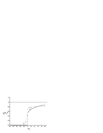
Figure 1: (a) $\chi_{q}$ in hQCD with the innfalling boundary condition discussed in section 3. (b) $\chi_{q}$ in the soft wall model with the Dirichlet boundary condition. The circles are for the (quenched) lattice QCD results as shown in Ref. [15, 19], and the triangles are for full lattice QCD in [20].

Appendix B parameters of the soft-wall models

The masses of the vector mesons are given by $m_{n}^{2}=4c(n+1)$. If we use $m_{1}=770~{}{\rm MeV}$ and $m_{2}=1450~{}{\rm MeV}$ to calculate the slope of the Regge trajectory, then we obtain $\sqrt{c}\simeq 614~{}{\rm MeV}$ and so end up with the reasonable value of the transition temperature $T_{c}\simeq 195~{}{\rm MeV}$. The value of $T_{c}$ was determined in Ref. [31], $T_{c}=210~{}{\rm MeV}$, and more recently the relation between $T_{c}$ and $z_{m}$ ($\sqrt{c}$) is obtained through Hawking-Page analysis in the holographic models used in this work, where $T_{c}\approx 191~{}{\rm MeV}$ [25]. We note here that in [32], the value of $\sqrt{c}$ was determined to be $\sim 671~{}{\rm MeV}$. Finally, we relate $c$ with the QCD string tension $\sigma$. The masses of vector towers are given, in terms of $\sigma$, by $m_{n}^{2}=2\pi\sigma n$. From this and $m_{n}^{2}=4c(n+1)$, we get $c=\frac{\pi}{2}\sigma,$ so that the dilaton factor becomes ${\mbox{e}}^{-\frac{\pi}{2}\sigma z^{2}}$. Note that the relation between $c$ and string tension was also observed in Ref. [34].

Acknowledgments
We thank Seyong Kim for useful information on lattice QCD and Ho-Ung Yee for helpful discussions. The work of SJS was supported by the SRC Program of the KOSEF through the Center for Quantum Space-time(CQUeST) of Sogang University with grant number R11 - 2005 - 021 and also by KOSEF Grant R01-2007-000-10214-0. The work of KJ is supported in part by the Seoul Fellowship.

References

-
[1]
J. Maldacena, Adv. Theor. Math. Phys. 2 (1998) 231;
S.S. Gubser, I.R. Klebanov and A.M. Polyakov, Phys. Lett. B428 (1998) 105;
E. Witten, Adv. Theor. Math, Phys. 2 (1998) 253. - [2] J. Polchinski and M. J. Strassler, Phys. Rev. Lett. 88 (2002) 031601; hep-th/0109174.
- [3] A. Karch and E. Katz, JHEP 0206, 043 (2002) [arXiv:hep-th/0205236].
- [4] S. J. Brodsky and G. F. de Teramond, Phys. Rev. Lett. 96, 201601 (2006) [hep-ph/0602252].
- [5] T. Sakai and S. Sugimoto, Prog. Theor. Phys. 113, 843 (2005)[hep-th/0412141]; 114, 1083 (2006) [hep-th/0507073]
- [6] J. Erlich, E. Katz, D. T. Son and M. A. Stephanov, Phys. Rev. Lett. 95, 261602 (2005) [hep-ph/0501128].
- [7] L. Da Rold and A. Pomarol, Nucl.Phys. B721, 79 (2005)[hep-ph/0501218].
- [8] E. Witten, Adv. Theor. Math. Phys. 2, 505 (1998) [arXiv:hep-th/9803131].
- [9] K. Ghoroku and M. Yahiro, Phys. Rev. D73, 125010 (2006) [hep-ph/0512289].
- [10] O. Aharony, J. Sonnenschein and S. Yankielowicz, arXiv:hep-th/0604161.
- [11] A. Karch, E. Katz, D. T. Son and M. A. Stephanov, Phys. Rev. D 74, 015005 (2006) [hep-ph/0602229].
- [12] E. Shuryak, hep-th/0605219
- [13] S. Gottlieb, W. Liu, D. Toussaint, R. L. Renken and R. L. Sugar, Phys. Rev. Lett. 59 (1987) 2247.
- [14] L. McLerran, Phys. Rev. D36, 3291 (1987).
- [15] T. Kunihiro, Phys. Lett. B 271, 395 (1991).
- [16] P. Chakraborty, M. G. Mustafa and M. H. Thoma, Eur. Phys. J. C 23, 591 (2002) [hep-ph/0111022].
- [17] M. Harada, Y. Kim, M. Rho and C. Sasaki, Nucl. Phys. A727, 437 (2003).
- [18] S. Gottlieb, W. Liu, D. Toussaint, R. L. Renken and R. L. Sugar, Phys. Rev. D38, 2888 (1988).
- [19] R. V. Gavai, J. Potvin and S. Sanielevici, Phys. Rev. D40, 2743 (1989).
- [20] C.R. Allton, M. Doring, S. Ejiri, S.J. Hands, O. Kaczmarek, F. Karsch, E. Laermann and K. Redlich, Phys. Rev. D71, 054508 (2005) [arXiv: hep-lat/0501030].
- [21] R. V. Gavai and S. Gupta, Eur. Phys.J. C43, 31 (2005) [arXiv: hep-ph/0502198].
- [22] S. Ejiri, F. Karsch and K. Redlich, Phys. Lett. B633, 275 (2006). [hep-ph/0509051].
- [23] A. Hietanen and K. Rummukainen, PoS(LATTICE 2007) 192, ”Quark number susceptibility of high temperature and finite density QCD,” [arXiv: hep-lat/0710.5058].
- [24] R. D. Pisarski, Phys. Rev. D29 1222 (1984).
- [25] C. P. Herzog, Phys. Rev. Lett. 98, 091601 (2007).
- [26] M. A. Shifman, A. I. Vainshtein and V. I. Zakharov, QCD And Resonance Physics. Sum Rules, Nucl. Phys. B 147 (1979) 385; L.J. Reinders, H. Rubinstein, and S. Yazaki, Hadron Properties from QCD Sum Rules, Phys. Rept. 127, (1985) 1.
- [27] R. V. Gavai and S. Gupta, Phys. Rev. D65 094515 (2002) [arXiv:hep-lat/0202006].
- [28] G. Policastro, D. T. Son and A. O. Starinets, JHEP 0209, 043 (2002) [arXiv:hep-th/0205052].
- [29] H. Boschi-Filho, N. R.F. Braga and C. N. Ferreira, Phys. Rev. D 74, 086001 (2006) [hep-th/0607038].
- [30] Y. Aoki, et al, Nature 443, 675 (2006); C. Bernard, et al, Phys. Rev. D 71, 034504 (2005) [hep-lat/0405029]; U. M. Heller, Plenary talk at XXIVth International Symposium on Lattice Field Theory (Lattice 2006).
- [31] O. Andreev and V. I. Zakharov, Phys. Lett. B 645, 437 (2007) [hep-ph/0607026].
- [32] O. Andreev, Phys. Rev. D73, 107901 (2006) [hep-th/0603170].
- [33] S. W. Hawking and D. N. Page, Commun. Math. Phys. 87, 577 (1983).
- [34] O. Andreev and V. I. Zakharov, Phys. Rev. D74, 025023 (2006) [hep-ph/0604204].
- [35] H. A. Weldon, Physica A 158, 169 (1989); S. A. Gottlieb et al, Phys. Rev. D55, 6852 (1997); H. A. Weldon, ”New mesons in the chirally symmetric plasma,” hep-ph/9810238.
- [36] S. J. Sin, JHEP 0710, 078 (2007) [arXiv:0707.2719 [hep-th]].