Invariants, Kronecker Products, and
Combinatorics of Some Remarkable Diophantine Systems
(Extended Version)

Abstract.

This work lies across three areas (in the title) of investigation that are by themselves of independent interest. A problem that arose in quantum computing led us to a link that tied these areas together. This link consists of a single formal power series with a multifaced interpretation. The deeper exploration of this link yielded results as well as methods for solving some numerical problems in each of these separate areas.

Key words: Invariant, Kronecker product, Diophantine system, Hilbert series

Mathematics Subject Classification: Primary 05A15, secondary 05E05, 34C14, 11D45.

1. Introduction

Since our work may be of interest to audiences of varied background we will try to keep our notation as elementary as possible and entirely self contained.

The problem in invariant theory that was the point of departure in our investigation is best stated in its simplest and most elementary version. Given two matrices $A=\Big{[}\begin{matrix}a_{11}&a_{12}\cr a_{21}&a_{22}\cr\end{matrix}\Big{]}$ and $B=\Big{[}\begin{matrix}b_{11}&b_{12}\cr b_{21}&b_{22}\cr\end{matrix}\Big{]}$ of determinants $1$, or equivalently in $SL[2]:=SL(2,\mathbb{C})$, we recall that their tensor product may be written in the block form

$$A\otimes B=\left[\begin{matrix}a_{11}B&a_{12}B\cr a_{21}B&a_{22}B\cr\end{matrix}\right].$$ (1)

We also recall that the action of a matrix $M=[m_{ij}]_{i,j=1}^{n}$ on a polynomial $P(x)$ in ${\bf R}_{n}:=\mathbb{C}[x_{1},x_{2},\ldots,x_{n}]$ may be defined by setting

$$T_{M}P(x)=P(xM),$$ (2)

where the symbol $xM$ is to be interpreted as multiplication of a row $n$-vector by an $n\times n$ matrix. This given, we denote by ${\bf R}_{4}^{SL[2]\otimes SL[2]}$ the ring of polynomials in ${\bf R}_{4}$ that are invariant under the action of $A\otimes B$ for all pairs ${A,B}\in SL[2]$. In symbols

$${\bf R}_{4}^{SL[2]\otimes SL[2]}=\big{\{}P\in{\bf R}_{4}\,:\,T_{A\otimes B}P(x)=P(x)\,\big{\}}.$$ (3)

Since the action in (2) preserves degree and homogeneity, ${\bf R}_{4}^{SL[2]\otimes SL[2]}$ is graded, and as a vector space it decomposes into the direct sum

$${\bf R}_{4}^{SL[2]\otimes SL[2]}=\bigoplus_{m\geq 0}{\mathcal{H}}_{m}\big{(}{\bf R}_{4}^{SL[2]\otimes SL[2]}\big{)},$$

where the $m^{\mathrm{th}}$ direct summand here denotes the subspace consisting of the $SL[2]\otimes SL[2]$-invariants that are homogenous of degree $m$. The natural problem then arises to determine the Hilbert series

$$W_{2}(q)=\sum_{m\geq 0}\,q^{m}\dim\,{\mathcal{H}}_{m}\big{(}{\bf R}_{4}^{SL[2]\otimes SL[2]}\big{)}.$$

Now note that using (1) iteratively we can define the $k$-fold tensor product $A_{1}\otimes A_{2}\otimes\cdots\otimes A_{k},$ and thus extend (3) to its general form

$${\bf R}_{2^{k}}^{SL[2]\otimes SL[2]\otimes\cdots\otimes SL[2]}=\big{\{}P\in{\bf R}_{2^{k}}\,:\,T_{A_{1}\otimes A_{2}\otimes\cdots\otimes A_{k}}P(x)=P(x)\,\big{\}}$$

and set

$$W_{k}(q)=\sum_{m\geq 0}\,q^{m}\dim\,{\mathcal{H}}_{m}\big{(}{\bf R}_{2^{k}}^{SL[2]\otimes SL[2]\otimes\cdots\otimes SL[2]}\ \big{)}.$$

Remarkably, to this date only the series $W_{2}(q),W_{3}(q),W_{4}(q),W_{5}(q)$ are known explicitly. Moreover, although the three series $W_{2}(q),W_{3}(q),W_{4}(q)$ may be hand computed, so far $W_{5}(q)$ has only been obtained by computer.

The third named author, using branching tables calculated in [8], was able to predict the explicit form of $W_{5}(q)$ by computing a sufficient number of its coefficients. The computation of these tables took approximately 50 hours using an array of $9$ computers.

The series $W_{4}(q),W_{5}(q)$ first appeared in print in works of Luque-Thibon [5], [6] which were motivated by the same problem of quantum computing. We understand that their computation of $W_{5}(q)$ was carried out by a brute force use of the partial fraction algorithm of the fourth named author, and it required several hours with the computers of that time.

The present work was carried out whilst unaware of the work of Luque-Thibon. Our main goal is to acquire a theoretical understanding of the combinatorics underlying such Hilbert series and give a more direct construction of $W_{5}(q)$ and perhaps bring $W_{6}(q)$ within reach of present computers.

Fortunately, as is often the case with a difficult problem, the methods that are developed to solve it may be more significant than the problem itself. This is no exception as we shall see.

Let us recall that the pointwise product of two characters $\chi^{(1)}$ and $\chi^{(2)}$ of the symmetric group $S_{n}$ is also a character of $S_{n}$, and we shall denote it here by $\chi^{(1)}\odot\chi^{(2)}$. This is usually called the Kronecker product of $\chi^{(1)}$ and $\chi^{(2)}$. An outstanding yet unsolved problem is to obtain a combinatorial rule for the computation of the integer

$$c_{\lambda^{(1)},\lambda^{(2)},\ldots,\lambda^{(k)}}^{\lambda}$$ (4)

giving the multiplicity of $\chi^{\lambda}$ in the Kronecker product $\chi^{\lambda^{(1)}}\odot\chi^{\lambda^{(2)}}\odot\cdots\odot\chi^{\lambda^{(k)}}$. Here $\chi^{\lambda}$ and each $\chi^{\lambda^{(i)}}$ are irreducible Young characters of $S_{n}$. Using the Frobenius map $\bf F$ that sends the irreducible character $\chi^{\lambda}$ onto the Schur function $S_{\lambda}$, we can define the Kronecker product of two homogeneous symmetric functions of the same degree $f$ and $g$ by setting

$$f\odot g={\bf F}\big{(}({\bf F}^{-1}f)\odot({\bf F}^{-1}g)\big{)}.$$

With this notation the coefficient in (4) may also be written in the form

$$c_{\lambda^{(1)},\lambda^{(2)},\ldots,\lambda^{(k)}}^{\lambda}=\big{\langle}s_{\lambda^{(1)}}\odot s_{\lambda^{(2)}}\odot\cdots\odot s_{\lambda^{(k)}}\hskip 2.5pt,\hskip 2.5pts_{\lambda}\big{\rangle},$$

where $\big{\langle}\hskip 2.5pt,\hskip 2.5pt\big{\rangle}$ denotes the customary Hall scalar product of symmetric polynomials. The relevancy of all this to the previous problem is a consequence of the following identity.

Theorem 1.1.

$$W_{k}(q)=\sum_{d\geq 0}q^{2d}\big{\langle}s_{d,d}\odot s_{d,d}\odot\cdots\odot s_{d,d}\hskip 2.5pt,\hskip 2.5pts_{2d}\big{\rangle}$$ (5)

where, in each term, the Kronecker product has $k$ factors.

For this reason, we will often refer to the task of constructing $W_{k}(q)$ as the Sdd Problem. Using this connection and some auxiliary results on the Kronecker product of symmetric functions we derived in [3] that

$$W_{2}({q})={1\over 1-q^{2}}\hskip 2.5pt,\hskip 2.5pt\enskip\enskip\enskip W_{3}(q)={1\over 1-q^{4}}\hskip 2.5pt,\hskip 2.5pt\enskip\enskip\enskip W_{4}(q)={1\over(1-q^{2})(1-q^{4})^{2}(1-q^{6})}.$$ (6)

Although this approach is worth pursuing (see [3]), the present investigation led us to another surprising facet of this problem.

Let us start with a special case. We are asked to place integer weights on the vertices of the unit square so that all the sides have equal weights. Denoting by $P_{00}$, $P_{01}$, $P_{10}$, $P_{11}$ the vertices (see figure) and by $p_{00}$, $p_{01}$, $p_{10}$, $p_{11}$ their corresponding weights, we are led to the following Diophantine system.

$${\mathcal{S}}_{2}:\bigg{\|}\eqalign{&p_{00}+p_{01}\,-\,p_{10}-p_{11}=0\cr&p_{00}-p_{01}\,+\,p_{10}-p_{11}=0\cr}.$$

   

The general solution to this problem may be expressed as the formal series

$$F_{2}(y_{00},y_{01},y_{10},y_{11})=\sum_{p\in{\mathcal{S}}_{2}}y_{00}^{p_{00}}y_{01}^{p_{01}}y_{10}^{p_{10}}y_{11}^{p_{11}}={1\over(1-y_{00}y_{11})(1-y_{01}y_{10})}.$$

In particular, making the substitution $y_{00}=y_{01}=y_{10}=y_{11}=q$ we derive that the enumerator of solutions by total weight is given by the generating function

$$G_{2}(q)=\sum_{d\geq 0}m_{d}(2)q^{2d}={1\over(1-q^{2})^{2}},$$

with $m_{d}(2)$ giving the number of solutions of total weight $2d$.

This problem generalizes to arbitrary dimensions. That is we seek to enumerate the distinct ways of placing weights on the vertices of the unit $k$-dimensional hypercube so that all hyperfaces have the same weight. Denoting by $p_{\epsilon_{1}\epsilon_{2}\cdots\epsilon_{k}}$ the weight we place on the vertex of coordinates $(\epsilon_{1},\epsilon_{2},\ldots,\epsilon_{k})$ we obtain a Diophantine system ${\mathcal{S}}_{k}$ of $k$ equations in the $2^{k}$ variables $\{p_{\epsilon_{1}\epsilon_{2}\cdots\epsilon_{k}}\}_{\epsilon_{i}=0,1}$.

For instance, using this notation, for the $3$-dimensional cube we obtain the system

$${\mathcal{S}}_{3}:\left\|\eqalign{&p_{000}\,+\,p_{001}\,+\,p_{010}\,+\,p_{011}\,-\,p_{100}\,-\,p_{101}\,-\,p_{110}\,-\,p_{111}\enskip=\enskip 0\cr&p_{000}\,+\,p_{001}\,-\,p_{010}\,-\,p_{011}\,+\,p_{100}\,+\,p_{101}\,-\,p_{110}\,-\,p_{111}\enskip=\enskip 0\cr&p_{000}\,-\,p_{001}\,+\,p_{010}\,-\,p_{011}\,+\,p_{100}\,-\,p_{101}\,+\,p_{110}\,-\,p_{111}\enskip=\enskip 0\cr}\right.\ \ .$$

In this case the enumerator of solutions by total weight is

$$G_{3}(q)\enskip=\enskip\sum_{d\geq 0}m_{d}(3)q^{2d}\enskip=\enskip{1-q^{8}\over(1-q^{2})^{4}(1-q^{4})^{2}}.$$

The relevance of all this to the previous problem is a consequence of the following identity.

Theorem 1.2.

Denoting by $m_{d}(k)$ the number of solutions of the system ${\mathcal{S}}_{k}$ of total weight $2d$ and setting

$$G_{k}(q)=\sum_{d\geq 0}m_{d}(k)q^{2d},$$ (7)

we have

$$G_{k}(q)=\sum_{d\geq 0}q^{2d}\big{\langle}h_{d,d}\odot h_{d,d}\odot\cdots\odot h_{d,d}\hskip 2.5pt,\hskip 2.5ptS_{2d}\big{\rangle},$$

where, $h_{d,d}$ denotes the homogenous basis element indexed by the two part partition $(d,d)$, and in each term, the Kronecker product has $k$ factors.

For this reason, we will refer to the task of constructing the series $G_{k}(q)$ as the Hdd Problem.

Theorem 1.2 shows that the algorithmic machinery of Diophantine analysis may be used in the construction of generating functions of Kronecker coefficients as well as Hilbert series of ring of invariants. More precisely we are referring here to the constant term methods of MacMahon partition analysis which have been recently translated into computer software by Andrews et al. [1] and Xin [10].

To see what this leads to, we start by noting that using MacMahon’s approach the solutions of ${\mathcal{S}}_{2}$ may be obtained by the following identity

$$F_{2}(y_{00},y_{01},y_{10},y_{11})=\sum_{p_{00}\geq 0}\sum_{p_{01}\geq 0}\sum_{p_{10}\geq 0}\sum_{p_{11}\geq 0}y_{00}^{p_{00}}y_{01}^{p_{01}}y_{10}^{p_{10}}y_{11}^{p_{11}}a_{1}^{p_{00}+p_{01}\,-\,p_{10}-p_{11}}a_{2}^{p_{00}-p_{01}\,+\,p_{10}-p_{11}}\Big{|}_{a_{1}^{0}a_{2}^{0}},$$

where the symbol “$\big{|}_{a_{1}^{0}a_{2}^{0}}$” denotes the operator of taking the constant term in $a_{1},a_{2}$. This identity may also be written in the form

$$F_{2}(y_{00},y_{01},y_{10},y_{11})={1\over(1-y_{00}a_{1}a_{2})(1-y_{01}a_{1}/a_{2})(1-y_{10}a_{2}/a_{1})(1-y_{11}/a_{1}a_{2})}\Big{|}_{a_{1}^{0}a_{2}^{0}}.$$

In particular the enumerator of the solutions of ${\mathcal{S}}_{2}$ by total weight may be computed from the identity

$$G_{2}(q)={1\over(1-qa_{1}a_{2})(1-qa_{1}/a_{2})(1-qa_{2}/a_{1})(1-q/a_{1}a_{2})}\Big{|}_{a_{1}^{0}a_{2}^{0}}.$$

More generally we have

$$G_{k}(q)={1\over{\displaystyle\prod_{S\subseteq[1,k]}}\Big{(}1-q\prod_{i\in S}a_{i}/{\prod_{j\not\in S}}a_{j}\Big{)}}\Bigg{|}_{a_{1}^{0}a_{2}^{0}\cdots a_{k}^{0}},$$ (8)

where we use (and will often use) $[m,n]$ to denote the set $\{\,m,m+1,\dots,n\,\}$. Now, standard methods of Invariant Theory yield that we also have

$$W_{k}(q)={{\prod_{i=1}^{k}}\big{(}1-{a_{i}^{2}}\big{)}\over{\displaystyle\prod_{S\subseteq[1,k]}}\Big{(}1-q\prod_{i\in S}a_{i}/{\prod_{j\not\in S}}a_{j}\Big{)}}\bigg{|}_{a_{1}^{0}a_{2}^{0}\cdots a_{k}^{0}}.$$ (9)

A comparison of (8) and (9) strongly suggests that a close study of the combinatorics of Diophantine systems such as ${\mathcal{S}}_{k}$ should yield a more revealing path to the construction of such Hilbert series. This idea turned out to be fruitful, as we shall see, in that it permitted the solution of a variety of similar problems (see [3], [4]). In particular, we were eventually able to obtain that

$$G_{5}(\sqrt{q})={N_{5}\over(1-q)^{9}(1-q^{2})^{8}(1-q^{3})^{6}(1-q^{4})^{3}(1-q^{5})},$$ (10)

with

$$N_{5} =q^{44}+7q^{43}+220q^{42}+2606q^{41}+24229q^{40}+169840q^{39}+951944q^{38}$$

$$\hskip 14.45377pt+4391259q^{37}+17128360q^{36}+57582491q^{35}+169556652q^{34}+442817680q^{33}$$

$$\hskip 25.29494pt+1036416952q^{32}+2192191607q^{31}+4219669696q^{30}+7433573145q^{29}+12041305271q^{28}$$

$$\hskip 32.52127pt+18003453305q^{27}+24921751416q^{26}+32017113319q^{25}+38243274851q^{24}+42524815013q^{23}$$

$$\hskip 32.52127pt+44052440432q^{22}+42524815013q^{21}+38243274851q^{20}+32017113319q^{19}+24921751416q^{18}$$

$$\hskip 25.29494pt+18003453305q^{17}+12041305271q^{16}+7433573145q^{15}+4219669696q^{14}+2192191607q^{13}$$

$$\hskip 14.45377pt+1036416952q^{12}+442817680q^{11}+169556652q^{10}+57582491q^{9}+17128360q^{8}+4391259q^{7}$$

$$+951944q^{6}+169840q^{5}+24229q^{4}+2606q^{3}+220q^{2}+7q+1.$$

Surprisingly, the presence of the numerator factor in (9) absent in (8) does not increase the complexity of the result, as we see by comparing (10) with the Luque-Thibon result

$$W_{5}(\sqrt{q})={P_{5}\over(1-q^{2})^{4}(1-q^{3})(1-q^{4})^{6}(1-q^{5})(1-q^{6})^{5}},$$

with

$$P_{5} =q^{54}+q^{52}+16q^{50}+9q^{49}+98q^{48}+154q^{47}+465q^{46}+915q^{45}+2042q^{44}+3794q^{43}+7263q^{42}$$

$$\enskip\enskip+12688q^{41}+21198q^{40}+34323q^{39}+52205q^{38}+77068q^{37}+108458q^{36}+147423q^{35}+191794q^{34}$$

$$\enskip\enskip\enskip\enskip\enskip+241863q^{33}+292689q^{32}+342207q^{31}+386980q^{30}+421057q^{29}+443990q^{28}+451398q^{27}$$

$$\enskip\enskip\enskip\enskip\enskip\enskip+443990q^{26}+421057q^{25}+386980q^{24}+342207q^{23}+292689q^{22}+241863q^{21}+191794q^{20}$$

$$\enskip\enskip\enskip\enskip\enskip\enskip\enskip\enskip+147423q^{19}+108458q^{18}+77068q^{17}+52205q^{16}+34323q^{15}+21198q^{14}+12688q^{13}$$

$$\enskip\enskip\enskip\enskip\enskip\enskip\enskip\enskip\enskip\enskip+7263q^{12}+3794q^{11}+2042q^{10}+915q^{9}+465q^{8}+154q^{7}+98q^{6}+9q^{5}+16q^{4}+q^{2}+1.$$

It should be apparent from the size of the numerators of $W_{5}(q)$ and $G_{5}(q)$ that the problem of computing these rational functions explodes beyond $k=4$. In fact it develops that all available computer packages (including Omega and Latte) fail to directly compute the constant terms in (8) for $k=5$. This notwithstanding, we were eventually able to get the partial fraction algorithm of Xin [10] to deliver us $G_{5}(q)$.

This paper covers the variety of techniques we developed in our efforts to compute these remarkable rational functions. Our efforts in obtaining $W_{6}(q)$ and $G_{6}(q)$ are still in progress, so far they only resulted in reducing the computer time required to obtain $W_{5}(q)$ and $G_{5}(q)$. Using combinatorial ideas, group actions, in conjunction with the partial fraction algorithm of Xin, we developed three essentially distinct algorithms for computing these rational functions as well as other closely related families. Our most successful algorithm reduces the computation time for $W_{5}(q)$ down to about five minutes. The crucial feature of this algorithm is an inductive process for successively computing the series $G_{k}(q)$ and $W_{k}(q)$, based on a surprising role of divided differences.

This paper is the extended version of [2]. We organize the contents in 5 sections. Section 1 is this introduction. In Section 2 we relate these Hilbert series to constant terms and derive a collection of identities to be used in later sections. In Section 3 we develop the combinatorial model that reduces the computation of our Kronecker products to solutions of Diophantine systems. In Section 4 we develop the divided difference algorithm for the computation of the complete generating functions yielding $W_{k}(q)$ and $G_{k}(q)$. In Section 5, after an illustration of what can be done with bare hands we expand the combinatorial ideas acquired from this experimentation into our three algorithms that yielded $G_{5}(q)$ and our fastest computation of $W_{5}(q)$.

The readers are referred to the papers of Luque-Thibon [5],[6] and Wallach [8] for an understanding of how these Hilbert series are related to problem arising in the study of quantum computing.

2. Hilbert series of invariants as constant terms

Let us recall that given two matrices $A=[a_{ij}]_{i,j=1}^{m}$ and $B=[b_{ij}]_{i,j=1}^{n}$ we use the notation $A\otimes B$ to denote the $nm\times nm$ block matrix $A\otimes B=[a_{ij}B]_{i,j=1}^{m}\,.$ For instance, if $m=n=2$, then

$$A\otimes B=\left[\begin{matrix}a_{11}b_{11}&a_{11}b_{12}&a_{12}b_{11}&a_{12}b_{12}\cr a_{11}b_{21}&a_{11}b_{22}&a_{12}b_{21}&a_{12}b_{22}\cr a_{21}b_{11}&a_{21}b_{12}&a_{22}b_{11}&a_{22}b_{12}\cr a_{21}b_{21}&a_{21}b_{22}&a_{22}b_{21}&a_{22}b_{22}\cr\end{matrix}\right].$$

Here and in the following, we define $T_{A}P(x)$ to be the action of an $m\times m$ matrix $A=[a_{ij}]_{i,j=1}^{m}$ on a polynomial $P(x)=P(x_{1},x_{2},\ldots,x_{m})$ in ${\bf R}_{m}:=\mathbb{C}[x_{1},x_{2},\ldots,x_{m}]$ by

$$T_{A}P(x_{1},x_{2},\ldots,x_{m})=P\Big{(}\sum_{i=1}^{m}x_{i}a_{i1}\hskip 2.5pt,\hskip 2.5pt\sum_{i=1}^{m}x_{i}a_{i2}\hskip 2.5pt,\hskip 2.5pt\ldots\hskip 2.5pt,\hskip 2.5pt\sum_{i=1}^{m}x_{i}a_{im}\Big{)}.$$ (11)

In matrix notation (viewing $x=(x_{1},x_{2},\ldots,x_{m})$ as a row vector) we may simply rewrite this as

$$T_{A}P(x)=P\big{(}xA\big{)}.$$

Recall that if $G$ is a group of $m\times m$ matrices we say that $P$ is $G$-invariant if and only if

$$T_{A}P(x)=P(x)\enskip\enskip\enskip\enskip\forall\enskip\enskip\enskip A\in G.$$

The subspace of ${\bf R}_{m}$ of $G$-invariant polynomials is usually denoted ${\bf R}_{m}^{G}$. Clearly, the action in (11) preserves homogeneity and degree. Thus we have the direct sum decomposition

$${\bf R}_{m}^{G}={\mathcal{H}}_{o}\big{(}{\bf R}_{m}^{G}\big{)}\oplus{\mathcal{H}}_{1}\big{(}{\bf R}_{m}^{G}\big{)}\oplus{\mathcal{H}}_{2}\big{(}{\bf R}_{m}^{G}\big{)}\oplus\cdots\oplus{\mathcal{H}}_{d}\big{(}{\bf R}_{m}^{G}\big{)}\oplus\cdots$$

where ${\mathcal{H}}_{d}\big{(}{\bf R}_{m}^{G}\big{)}$ denotes the subspace of $G$-invariants that are homogeneous of degree $d$. The Hilbert series of ${\bf R}_{m}^{G}$ is simply given by the formal power series

$$F_{G}(q)=\sum_{d\geq 0}q^{d}\dim\Big{(}{\mathcal{H}}_{d}\big{(}{\bf R}_{m}^{G}\big{)}\Big{)}.$$

This is a well defined formal power series since $\dim{\mathcal{H}}_{d}\big{(}{\bf R}_{m}^{G}\big{)}\leq\dim\Big{(}{\mathcal{H}}_{d}\big{(}{\bf R}_{m}\big{)}\Big{)}={d+m-1\choose m-1}$.

When $G$ is a finite group the Hilbert series $F_{G}(q)$ is immediately obtained from Molien’s formula

$$F_{G}(q)={1\over|G|}\sum_{A\in G}{1\over\det\big{(}I-qA\big{)}}.$$

For an infinite group $G$ which possess a unit invariant measure $\omega$ this identity becomes

$$F_{G}(q)=\int_{A\in G}{1\over\det\big{(}I-qA\big{)}}\,d\omega.$$ (12)

For the present developments we need to specialize all this to the case $G=SL[2]^{\otimes k}$, that is the group of $2^{k}\times 2^{k}$ matrices obtained by tensoring a $k$-tuple of elements of $SL[2]$. More precisely

$$SL[2]^{\otimes k}=\big{\{}A_{1}\otimes A_{2}\otimes\cdots\otimes A_{k}\,:\,A_{i}\in SL[2]\enskip\enskip\forall\enskip\enskip i=1,2,\ldots,k\big{\}}.$$ (13)

Our first task in this section is to derive the identity in (9). That is

Theorem 2.1.

Setting for $k\geq 1$

$$W_{k}(q)=F_{SL[2]^{\otimes k}}(q)=\sum_{d\geq 0}q^{d}\dim\Big{(}{\mathcal{H}}_{d}\big{(}{\bf R}_{2^{k}}^{SL[2]^{\otimes k}}\big{)}\Big{)},$$ (14)

we have

$$W_{k}(q)={{\prod_{i=1}^{k}}\big{(}1-{a_{i}^{2}}\big{)}\over{\displaystyle\prod_{S\subseteq[1,k]}}\Big{(}1-q\prod_{i\in S}a_{i}/{\prod_{j\not\in S}}a_{j}\Big{)}}\bigg{|}_{a_{1}^{0}a_{2}^{0}\cdots a_{k}^{0}}.$$ (15)

We need the following result.

Proposition 2.2.

If $Q(a_{1},a_{2},\ldots,a_{k})$ is a Laurent polynomial in $\mathbb{C}[a_{1},a_{2},\ldots,a_{k};1/a_{1},1/a_{2},\ldots,1/a_{k}]$ then

$$\left({1\over 2\pi}\right)^{k}\int_{-\pi}^{\pi}\cdots\int_{-\pi}^{\pi}Q\left(e^{i\theta_{1}},e^{i\theta_{2}},\ldots,e^{i\theta_{k}}\right)d\theta_{1}d\theta_{2}\cdots d\theta_{k}=Q(a_{1},a_{2},\ldots,a_{k})\,\Big{|}_{a_{1}^{0}a_{2}^{0}\cdots a_{k}^{0}}.$$ (16)

Proof.

By multilinearity, it suffices to consider $Q(a_{1},a_{2},\ldots,a_{k})=a_{1}^{r_{1}}a_{2}^{r_{2}}\cdots a_{k}^{r_{k}}$, in which case (16) obviously holds. ∎

Proof of Theorem 2.1.

To keep our exposition within reasonable limits we will need to assume here some well known facts (see [8] for proofs). Since $SL[2]$ has no finite measure the first step is to note that a polynomial $P(x)\in\mathbb{C}[x_{1},x_{2},\ldots,x_{2^{k}}]$ is $SL[2]^{\otimes k}$-invariant if and only if it is $SU[2]^{\otimes k}$-invariant, where $SU[2]:=SU(2,\mathbb{C})$ and as in (13)

$$SU[2]^{\otimes k}=\big{\{}A_{1}\otimes A_{2}\otimes\cdots\otimes A_{k}\,:\,A_{i}\in SU[2]\enskip\enskip\forall\enskip\enskip i=1,2,\ldots,k\big{\}}.$$

In particular we derive that $F_{SL[2]^{\otimes k}}(q)=F_{SU[2]^{\otimes k}}(q).$ This fact allows us to compute $F_{SL[2]^{\otimes k}}(q)$ using Molien’s identity (12). Note however that if

$$A=A_{1}\otimes A_{2}\otimes\cdots\otimes A_{k}$$

and $A_{i}$ has eigenvalues $\hskip 2.5ptt_{i},1/t_{i}\hskip 2.5pt$ then (using plethistic notation) we have

$${1\over\det\big{(}I-qA)}=\sum_{m\geq 0}q^{m}h_{m}\big{[}(t_{1}+1/t_{1})(t_{2}+1/t_{2})\cdots(t_{k}+1/t_{k})\big{]}.$$

Denoting by $d\omega_{i}$ the invariant measure of the $i^{\mathrm{th}}$ copy of $SU[2]$ we see that (12) reduces to

$$F_{SU[2]^{\otimes k}}(q)=\sum_{m\geq 0}q^{m}\int_{SU[2]}\cdots\int_{SU[2]}h_{m}\big{[}(t_{1}+1/t_{1})\cdots(t_{k}+1/t_{k})\big{]}d\omega_{1}\cdots d\omega_{k}.$$ (17)

Now it is well know that if an integrand $f(A)$ of $SU[2]$ is invariant under conjugation then

$$\int_{SU[2]}f(A)d\omega={1\over\pi}\int_{-\pi}^{\pi}f\Big{(}\left[\begin{matrix}e^{i\theta}&0\cr 0&e^{-i\theta}\end{matrix}\right]\Big{)}\sin^{2}\theta d\theta.$$

This identity converts the right-hand side of (17) to

$$\sum_{m\geq 0}q^{m}{1\over\pi^{k}}\int_{-\pi}^{\pi}\!\!\cdots\int_{-\pi}^{\pi}h_{m}\big{[}(e^{i\theta_{1}}+e^{-i\theta_{1}})\cdots(e^{i\theta_{k}}+e^{-i\theta_{k}})\big{]}\sin^{2}\theta_{1}\cdots\sin^{2}\theta_{k}\,\,d\theta_{1}\cdots d\theta_{k}.$$ (18)

The substitution

$$\sin^{2}\theta_{j}={1-{e^{2i\theta_{j}}+e^{-2i\theta_{j}}\over 2}\over 2}$$

reduces the coefficient of $q^{m}$ to

$$\enskip{1\over(2\pi)^{k}}\int_{-\pi}^{\pi}\cdots\int_{-\pi}^{\pi}h_{m}\big{[}(e^{i\theta_{1}}+e^{-i\theta_{1}})\cdots(e^{i\theta_{k}}+e^{-i\theta_{k}})\big{]}\prod_{i=1}^{k}\Big{(}1-{e^{2i\theta_{j}}+e^{-2i\theta_{j}}\over 2}\Big{)}\,\,d\theta_{1}\cdots d\theta_{k}.$$ (19)

However the factor $h_{m}\big{[}(e^{i\theta_{1}}+e^{-i\theta_{1}})\cdots(e^{i\theta_{k}}+e^{-i\theta_{k}})\big{]}$ is invariant under any of the interchanges $e^{i\theta_{j}}\longleftrightarrow e^{-i\theta_{j}}$. Thus the integral in (19) may be simplified to

$$\enskip{1\over(2\pi)^{k}}\int_{-\pi}^{\pi}\cdots\int_{-\pi}^{\pi}h_{m}\big{[}(e^{i\theta_{1}}+e^{-i\theta_{1}})\cdots(e^{i\theta_{k}}+e^{-i\theta_{k}})\big{]}\prod_{i=1}^{k}\Big{(}1-e^{2i\theta_{j}}\Big{)}\,\,d\theta_{1}\cdots d\theta_{k}.$$

Proposition 2.2 then yields that this integral may be computed as the constant term

$$h_{m}\big{[}(a_{1}+1/a_{1})(a_{2}+1/a_{2})\cdots(a_{k}+1/a_{k})\big{]}\prod_{i=1}^{k}\Big{(}1-a_{i}^{2}\Big{)}\,\,\bigg{|}_{a_{1}^{0}a_{2}^{0}\cdots a_{k}^{0}}.$$

Using this in (18) we derive that

$$F_{SU[2]^{\otimes k}}(q) =\sum_{m\geq 0}q^{m}h_{m}\big{[}(a_{1}+1/a_{1})(a_{2}+1/a_{2})\cdots(a_{k}+1/a_{k})\big{]}\prod_{i=1}^{k}\Big{(}1-a_{i}^{2}\Big{)}\,\,\bigg{|}_{a_{1}^{0}a_{2}^{0}\cdots a_{k}^{0}}$$

$$=\sum_{m\geq 0}q^{m}h_{m}\bigg{[}\sum_{S\subseteq[1,k]}{\prod_{i\in S}a_{i}\over\prod_{j\not\in S}a_{j}}\bigg{]}\prod_{i=1}^{k}\Big{(}1-a_{i}^{2}\Big{)}\,\,\bigg{|}_{a_{1}^{0}a_{2}^{0}\cdots a_{k}^{0}}$$

$$=\Bigg{(}\prod_{S\subseteq[1,k]}{1\over\Big{(}1-q\,{\prod_{i\in S}a_{i}\over\prod_{j\not\in S}a_{j}}\Big{)}}\Bigg{)}\prod_{i=1}^{k}\Big{(}1-a_{i}^{2}\Big{)}\,\,\bigg{|}_{a_{1}^{0}a_{2}^{0}\cdots a_{k}^{0}}.$$

This completes the proof of Theorem 2.1. ∎

Note that if we restrict our action of $SU[2]^{\otimes k}$ to the subgroup of matrices

$$T_{2}^{\otimes k}=\left\{\left[\begin{matrix}t_{1}&0\cr 0&{\overline{t}_{1}}\cr\end{matrix}\right]\otimes\left[\begin{matrix}t_{2}&0\cr 0&{\overline{t}_{2}}\cr\end{matrix}\right]\otimes\cdots\otimes\left[\begin{matrix}t_{k}&0\cr 0&{\overline{t}_{k}}\cr\end{matrix}\right]\hskip 2.5pt:\hskip 2.5ptt_{r}=e^{i\theta_{r}}\right\}$$

then a similar use of Molien’s theorem yields the following result.

Theorem 2.3.

The Hilbert series of the ring of invariants ${\bf R}_{2^{k}}^{T_{2}^{\otimes k}}$ is given by the constant term

$$F_{T_{2}^{\otimes k}}(q)={1\over{\displaystyle\prod_{S\subseteq[1,k]}}\Big{(}1-q\prod_{i\in S}a_{i}/{\prod_{j\not\in S}}a_{j}\Big{)}}\bigg{|}_{a_{1}^{0}a_{2}^{0}\cdots a_{k}^{0}}.$$ (20)

Proof.

The integrand $1/\det(1-qA)$ is the same as in the previous proof and only the Haar measure changes. In this case we must take $dw=d\theta_{1}d\theta_{2}\cdots d\theta_{k}/(2\pi)^{k}$ in (12), and Molien’s theorem gives

$$F_{T_{2}^{\otimes k}}(q)={1\over(2\pi)^{k}}\int_{-\pi}^{\pi}\cdots\int_{-\pi}^{\pi}{1\over{\displaystyle\prod_{S\subseteq[1,k]}}\Big{(}1-q\prod_{i\in S}t_{i}/{\prod_{j\not\in S}}t_{j}\Big{)}}d\theta_{1}d\theta_{2}\cdots d\theta_{k}.$$

Thus (20) follows from Proposition 2.2. ∎

Remark 2.4.

There is another path leading to the same result that is worth mentioning here since it gives a direct way of connecting Invariants to Diophantine systems. For notational simplicity we will deal with the case $k=3$. Note that the element

$$\left[\begin{matrix}t_{1}&0\cr 0&{\overline{t}_{1}}\cr\end{matrix}\right]\otimes\left[\begin{matrix}t_{2}&0\cr 0&{\overline{t}_{2}}\cr\end{matrix}\right]\otimes\left[\begin{matrix}t_{3}&0\cr 0&{\overline{t}_{3}}\cr\end{matrix}\right]\in{T_{2}^{\otimes 3}}$$

is none other than the $8\times 8$ diagonal matrix

$$A(t_{1},t_{2},t_{3})=\left[\begin{matrix}t_{1}t_{2}t_{3}&0&0&0&0&0&0&0&\cr 0&t_{1}t_{2}/t_{3}&0&0&0&0&0&0&\cr 0&0&t_{1}t_{3}/t_{2}&0&0&0&0&0&\cr 0&0&0&t_{1}/t_{2}t_{3}&0&0&0&0&\cr 0&0&0&0&t_{2}t_{3}/t_{1}&0&0&0&\cr 0&0&0&0&0&t_{2}/t_{1}t_{3}&0&0&\cr 0&0&0&0&0&0&t_{3}/t_{1}t_{2}&0&\cr 0&0&0&0&0&0&0&1/t_{1}t_{2}t_{3}&\cr\end{matrix}\right].$$

This gives that for any monomial $x^{p}=x_{1}^{p_{1}}x_{2}^{p_{2}}\cdots x_{8}^{p_{8}}$ we have

$$A(t_{1},t_{2},t_{3})\,x^{p}=t_{1}^{p_{1}+p_{2}+p_{3}+p_{4}-p_{5}-p_{6}-p_{7}-p_{8}}\,t_{2}^{p_{1}+p_{2}-p_{3}-p_{4}+p_{5}+p_{6}-p_{7}-p_{8}}\,t_{3}^{p_{1}-p_{2}+p_{3}-p_{4}+p_{5}-p_{6}+p_{7}-p_{8}}\times x^{p}.$$

Thus all the monomials are eigenvectors and a polynomial $P(x_{1},x_{2},\ldots,x_{8})$ will be invariant if and only if all its monomials are eigenvectors of eigenvalue 1. It then follows that the Hilbert series $F_{T_{2}^{\otimes 3}}(q)$ of $\mathbb{C}[x_{1},x_{2},\ldots,x_{8}]^{T_{2}^{\otimes 3}}$ is obtained by $q$-counting these monomials by total degree. That is $q$-counting by the statistic $p_{1}+p_{2}+p_{3}+p_{4}+p_{5}+p_{6}+p_{7}+p_{8}$ the solutions of the Diophantine system

$${\mathcal{S}}_{3}=\left\|\ \begin{matrix}p_{1}+p_{2}+p_{3}+p_{4}-p_{5}-p_{6}-p_{7}-p_{8}=0\cr p_{1}+p_{2}-p_{3}-p_{4}+p_{5}+p_{6}-p_{7}-p_{8}=0\cr p_{1}-p_{2}+p_{3}-p_{4}+p_{5}-p_{6}+p_{7}-p_{8}=0\cr\end{matrix}\right.$$ (21)

and MacMahon partition analysis gives

$$\textstyle F_{T_{2}^{\otimes 3}}(q)={1\over 1-qa_{1}a_{2}a_{3}}{1\over 1-qa_{1}a_{2}/a_{3}}{1\over 1-qa_{1}a_{3}/a_{2}}{1\over 1-qa_{1}/a_{2}a_{3}}{1\over 1-qa_{2}a_{3}/a_{1}}{1\over 1-qa_{2}/a_{1}a_{3}}{1\over 1-qa_{3}/a_{1}a_{2}}{1\over 1-qa/a_{1}a_{2}a_{3}}\Big{|}_{a_{1}^{0}a_{2}^{0}a_{3}^{0}}.$$

This gives another proof of the case $k=3$ of (20). It is also clear that the same argument can be used for all $k>3$ as well.

Remark 2.5.

Full information about the solutions of our systems is given by the complete generating function

$$F_{k}(x_{1},x_{2},\ldots,x_{2^{k}})=\sum_{p\in{\mathcal{S}}_{k}}x_{1}^{p_{1}}x_{2}^{p_{2}}\cdots x_{2^{k}}^{p_{2^{k}}}.$$ (22)

Using the notation adopted for ${\mathcal{S}}_{3}$ in (21), our system ${\mathcal{S}}_{k}$ may be written in vector form

$$p_{1}V_{1}\,+\,p_{2}V_{2}\,+\,\cdots\,+\,p_{2^{k}}V_{2^{k}}=0,$$

where $V_{1},V_{2},\ldots,V_{2^{k}}$ are the $k$-vectors $(\pm 1,\pm 1,\ldots,\pm 1)$ yielding the vertices of the hypercube of semiside $1$ centered at the origin. In this notation, MacMahon partition analysis gives that the rational function in (22) is obtained by taking the constant term

$$F_{k}(x_{1},x_{2},\ldots,x_{2^{k}})=\prod_{i=1}^{2^{k}}{1\over 1-x_{i}A_{i}}\bigg{|}_{a_{1}^{0}a_{2}^{0}\cdots a_{k}^{0}}$$

with the $A_{i}$ Laurent monomials in $a_{1},a_{2},\ldots a_{k}$ which may be written in the form

$$A_{i}=\prod_{i=1}^{k}a_{i}^{1-2\epsilon_{i}}$$

where $\epsilon_{1}\epsilon_{2}\cdots\epsilon_{k}$ are the binary digits of $i-1$.

In the same vein the companion rational function $W(x_{1},x_{2},\ldots,x_{2^{k}})$ associated to the Sdd problem is obtained by taking the constant term

$$W_{k}(x_{1},x_{2},\ldots,x_{2^{k}})=\prod_{j=1}^{k}(1-a_{j}^{2})\prod_{i=1}^{2^{k}}{1\over 1-x_{i}A_{i}}\bigg{|}_{a_{1}^{0}a_{2}^{0}\cdots a_{k}^{0}}.$$ (23)

Of course we have

$$G_{k}(q)=F_{k}(x_{1},x_{2},\ldots,x_{2^{k}})\Big{|}_{x_{i}=q}\enskip\enskip\hbox{and}\enskip\enskip W_{k}(q)=W_{k}(x_{1},x_{2},\ldots,x_{2^{k}})\Big{|}_{x_{i}=q}.$$

In Section 4 we will show that, at least in principle, these rational functions could be constructed by a succession of elementary steps interspersed by single constant term extractions.

3. Diophantine systems, Constant terms and Kronecker products

We have seen, by MacMahon partition analysis, that the generating function $G_{k}(q)$ defined in (7), which counts solutions of the Diophantine system ${\mathcal{S}}_{k}$, is given by the constant term identity in (8):

$$G_{k}(q)={1\over{\displaystyle\prod_{S\subseteq[1,k]}}\Big{(}1-q\prod_{i\in S}a_{i}/{\prod_{j\not\in S}}a_{j}\Big{)}}\bigg{|}_{a_{1}^{0}a_{2}^{0}\cdots a_{k}^{0}}.$$ (24)

In the last section we proved (in Theorem 2.1) that the Hilbert series $W_{k}(q)$ of invariants in (14) is given by the constant term

$$W_{k}(q)={{\prod_{i=1}^{k}}\big{(}1-{a_{i}^{2}}\big{)}\over{\displaystyle\prod_{S\subseteq[1,k]}}\Big{(}1-q\prod_{i\in S}a_{i}/{\prod_{j\not\in S}}a_{j}\Big{)}}\bigg{|}_{a_{1}^{0}a_{2}^{0}\cdots a_{k}^{0}}.$$ (25)

A comparison of (24) and (25) clearly suggests that these two results must be connected. This connection has a beautiful combinatorial underpinning which leads to another interpretation of the these remarkable constant terms. The idea is best explained in the simplest case $k=2$. Then (25) reduces to

$$W_{2}(q)={1-a_{1}^{2}-a_{2}^{2}+a_{1}^{2}a_{2}^{2}\over(1-qa_{1}a_{2})(1-qa_{1}/a_{2})(1-qa_{2}/a_{1})(1-q/a_{1}a_{2})}\bigg{|}_{a_{1}^{0}a_{2}^{0}}.$$

Expanding the inner rational function as product of four formal power series in $q$ we get

$$W_{2}(q) =\sum_{p_{00}\geq 0}\sum_{p_{01}\geq 0}\sum_{p_{10}\geq 0}\sum_{p_{11}\geq 0}q^{p_{00}+p_{01}+p_{10}+p_{11}}a_{1}^{p_{00}+p_{01}-p_{10}-p_{11}}a_{2}^{p_{00}-p_{01}+p_{10}-p_{11}}\enskip\bigg{|}_{a_{1}^{0}a_{2}^{0}}$$ (26)

$$\qquad-\sum_{p_{00}\geq 0}\sum_{p_{01}\geq 0}\sum_{p_{10}\geq 0}\sum_{p_{11}\geq 0}q^{p_{00}+p_{01}+p_{10}+p_{11}}a_{1}^{p_{00}+p_{01}-p_{10}-p_{11}+2}a_{2}^{p_{00}-p_{01}+p_{10}-p_{11}}\enskip\bigg{|}_{a_{1}^{0}a_{2}^{0}}$$ (27)

$$\qquad\quad-\sum_{p_{00}\geq 0}\sum_{p_{01}\geq 0}\sum_{p_{10}\geq 0}\sum_{p_{11}\geq 0}q^{p_{00}+p_{01}+p_{10}+p_{11}}a_{1}^{p_{00}+p_{01}-p_{10}-p_{11}}a_{2}^{p_{00}-p_{01}+p_{10}-p_{11}+2}\enskip\bigg{|}_{a_{1}^{0}a_{2}^{0}}$$ (28)

$$\qquad\qquad+\sum_{p_{00}\geq 0}\sum_{p_{01}\geq 0}\sum_{p_{10}\geq 0}\sum_{p_{11}\geq 0}q^{p_{00}+p_{01}+p_{10+p_{11}}}a_{1}^{p_{00}+p_{01}-p_{10}-p_{11}+2}a_{2}^{p_{00}-p_{01}+p_{10}-p_{11}+2}\enskip\bigg{|}_{a_{1}^{0}a_{2}^{0}}.$$

Now by MacMahon partition analysis, the the $i^{\textrm{th}}$ term counts solutions of the Diophantine system

$${\mathcal{S}}_{2}^{i}=\left\|\ {p_{00}+p_{01}-p_{10}-p_{11}=c_{i}\atop p_{00}-p_{01}+p_{10}-p_{11}=d_{i}}\right.\ \ ,$$ (29)

where $(c_{i},d_{i})$ equals $(0,0),(-2,0),(0,-2),(-2,-2)$ for $i=1,2,3,4$, respectively. Note that the first term of (27) is none other than (24) for $k=2$.

Applying the same decomposition in the general case we see that the series $W_{k}(q)$ may be viewed as the end product of an inclusion exclusion process applied to a family of Diophantine systems. To derive some further consequences of this fact, it is more convenient to use another combinatorial model for these systems. In this alternate model our family of objects consists of the collection ${\mathcal{F}}_{d}$ of $d$-subsets of the $2d$-element set

$$\Omega_{2d}=\{1,2,3,\ldots,2d\}.$$

For a given $A=\{1\leq i_{1}<i_{2}<\cdots<i_{d}\leq 2d\}\in{\mathcal{F}}_{d}$ and $\sigma$ in the symmetric group $S_{2d}$ we set

$$\sigma A=\{\sigma_{i_{1}},\sigma_{i_{2}},\ldots,\sigma_{i_{d}}\}.$$

This clearly defines an action of $S_{2d}$ on ${\mathcal{F}}_{d}$ as well as on the $k$-fold cartesian product

$${\mathcal{F}}_{d}^{k}={{\mathcal{F}}_{d}\times{\mathcal{F}}_{d}\times{\mathcal{F}}_{d}\times\cdots\times{\mathcal{F}}_{d}}.$$

Theorem 3.1.

The number $m_{d}(k)$ of solutions of the Diophantine system ${\mathcal{S}}_{k}$ is equal to the number of orbits in the action of $S_{2d}$ on ${\mathcal{F}}_{d}^{k}$.

Proof.

It will be sufficient to see this for $k=2$. Then leaving $d$ generic we can visualize an element of ${\mathcal{F}}_{d}\times{\mathcal{F}}_{d}$ by the Ven diagram of Figure 1. There we have depicted the pair $(A_{1},A_{2})$ as it lies in $\Omega_{2d}$. Using these two sets we can decompose $\Omega_{2d}$ into $4$ parts labeled by $A_{00},A_{01},A_{10},A_{11}$. More precisely “$A_{00}$” labels the set $A_{1}\cap A_{2}$, “$A_{01}$” labels the set $A_{1}\cap\;^{c}\!A_{2}$, “$A_{10}$” labels the set ${}^{c}\!A_{1}\cap A_{2}$ and “$A_{11}$” labels the set ${}^{c}\!A_{1}\cap\;^{c}\!A_{2}$. Here we use “${}^{c}\!A_{i}\,$” to denote the complement of $A_{i}$ in $\Omega_{2d}$. This given, if we let $p_{00},p_{01},p_{10},p_{11}$ denote the respective cardinalities of these sets, the condition that the pair $(A_{1},A_{2})$ belongs to ${\mathcal{F}}_{d}\times{\mathcal{F}}_{d}$ yields that we must have

$$\eqalign{&p_{00}+p_{01}+p_{10}+p_{11}=2d\cr&p_{00}+p_{01}=|A_{1}|=d\cr&p_{00}+p_{10}=|A_{2}|=d\cr}\ \ \ .$$

Note that this system of equations is equivalent to the system

$$\eqalign{&p_{00}+p_{01}+p_{10}+p_{11}=2d\cr&p_{00}+p_{01}-p_{10}-p_{11}=0\cr&p_{00}-p_{01}+p_{10}-p_{11}=0\cr}\ \ \ .$$

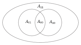
Figure 1. The Ven diagram for ${\mathcal{F}}_{d}^{2}$.

It is easily seen that for any solution $(p_{00},p_{01},p_{10},p_{11})$ of this system, we can immediately construct a pair of subsets $(A_{1},A_{2})\in{\mathcal{F}}_{d}\times{\mathcal{F}}_{d}$ by simply filling the sets $A_{00},A_{01},A_{10},A_{11}$ in the diagram of Figure 1 with $p_{00},p_{01},p_{10},p_{11}$ respective elements from the set $\Omega_{2d}$. Moreover, any two such fillings can be seen to be images of each other under suitable permutations of $S_{2d}$. In other words by this construction we obtain a bijection between the orbits of ${\mathcal{F}}_{d}\times{\mathcal{F}}_{d}$ under ${\mathcal{S}}_{2d}$ and the solutions of the system ${\mathcal{S}}_{2}$ we have previously encountered. This proves the theorem for $k=2$. The general case follows by an entirely analogous argument. ∎

Now we are ready to prove Theorem 1.2 and then Theorem 1.1.

Proof of Theorem 1.2.

We are to show that

$$m_{k}(d)=\big{\langle}h_{d,d}\odot h_{d,d}\odot\cdots\odot h_{d,d}\hskip 2.5pt,\hskip 2.5pts_{2d}\big{\rangle}.$$ (30)

It is well known that a transitive action of a group $G$ on a set $\Omega$ is equivalent to the action of $G$ on the left $G$-cosets of the stabilizer of any element of $\Omega$. In our case, pick the subset $[1,d]$ of $\Omega_{2d}$. Then the stabilizer is the Young subgroup $S_{[1,d]}\times S_{[d+1,2d]}$ of $S_{2d}$ and thus the Frobenius characteristic of this action is the homogeneous basis element $h_{d,d}=h_{d}h_{d}$. It follows then that the Frobenius characteristic of the action of $S_{2d}$ on the $k$-tuples $(A_{1},A_{2},\ldots,A_{k})$ of $d$-subsets of $\Omega_{2d}$ is given by the $k$-fold Kronecker product $h_{d,d}\odot h_{d,d}\odot\cdots\odot h_{d,d}.$ Therefore the scalar product

$$\big{\langle}h_{d,d}\odot h_{d,d}\odot\cdots\odot h_{d,d}\hskip 2.5pt,\hskip 2.5pts_{2d}\big{\rangle}$$

yields the multiplicity of the trivial under this action. But it is well known, and easy to see that this multiplicity is also equal to the number of orbits under this action. Thus (30) follows by Theorem 3.1. ∎

Proof of Theorem 1.1.

Again we will only need to do it for $k=2$. To this end note that by Theorem 1.2 the number of solutions of the system ${\mathcal{S}}_{2}^{1}$ in (29) is given by the scalar product

$$\big{\langle}h_{d,d}\odot h_{d,d}\hskip 2.5pt,\hskip 2.5pts_{2d}\big{\rangle}.$$ (31)

In the same vein we see that the number of solutions to the system ${\mathcal{S}}_{2}^{2}$ in (29) may be viewed as the number of orbits in the action of $S_{2d}$ on the pairs of subsets $(A_{1},A_{2})$ of $\Omega_{2d}$ where $|A_{2}|=|^{c}A_{2}|$ and $|A_{1}|=|^{c}A_{1}|+2$. We have seen that the Frobenius characteristic of the action of $S_{2d}$ on subsets of cardinality $d$ is $h_{d,d}$. On the other hand the action of $S_{2d}$ on sets of cardinality $d+1$ is equivalent to the action of $S_{2d}$ on left cosets of $S_{[1,d+1]}\times S_{[d+2,2d]}$ yielding that the Frobenius characteristic for this action is $h_{d+1}h_{d-1}$. Thus the Frobenius characteristic of the action of $S_{2d}$ on such pairs must be the Kronecker product

$$h_{d+1}h_{d-1}\odot h_{d}h_{d}.$$

It then follows that the number of solutions of the system ${\mathcal{S}}_{2}^{2}$ is given by the scalar product

$$\big{\langle}h_{d+1}h_{d-1}\odot h_{d}h_{d}\hskip 2.5pt,\hskip 2.5pts_{2d}\big{\rangle}.$$ (32)

The same reasoning gives that the number of solutions of the systems ${\mathcal{S}}_{2}^{3}$ and ${\mathcal{S}}_{2}^{4}$ in (29) are given by the scalar products

$$\big{\langle}h_{d}h_{d}\odot h_{d+1}h_{d-1}\hskip 2.5pt,\hskip 2.5pts_{2d}\big{\rangle}\enskip\enskip\hbox{and }\enskip\enskip\big{\langle}h_{d+1}h_{d-1}\odot h_{d+1}h_{d-1}\hskip 2.5pt,\hskip 2.5pts_{2d}\big{\rangle}.$$ (33)

It follows then that the coefficient of $q^{2d}$ in the alternating sum of formal power series in (27) is none other than the following alternating sum of the scalar products in (31), (32) and (33).

$$W_{2}(q)\Big{|}_{q^{2d}} =\big{\langle}h_{d}h_{d}\odot h_{d}h_{d}\hskip 2.5pt,\hskip 2.5pts_{2d}\big{\rangle}-\big{\langle}h_{d+1}h_{d-1}\odot h_{d}h_{d}\hskip 2.5pt,\hskip 2.5pts_{2d}\big{\rangle}$$

$$\qquad\qquad\qquad\qquad\qquad\qquad-\big{\langle}h_{d}h_{d}\odot h_{d+1}h_{d-1}\hskip 2.5pt,\hskip 2.5pts_{2d}\big{\rangle}+\big{\langle}h_{d+1}h_{d-1}\odot h_{d+1}h_{d-1}\hskip 2.5pt,\hskip 2.5pts_{2d}\big{\rangle}$$

$$=\big{\langle}\big{(}h_{d}h_{d}-h_{d+1}h_{d-1}\big{)}\odot\big{(}h_{d}h_{d}-h_{d+1}h_{d-1}\big{)}\hskip 2.5pt,\hskip 2.5pts_{2d}\big{\rangle}=\big{\langle}s_{d,d}\odot s_{d,d}\hskip 2.5pt,\hskip 2.5pts_{2d}\big{\rangle}.$$

Summing over $d$ gives

$$W_{2}(q)=\sum_{d\geq 0}q^{2d}\big{\langle}s_{d,d}\odot s_{d,d}\hskip 2.5pt,\hskip 2.5pts_{2d}\big{\rangle}.$$

An entirely analogous argument proves the general identity in (5). ∎

4. Enter divided difference operators

There is a truly remarkable approach to the solutions of a variety of constant term problems which exhibit the same types of symmetries of the Hdd and Sdd problems. We will introduce the approach in some simple cases first. We define the double of the Diophantine system

$${\mathcal{S}}_{2}=\left\|\enskip\begin{matrix}p_{1}+p_{2}-p_{3}-p_{4}=0\cr p_{1}-p_{2}+p_{3}-p_{4}=0\cr\end{matrix}\right.$$

to be the system

$${\mathcal{S}}{\mathcal{S}}_{2}=\bigg{\|}\enskip\begin{matrix}p_{1}+p_{2}-p_{3}-p_{4}\,+\,p_{5}+p_{6}-p_{7}-p_{8}=0\cr p_{1}-p_{2}+p_{3}-p_{4}\,+\,p_{5}-p_{6}+p_{7}-p_{8}=0\cr\end{matrix}.$$

As we can easily see we have simply repeated twice each linear form and appropriately increased the indices of the variables. Now suppose that we are in possession of the complete generating function of ${\mathcal{S}}_{2}$, that is

$$F_{{\mathcal{S}}_{2}}(x_{1},x_{2},x_{3},x_{4})=\sum_{p\in{\mathcal{S}}_{2}}x_{1}^{p_{1}}x_{2}^{p_{2}}x_{3}^{p_{3}}x_{4}^{p_{4}}.$$

We claim that the complete generating function of ${\mathcal{S}}{\mathcal{S}}_{2}$ is simply given by

$$F_{{\mathcal{S}}{\mathcal{S}}_{2}}(x_{1},x_{2},\ldots,x_{8})=\delta_{1,5}\delta_{2,6}\delta_{3,7}\delta_{4,8}F_{{\mathcal{S}}_{2}}(x_{1},x_{2},x_{3},x_{4}),$$ (34)

where for any pair of indices $(i,j)$ we let $\delta_{i,j}$ denote the divided difference operator defined for any function $f(x)$ by

$$\delta_{i,j}f(x)=\frac{f(x)-f(x)\big{|}_{x_{i}=x_{j},x_{j}=x_{i}}}{x_{i}-x_{j}}.$$

Proof of (34).

By MacMahon partition analysis we have

$$F_{{\mathcal{S}}_{2}}(x_{1},x_{2},x_{3},x_{4})={1\over(1-x_{1}a_{1}a_{2})}{1\over(1-x_{2}a_{1}/a_{2})}{1\over(1-x_{3}a_{2}/a_{1})}{1\over(1-x_{4}/a_{1}a_{2})}\hskip 2.5pt\bigg{|}_{a_{1}^{0}a_{2}^{0}}.$$ (35)

Now note that since

$$\delta_{1,5}{1\over(1-x_{1}a_{1}a_{2})} =\left({1\over(1-x_{1}a_{1}a_{2})}\,-\,{1\over(1-x_{5}a_{1}a_{2})}\right){1\over x_{1}-x_{5}}={a_{1}a_{2}\over(1-x_{1}a_{1}a_{2})(1-x_{5}a_{1}a_{2})},$$

we obtain similarly

$$\delta_{2,6}{1\over(1-x_{2}a_{1}/a_{2})}={a_{1}/a_{2}\over(1-x_{2}a_{1}/a_{2})(1-x_{6}a_{1}/a_{2})},$$

$$\delta_{3,7}{1\over(1-x_{3}a_{2}/a_{1})}={a_{2}/a_{1}\over(1-x_{3}a_{2}/a_{1})(1-x_{7}a_{2}/a_{1})},$$

$$\delta_{4,8}{1\over(1-x_{4}/a_{1}a_{2})}={1/a_{1}a_{2}\over(1-x_{4}/a_{1}a_{2})(1-x_{8}/a_{1}a_{2})}.$$

Thus applying the operator $\delta_{1,5}\delta_{2,6}\delta_{3,7}\delta_{4,8}$ to both sides of (35) gives

$$\delta_{1,5}\delta_{2,6}\delta_{3,7}\delta_{4,8}F_{{\mathcal{S}}_{2}}(x_{1},x_{2},x_{3},x_{4})={1\over(1-x_{1}a_{1}a_{2})(1-x_{2}a_{1}/a_{2})(1-x_{3}a_{2}/a_{1})(1-x_{4}/a_{1}a_{2})}\\ {\over(1-x_{5}a_{1}a_{2})(1-x_{6}a_{1}/a_{2})(1-x_{7}a_{2}/a_{1})(1-x_{8}/a_{1}a_{2})}\bigg{|}_{a_{1}^{0}a_{2}^{0}}.$$ (36)

Now we can easily recognize that (36) is precisely the constant term that MacMahon partition analysis would yield for the system ${\mathcal{S}}{\mathcal{S}}_{2}$. This proves (34). ∎

Note that to obtain the equality in (36) we have used the simple fact that the divided difference operator and the constant term operator do commute. This is the fundamental property which is at the root of the present algorithm. This example should make it evident to have the following more general result (with double modified).

Theorem 4.1.

If $F_{\mathcal{S}}(x_{1},x_{2},\ldots,x_{n})$ is the complete generating function of the Diophantine system

$${\mathcal{S}}=\left\|\ \begin{bmatrix}b_{11}&b_{12}&\cdots&b_{1n}\\ \vdots&\vdots&\cdots&\vdots\\ b_{r1}&b_{r2}&\cdots&b_{rn}\\ \end{bmatrix}\begin{bmatrix}p_{1}\\ \vdots\\ p_{n}\\ \end{bmatrix}=\begin{bmatrix}c_{1}\\ \vdots\\ c_{r}\\ \end{bmatrix}\right.,$$

then the complete generating function of the doubling of ${\mathcal{S}}$ defined by

$${\mathcal{S}}{\mathcal{S}}=\left\|\ \left[\begin{matrix}b_{11}&b_{12}&\cdots&b_{1n}\\ \vdots&\vdots&\cdots&\vdots\\ b_{r1}&b_{r2}&\cdots&b_{rn}\\ \end{matrix}\ \right|\left.\begin{matrix}b_{11}&b_{12}&\cdots&b_{1n}\\ \vdots&\vdots&\cdots&\vdots\\ b_{r1}&b_{r2}&\cdots&b_{rn}\\ \end{matrix}\right]\begin{bmatrix}p_{1}\\ \vdots\\ p_{2n}\\ \end{bmatrix}=\begin{bmatrix}c_{1}-b_{11}-b_{12}-\cdots-b_{1n}\\ \vdots\\ c_{r}-b_{r1}-b_{r2}-\cdots-b_{rn}\\ \end{bmatrix}\right.$$

is given by the rational function

$$F_{{\mathcal{S}}{\mathcal{S}}}(x_{1},x_{2},\dots,x_{2n})=\delta_{1,n+1}\delta_{2,n+2}\cdots\delta_{n,2n}F_{\mathcal{S}}(x_{1},x_{2},\ldots,x_{n}).$$

This result combined with the next simple observation yields a powerful algorithm for computing a variety of complete generating functions.

Theorem 4.2.

Let $F_{\mathcal{S}}(x_{1},x_{2},\ldots,x_{n})$ be the complete generating function of a Diophantine system ${\mathcal{S}}$ then the complete generating function $F_{{\mathcal{S}}{\mathcal{E}}}(x_{1},x_{2},\ldots,x_{n})$ of the system ${\mathcal{S}}{\mathcal{E}}$ obtained by adding the equation

$${\mathcal{E}}=\big{\|}\ r_{1}p_{1}+r_{2}p_{2}+\cdots+r_{n}p_{n}=s$$

to ${\mathcal{S}}$ is obtained by taking the constant term

$$F_{{\mathcal{S}}{\mathcal{E}}}(x_{1},x_{2},\ldots,x_{n})=a^{-s}F_{\mathcal{S}}(a^{r_{1}}x_{1},a^{r_{2}}x_{2},\ldots,a^{r_{n}}x_{n})\Big{|}_{a^{0}}.$$

Proof.

By assumption

$$F_{\mathcal{S}}(x_{1},x_{2},\ldots,x_{n})=\sum_{p\in{\mathcal{S}}}x_{1}^{p_{1}}x_{2}^{p_{2}}\cdots x_{n}^{p_{n}}.$$

Now we have

$$a^{-s}F_{\mathcal{S}}(a^{r_{1}}x_{1},a^{r_{2}}x_{2},\ldots,a^{r_{n}}x_{n})\Big{|}_{a^{0}} =\sum_{p\in{\mathcal{S}}}x_{1}^{p_{1}}x_{2}^{p_{2}}\cdots x_{n}^{p_{n}}a^{r_{1}p_{1}+r_{2}p_{2}+\cdots+r_{n}p_{n}-s}\Big{|}_{a^{0}}$$

$$=\sum_{p\in{\mathcal{S}}{\mathcal{E}}}x_{1}^{p_{1}}x_{2}^{p_{2}}\cdots x_{n}^{p_{n}}$$

$$=F_{{\mathcal{S}}{\mathcal{E}}}(x_{1},x_{2},\ldots,x_{n}).\hskip 36.135pt\hskip 36.135pt\hskip 36.135pt$$

∎

These two results provide us with algorithms for (at least in principle) computing all the Hdd series $G_{k}(q)$ as well as the Sdd series $W_{k}(q)$.

Algorithm 4.3 (Hdd Case).

1. Initially compute the complete generating function for the Hdd problem for $k=1$. That is, compute the constant term

   $$F_{1}(x_{1},x_{2})={1\over(1-x_{1}a)(1-x_{2}/a)}\hskip 2.5pt\Big{|}_{a^{0}}.$$

2. With $F_{k-1}(x_{1},\ldots,x_{2^{k-1}})$ from step $\bf b_{k-1})$, compute by divided difference

   $$FF_{{k-1}}(x_{1},\ldots,x_{2^{k}})=\delta_{1,1+2^{k-1}}\cdots\delta_{2^{k-1},2^{k}}F_{k-1}(x_{1},\ldots,x_{2^{k-1}}).$$

3. With $FF_{k-1}(x_{1},\ldots,x_{2^{k-1}})$ from step $\bf a_{k})$, compute the complete generating function for the Sdd problem for $k$ by the following constant term:

   $$F_{k}(x_{1},x_{2},\ldots,x_{2^{k}})=FF_{k-1}(ax_{1},ax_{2},\ldots,ax_{2^{k-1}},x_{2^{k-1}+1}/a,\ldots,x_{2^{k}}/a)\Big{|}_{a^{0}}.$$

This sequence of steps in Algorithm 4.3 can be terminated by replacing step $\bf b_{k})$ by

1. The $q$-generating function $G_{k}(q)$ is given by the constant term

   $$G_{k}(q)\enskip=\enskip F_{{\mathcal{S}}{\mathcal{S}}_{k-1}}(aq,aq,\ldots,aq,q/a,\ldots,q/a)\Big{|}_{a^{0}}.$$

The steps up to $\mathbf{b_{3})}$ can be carried out by hand. For further steps we need a computer, and to carry out step $\mathbf{b_{5})}$ by computer we have to introduce one more tool as we shall see. Unfortunately Step $\mathbf{b_{6})}$ appears beyond reach at the moment.

It will be instructive to see what the first several steps give.

1. $$F_{{\mathcal{S}}_{1}}(x_{1},,x_{2})={1\over 1-x_{1}x_{2}}.$$

2. $$F_{{\mathcal{S}}{\mathcal{S}}_{1}}(x_{1},x_{2},x_{3},x_{4})={(1-x_{1}x_{2}x_{3}x_{4})\over(1-x_{1}x_{2})(1-x_{2}x_{3})(1-x_{1}x_{4})(1-x_{3}x_{4})}.$$

3. $$F_{{\mathcal{S}}_{2}}(x_{1},x_{2},x_{3},x_{4}) \enskip=\enskip{(1-x_{1}x_{2}x_{3}x_{4})\over(1-a^{2}x_{1}x_{2})(1-x_{2}x_{3})(1-x_{1}x_{4})(1-x_{3}x_{4}/a^{2})}\Big{|}_{a^{0}}$$

   $$\enskip=\enskip{1\over(1-x_{2}x_{3})(1-x_{1}x_{4})}.$$

4. $$F_{{\mathcal{S}}{\mathcal{S}}_{2}}(x) ={(1-x_{1}x_{4}x_{5}x_{8})(1-x_{2}x_{3}x_{6}x_{7})\over(1-x_{1}x_{8})(1-x_{2}x_{7})(1-x_{3}x_{6})(1-x_{4}x_{5})(1-x_{1}x_{4})(1-x_{2}x_{3})(1-x_{6}x_{7})(1-x_{5}x_{8})}.$$

5. $$F_{{\mathcal{S}}_{3}}(x) ={(1-x_{1}x_{4}x_{5}x_{8})(1-x_{2}x_{3}x_{6}x_{7})\over(1-x_{1}x_{8})(1-x_{2}x_{7})(1-x_{3}x_{6})(1-x_{4}x_{5})}$$ (37)

   $$\enskip\enskip\enskip\enskip\enskip\enskip\enskip\enskip\enskip\enskip\enskip\enskip\qquad\times{1\over(1-a^{2}x_{1}x_{4})(1-a^{2}x_{2}x_{3})(1-x_{6}x_{7}/a^{2})(1-x_{5}x_{8}/a^{2})}\Big{|}_{a^{0}}.\enskip\enskip$$ (38)

We can compute this constant term in many ways. In particular we could use one of the MacMahon identities given by Andrews in [1]. But it is interesting to point out that our divided difference algorithm has already provided us (in step $\bf a_{2})$) a formula we can use in step $\bf b_{3})$. In fact, the output of step $\bf a_{2})$

$$F_{{\mathcal{S}}{\mathcal{S}}_{1}}(x_{1},x_{2},x_{3},x_{4})\enskip=\enskip{(1-x_{1}x_{2}x_{3}x_{4})\over(1-x_{1}x_{2})(1-x_{2}x_{3})(1-x_{1}x_{4})(1-x_{3}x_{4})}$$

is the complete generating function of the system $p_{1}-p_{2}+p_{3}-p_{4}=0$, so by MacMahon partition analysis we should also have

$$F_{{\mathcal{S}}{\mathcal{S}}_{1}}(x_{1},x_{2},x_{3},x_{4})\enskip=\enskip{1\over(1-ax_{1})(1-x_{2}/a)(1-ax_{3})(1-x_{4}/a)}\Big{|}_{a^{0}}.$$

This implies that

$${1\over(1-a^{2}x_{1}x_{4})(1-a^{2}x_{2}x_{3})(1-x_{6}x_{7}/a^{2})(1-x_{5}x_{8}/a^{2})}\bigg{|}_{a^{0}}$$

$$\hskip 36.135pt\hskip 36.135pt\hskip 36.135pt\hskip 36.135pt\enskip\enskip\enskip\enskip=\enskip{(1-x_{1}x_{2}x_{3}x_{4})\over(1-x_{1}x_{2})(1-x_{2}x_{3})(1-x_{1}x_{4})(1-x_{3}x_{4})}\Bigg{|}_{\begin{matrix}x_{1}{\rightarrow}x_{1}x_{4}\cr x_{3}{\rightarrow}x_{2}x_{3}\cr x_{2}{\rightarrow}x_{6}x_{7}\cr x_{4}{\rightarrow}x_{5}x_{8}\cr\end{matrix}}$$

$$\hskip 36.135pt\hskip 36.135pt\hskip 36.135pt\hskip 36.135pt\enskip\enskip\enskip\enskip=\enskip{(1-x_{1}x_{2}x_{3}x_{4}x_{5}x_{6}x_{7}x_{8})\over(1-x_{1}x_{4}x_{6}x_{7})(1-x_{6}x_{7}x_{2}x_{3})(1-x_{1}x_{4}x_{5}x_{8})(1-x_{2}x_{3}x_{5}x_{8})}.$$

Using this in (38) gives

$$F_{{\mathcal{S}}_{3}}(x_{1},\ldots,x_{8}) \enskip=\enskip{(1-x_{1}x_{4}x_{5}x_{8})(1-x_{2}x_{3}x_{6}x_{7})\over(1-x_{1}x_{8})(1-x_{2}x_{7})(1-x_{3}x_{6})(1-x_{4}x_{5})}$$

$$\enskip\enskip\enskip\enskip\enskip\enskip\enskip\enskip\enskip\enskip\enskip\enskip\enskip\enskip\enskip\enskip\enskip\enskip\enskip\times{(1-x_{1}x_{2}x_{3}x_{4}x_{5}x_{6}x_{7}x_{8})\over(1-x_{1}x_{4}x_{6}x_{7})(1-x_{6}x_{7}x_{2}x_{3})(1-x_{1}x_{4}x_{5}x_{8})(1-x_{2}x_{3}x_{5}x_{8})}$$

$$\enskip=\enskip{1-x_{1}x_{2}x_{3}x_{4}x_{5}x_{6}x_{7}x_{8}\over(1-x_{1}x_{8})(1-x_{2}x_{7})(1-x_{3}x_{6})(1-x_{4}x_{5})(1-x_{1}x_{4}x_{6}x_{7})(1-x_{2}x_{3}x_{5}x_{8})}.$$

Replacing all the $x_{i}$ by the single variable $q$, we thus obtain that

$$G_{1}(q)={1\over 1-q^{2}}\hskip 2.5pt,\hskip 2.5pt\enskip G_{2}(q)={1\over(1-q^{2})^{2}}\hskip 2.5pt,\hskip 2.5pt\enskip G_{3}(q)={1-q^{8}\over(1-q^{2})^{4}(1-q^{4})^{2}}\enskip=\enskip{1+q^{4}\over(1-q^{2})^{4}(1-q^{4})}.$$

Using the computer to carry out step $\bf b_{4}^{\prime})$ gives

$$G_{4}(q)={1+q^{2}+21q^{4}+36q^{6}+74q^{8}+86q^{10}+74q^{6}+36q^{14}+21q^{16}+q^{18}+q^{20}\over(1-q^{2})^{7}(1-q^{4})^{4}(1-q^{6})}.$$

We shall see later what else has to be done to obtain $G_{5}(q)$.

Our divided difference algorithm can also be adapted to compute the first 4 Sdd series as well. In fact, again due to the fact that divided difference operators commute with the constant term operators, we can also show that all the complete Sdd series can (in principle) be obtained by the following algorithm.

Algorithm 4.4 (Sdd Case).

1. Initially compute the complete generating function for the Sdd problem for $k=1$. That is, compute the constant term

   $$W_{1}(x_{1},x_{2})={1-a^{2}\over(1-x_{1}a)(1-x_{2}/a)}\hskip 2.5pt\Big{|}_{a^{0}}.$$

2. With $W_{k-1}(x_{1},\ldots,x_{2^{k-1}})$ from step $\bf b_{k-1})$, compute by divided difference

   $$WW_{{k-1}}(x_{1},\ldots,x_{2^{k}})=\delta_{1,1+2^{k-1}}\cdots\delta_{2^{k-1},2^{k}}W_{k-1}(x_{1},\ldots,x_{2^{k-1}}).$$

3. With $WW_{k-1}(x_{1},\ldots,x_{2^{k-1}})$ from step $\bf a_{k})$, compute the complete generating function for the Sdd problem for $k$ by the following constant term:

   $$W_{k}(x_{1},x_{2},\ldots,x_{2^{k}})=WW_{k-1}(ax_{1},ax_{2},\ldots,ax_{2^{k-1}},x_{2^{k-1}+1}/a,\ldots,x_{2^{k}}/a)(1-a^{2})\Big{|}_{a^{0}}.$$

Note that similarly as for the Hdd-case, the sequence of steps in Algorithm 4.4 can be terminated by replacing step $\bf b_{k})$ by

1. To obtain the generating function $W_{k}(q)$ compute the constant term

   $$W_{k}(q)=WW_{k-1}(aq,aq,\ldots,aq,q/a,\ldots,q/a)(1-a^{2})\Big{|}_{a^{0}}.$$

Only steps $\bf a_{1})$ and $\bf a_{2})$ can be carried out by hand. Though steps 3 and 4 are routine they are too messy to do by hand. But step 5 again needs further tricks to be carried out by computer. Step 6 appears beyond reach at the moment.

It will be instructive to see what some of these steps give.

1. $$W_{1}(x_{1},x_{2})={1-x_{2}^{2}\over 1-x_{1}x_{2}}.$$

2. $$WW_{1}(x_{1},\ldots,x_{4})={1-x_{2}^{2}-x_{2}x_{4}-x_{4}^{2}+x_{1}x_{2}^{2}x_{4}+x_{2}^{2}x_{3}x_{4}-x_{1}x_{2}x_{3}x_{4}+x_{1}x_{2}x_{4}^{2}+x_{2}x_{3}x_{4}^{2}-x_{1}x_{2}^{2}x_{3}x_{4}^{2}\over(1-x_{1}x_{2})(1-x_{3}x_{2})(1-x_{1}x_{4})(1-x_{3}x_{4})}.$$

3. $$W_{2}(x_{1},x_{2},x_{3},x_{4})={1-x_{2}x_{4}-x_{3}x_{4}+x_{4}^{2}\over(1-x_{1}x_{4})(1-x_{2}x_{3})}.$$

   This gives

   $$W_{2}(q)={1\over 1-q^{2}}.$$

4. $$WW_{2}(x_{1},\ldots,x_{8})={(large\enskip\enskip numerator)\over(1-x_{1}x_{4})(1-x_{1}x_{8})(1-x_{2}x_{3})(1-x_{2}x_{7})(1-x_{3}x_{6})(1-x_{4}x_{5})(1-x_{5}x_{8})(1-x_{6}x_{7})}.$$

5. $$W_{3}(x_{1},\ldots,x_{8})={(large\enskip\enskip numerator)\over(1-x_{1}x_{8})(1-x_{2}x_{7})(1-x_{3}x_{6})(1-x_{4}x_{5})(1-x_{1}x_{4}x_{6}x_{7})(1-x_{2}x_{3}x_{5}x_{8})}.$$

6. Notwithstanding the complexity of the previous results it turns out that to obtain $W_{3}(q)$ we need only compute the constant term

   $$W_{3}(q)={1\over(1-q^{2})}\times{1-a^{2}\over(1-q^{2}a^{2})(1-q^{2}/a^{2})}\bigg{|}_{a^{0}}.$$ (39)

   To this end we start by determining the coefficients $A$ and $B$ in the partial fraction decomposition

   $${(1-a^{2})a^{2}\over(1-q^{2}a^{2})(a^{2}-q^{2})}={1\over q^{2}}\,+\,{A\over 1-q^{2}a^{2}}+{B\over a^{2}-q^{2}}$$

   obtaining

   $$A ={(1-a^{2})a^{2}\over(a^{2}-q^{2})}\bigg{|}_{a^{2}=1/q^{2}}=\,{(1-1/q^{2})/q^{2}\over(1/q^{2}-q^{2})}=-{1\over q^{2}(1+q^{2})},$$

   $$B ={(1-a^{2})a^{2}\over(1-q^{2}a^{2})}\bigg{|}_{a^{2}=q^{2}}={(1-q^{2})q^{2}\over(1-q^{4})}={q^{2}\over(1+q^{2})},$$

   (the exact value of $B$ is not needed) and we can write

   $${1-a^{2}\over(1-q^{2}a^{2})(1-q^{2}/a^{2})}={1\over q^{2}}\,-\,{1\over q^{2}(1+q^{2})}\times{1\over(1-a^{2}q^{2})}\,+\,{1\over(1+q^{2})}\times{q^{2}/a^{2}\over 1-q^{2}/a^{2}}.$$

   Thus taking constant terms gives

   $${1-a^{2}\over(1-q^{2}a^{2})(1-q^{2}/a^{2})}\bigg{|}_{a^{0}}={1\over q^{2}}\,-\,{1\over q^{2}(1+q^{2})}\,+\,0={1\over 1+q^{2}}.$$

   Using this in (39) we finally obtain

   $$W_{3}(q)={1\over 1-q^{4}}.$$

7. $$WW_{4}(x_{1},x_{2},\ldots,x_{16})=(too\enskip large\enskip for\enskip typesetting)$$

8. Notwithstanding the complexity of the previous result it turns out that to obtain $W_{4}(q)$ we need only compute the constant term

   $$W_{4}(q)={(1+q^{4})(1+q^{6})\over(1-q^{2})(1-q^{4})^{2}}\times{1-a^{2}\over(1-a^{2}q^{4})(1-q^{4}/a^{2})(1-a^{4}q^{4})(1-q^{4}/a^{4})}\bigg{|}_{a^{0}}.$$

To illustrate the power and flexibility of the partial fraction algorithm we will carry this out by hand. The reader is referred to [3] for a brief tutorial on the use of this algorithm. In the next few lines we will strictly adhere to the notation and terminology given in [3].

To begin we note that we need only calculate the constant term

$$C(x)={1-a\over(1-ax)(1-x/a)(1-a^{2}x)(1-x/a^{2})}\bigg{|}_{a^{0}},$$ (40)

since we can write

$$W_{4}(q)={(1+q^{4})(1+q^{6})\over(1-q^{2})(1-q^{4})^{2}}\times C(q^{4}).$$ (41)

Now we have

$${1\over(1-a^{2}x)(1-x/a^{2})}={a^{2}\over(1-a^{2}x)(a^{2}-x)}={1\over 1-x^{2}}{1\over 1-a^{2}x}\,+\,{1\over 1-x^{2}}{x/a^{2}\over 1-x/a^{2}}.$$

Thus (40) may be rewritten in the form

$$C(x) ={1\over 1-x^{2}}\left({(1-a)\over(1-ax)(1-x/a)}{1\over 1-a^{2}x}\bigg{|}_{a^{0}}\,+\,{(1-a)\over(1-ax)(1-x/a)}{x/a^{2}\over 1-x/a^{2}}\bigg{|}_{a^{0}}\right).$$ (42)

Note that in the first constant term we have only one dually contributing term and on the second we have only one contributing term. This gives

$${(1-a)\over(1-ax)(1-x/a)}{1\over 1-a^{2}x}\bigg{|}_{a^{0}} ={(1-a)\over(1-ax)}{1\over 1-a^{2}x}\bigg{|}_{a=x}={(1-x)\over(1-x^{2})}{1\over 1-x^{3}}$$ (43)

$${(1-a)\over(1-ax)(1-x/a)}{x/a^{2}\over 1-x/a^{2}}\bigg{|}_{a^{0}} ={(1-a)\over(1-x/a)}{x/a^{2}\over 1-x/a^{2}}\bigg{|}_{a=1/x}={-(1-x)\over(1-x^{2})}{x^{2}\over 1-x^{3}}.$$ (44)

Using (43) and (44) in (42) we get

$$C(x)={1\over 1-x^{2}}\left({(1-x)\over(1-x^{2})}{1\over 1-x^{3}}\,-\,{(1-x)\over(1-x^{2})}{x^{2}\over 1-x^{3}}\right)={1-x\over(1-x^{2})(1-x^{3})}.$$

Together with (41), we get

$$W_{4}(q)={(1+q^{4})(1+q^{6})\over(1-q^{2})(1-q^{4})^{2}}\times{1-q^{4}\over(1-q^{8})(1-q^{12})}={1\over(1-q^{2})(1-q^{4})^{2}(1-q^{6})}.$$

We will see in section 4 what needs to be done to carry out step $\bf b^{\prime}_{5}$ on the computer.

The identities for $W_{2}(q),W_{3}(q),W_{4}(q)$ in (6) have also been derived in [3] by symmetric function methods from the relation (5). In fact, all three results in (6) are immediate consequences of the following deeper symmetric function identity. (for a proof see [3, Section 2].)

Theorem 4.5.

$$s_{d,d}\odot s_{d,d}=\sum_{\lambda\vdash 2d}s_{\lambda}\,\chi(\lambda\in EO_{4})$$

where $EO_{4}$ denotes the set of partitions of length $4$ whose parts are $\geq 0$ and all even or all odd.

Note that the Kronecker product identity

$$\big{\langle}s_{d,d}\odot s_{d,d}\odot s_{d,d}\odot s_{d,d}\odot s_{d,d}\hskip 2.5pt,\hskip 2.5pts_{2d}\big{\rangle}\enskip=\enskip\big{\langle}s_{d,d}\odot s_{d,d}\odot s_{d,d}\hskip 2.5pt,\hskip 2.5pts_{d,d}\odot s_{d,d}\big{\rangle}.$$

suggests obtaining $W_{5}(q)$ by means of a combinatorial interpretation of the coefficients of the Schur function expansion of the Kronecker product $s_{d,d}\odot s_{d,d}\odot s_{d,d}$. However, to this date no formula has been given for these coefficients, combinatorial or otherwise.

5. Solving the Hdd problem for $k=5$

This section is divided into four parts. In the first subsection we start with our computer findings and end by giving a combinatorial decomposition that works nicely to obtain $F_{3}(x)$. In the second subsection, this decomposition is described algebraically and, together with group actions, turned into manipulatory gyrations that will be used to extract $G_{5}(q)$ and $W_{5}(q)$ out of our computers. In the third subsection, by combining the idea of decomposition and the method of divided difference in Section 4, we give our best way that reduce the computation time for $G_{5}(q)$ and $W_{5}(q)$ down to a few minutes. In the final subsection, we give our first algorithm to obtain $G_{5}(q)$ and $W_{5}(q)$.

5.1. A combinatorial decomposition for $F_{3}(x)$

Our initial efforts at solving the Hdd an Sdd problems were entirely carried out by computer experimentation. After obtaining quite easily the series $G_{2}(q)$, $G_{3}(q)$, $G_{4}(q)$ and $W_{2}(q)$, $W_{3}(q)$, $W_{4}(q)$, all the computer packages available to us failed to directly deliver $G_{5}(q)$ and $W_{5}(q)$.

The computer data obtained for the Hdd problem for $k=2,3$ were combinatorially so revealing that we have been left with a strong impression that this problem should have a very beautiful combinatorial general solution. Only time will tell if this will ever be the case. To stimulate further research we will begin by reviewing our initial computer and manual combinatorial findings.

Recall that we denoted by ${\mathcal{F}}_{d}$ the collection of all $d$-subsets of the $2d$ element set $\Omega_{2d}$. We also showed (in Theorem 3.1) that the coefficient $m_{d}(k)$ in the series $G_{k}(q)=\sum_{d\leq 0}q^{2d}m_{d}(k)$ counts the number of orbits under the action of the symmetric group ${\mathcal{S}}_{2d}$ on the $k$-fold cartesian product ${\mathcal{F}}_{d}\times{\mathcal{F}}_{d}\times\cdots\times{\mathcal{F}}_{d}$. Denoting by $(A_{1},A_{2},\ldots,A_{k})$ a generic element of this cartesian product, then each orbit is uniquely determined by the $2^{k}$ cardinalities

$$p_{\epsilon_{1},\epsilon_{2},\cdots,\epsilon_{k}}=\big{|}A_{1}^{\epsilon_{1}}\cap A_{2}^{\epsilon_{2}}\cap\cdots\cap A_{k}^{\epsilon_{k}}\big{|}$$

where for each $1\leq i\leq k$ we set

$$A^{\epsilon_{i}}_{i}=\left\{\begin{array}[]{ll}\,\,\,A_{i}&\textrm{ if }\epsilon_{i}=0,\cr\ {}^{c}A_{i}&\textrm{ if }\epsilon_{i}=1.\end{array}\right.\hskip 36.135pt(\hbox{here $\ {}^{c}A_{i}=\Omega_{2d}/A_{i}$}).$$

It is also convenient to set $A_{\epsilon_{1},\epsilon_{2},\cdots,\epsilon_{k}}=A_{1}^{\epsilon_{1}}\cap A_{2}^{\epsilon_{2}}\cap\cdots\cap A_{k}^{\epsilon_{k}}.$ This given we have seen that the condition $(A_{1},A_{2},\ldots,A_{k})\in{\mathcal{F}}_{d}^{k}$ is equivalent to the Diophantine system

$${\mathcal{S}}_{k}=\left\|\ \begin{matrix}\sum_{\epsilon_{1}=0}^{1}\sum_{\epsilon_{2}=0}^{1}\cdots\sum_{\epsilon_{k}=0}^{1}(1-2\epsilon_{1})p_{\epsilon_{1},\epsilon_{2},\cdots,\epsilon_{k}}=0,\cr\sum_{\epsilon_{1}=0}^{1}\sum_{\epsilon_{2}=0}^{1}\cdots\sum_{\epsilon_{k}=0}^{1}(1-2\epsilon_{2})p_{\epsilon_{1},\epsilon_{2},\cdots,\epsilon_{k}}=0,\cr\vdots\enskip\enskip\enskip\enskip\enskip\enskip\enskip\vdots\enskip\enskip\enskip\enskip\enskip\enskip\enskip\vdots\enskip\enskip\enskip\enskip\enskip\enskip\enskip\vdots\enskip\enskip\enskip\enskip\enskip\enskip\enskip\vdots\enskip\enskip\enskip\enskip\enskip\enskip\enskip\enskip\enskip\vdots\cr\sum_{\epsilon_{1}=0}^{1}\sum_{\epsilon_{2}=0}^{1}\cdots\sum_{\epsilon_{k}=0}^{1}(1-2\epsilon_{k})p_{\epsilon_{1},\epsilon_{2},\cdots,\epsilon_{k}}=0,\cr\end{matrix}\right.$$

together with the condition $|\Omega_{2d}|=2d$, that is $\sum_{\epsilon_{1}=0}^{1}\sum_{\epsilon_{2}=0}^{1}\cdots\sum_{\epsilon_{k}=0}^{1}p_{\epsilon_{1},\epsilon_{2},\cdots,\epsilon_{k}}=2d.$

There are several algorithms available to solve such a system. See for instance [7, Chapter 4.6]. The algorithm we used for our computer experimentations is the MacMahon algorithm which has been recently implemented in MATHEMATICA by Andrews, Paule and Riese and in MAPLE by Xin using the partial fraction method of computing constant terms.

The former can be downloaded from the web site

http://www.risc.uni-linz.ac.at/research/combinat/software/Omega/

and the latter from the web site

http://www.combinatorics.net.cn/homepage/xin/maple/ell2.rar.

For computer implementation we found it more convenient to use the alternate notation adopted in Remark 2.5. That is

$${\mathcal{S}}_{k}=\left\|\ p_{1}V_{1}\,+\,p_{2}V_{2}\,+\,\cdots\,+\,p_{2^{k}}V_{2^{k}}=0\right..$$ (45)

These algorithms may yield quite a bit more than the number of solutions of such a system. For instance, in our case letting ${\mathcal{C}}_{k}$ denote the collection of solutions of the system ${\mathcal{S}}_{k}$, the “Omega package” of Andrews, Paule and Riese should, in principle, yield the formal power series

$$F_{k}(x_{1},x_{2},\ldots,x_{2^{k}})\,=\sum_{(p_{1},p_{2},\ldots,p_{2^{k}})\in\,{\mathcal{C}}_{k}}x_{1}^{p_{1}}x_{2}^{p_{2}}\cdots x_{2^{k}}^{p_{2^{k}}}.$$

It follows from the general theory of Diophantine systems that $F_{k}(x_{1},x_{2},\ldots,x_{2^{k}})$ is always the Taylor series of a rational function.

Now for ${\mathcal{S}}_{2}$ and ${\mathcal{S}}_{3}$ the Omega package gives

$$F_{2}(x_{1},x_{2},x_{3},x_{4}) ={1\over(1-x_{1}x_{4})(1-x_{2}x_{3})}$$ (46)

$$F_{3}(x_{1},x_{2},\ldots,x_{8}) ={1-x_{2}x_{3}x_{5}x_{8}x_{1}x_{4}x_{6}x_{7}\over(1-x_{1}x_{8})(1-x_{2}x_{7})(1-x_{3}x_{6})(1-x_{4}x_{5})(1-x_{2}x_{3}x_{5}x_{8})(1-x_{1}x_{4}x_{6}x_{7})}.$$ (47)

But this is as far as this package went in our computers. However we could go further by giving up full information about the solutions and only ask for the series

$$G_{k}(q)=F_{k}(x_{1},x_{2},\ldots,x_{2^{k}})\big{|}_{x_{i}=q},$$

which can be computed from its constant term representation in (8). For example, the program Latte by De Loera, Hemmecke, Tauzer, Yoshida, which is available at

http://www.math.ucdavis.edu /~latte/

computed the $G_{4}(q)$ series in approximately $30$ seconds. However, this is as far as Latte went on our machines. We should also mention that all the series $G_{k}(q)$ and $W_{k}(q)$ for $k\leq 4$ can be obtained in only a few seconds, from the software of Xin by computing the corresponding constant terms in (8) and (9).

To get our computers to deliver $G_{5}(q)$ and $W_{5}(q)$ in a matter of minutes a divide and conquer strategy had to be adopted. More precisely, these rational functions were obtained by decomposing the constant terms (8) and (9) as sums of constant terms. This decomposition had its origin from an effort to find a human proof of the identities in (46) and (47). More importantly, the surprising simplicity of (46) and (47) required a combinatorial explanation. Our findings there provided the combinatorial tools that were used in our early computations of $G_{5}(q)$ and $W_{5}(q)$. This given, before describing our work on these series, we will show how to obtain (46) and (47) entirely by hand.

Let us start by sketching the idea for $k=2$. Beginning with

$${\mathcal{S}}_{2}=\left\|\eqalign{&p_{1}+p_{2}-p_{3}-p_{4}=0\cr&p_{1}-p_{2}+p_{3}-p_{4}=0\cr}\right.$$

we immediately notice that $(1,0,0,1)$ and $(0,1,1,0)$ are solutions. Set

$$a=\min(p_{1},p_{4})\text{ and }b=\min(p_{2},p_{3}).$$

It is clear that the following difference must also be a solution.

$$(q_{1},q_{2},q_{3},q_{4})=(p_{1},p_{2},p_{3},p_{4})-(a,b,b,a)=(p_{1}-a,p_{2}-b,p_{3}-b,p_{4}-a).$$

Now $q_{1}q_{4}=0$ and $q_{2}q_{3}=0$. This gives us four possibilities for $(q_{1},q_{2},q_{3},q_{4})$:

$$(0,0,x,y)\hskip 2.5pt,\hskip 2.5pt\enskip(0,x,0,y)\hskip 2.5pt,\hskip 2.5pt\enskip(x,0,y,0)\hskip 2.5pt,\hskip 2.5pt\enskip(x,y,0,0),$$ (48)

for some nonnegative integers $x,y$. Testing the first equation of ${\mathcal{S}}_{2}$ immediately forces the first and last in (48) to identically vanish. Similarly, the second equation of ${\mathcal{S}}_{2}$ yields that the second and third in (48) must also identically vanish. This proves that the general solution of ${\mathcal{S}}_{2}$ is of the form $(a,b,b,a)$. We thus reobtain the full generating function (46) of solutions of ${\mathcal{S}}_{2}$:

$$F_{2}(x_{1},x_{2},x_{3},x_{4})=\sum_{a\geq 0}\sum_{b\geq 0}x_{1}^{a}x_{2}^{b}x_{3}^{b}x_{4}^{a}={1\over(1-x_{1}x_{4})(1-x_{2}x_{3})}.$$

It turns out that we can deal with ${\mathcal{S}}_{3}$ in a similar manner. Again we begin by noticing the four symmetric solutions

$$(1,0,0,0,0,0,0,1)\hskip 2.5pt,\hskip 2.5pt\enskip(0,1,0,0,0,0,1,0)\hskip 2.5pt,\hskip 2.5pt\enskip(0,0,1,0,0,1,0,0)\hskip 2.5pt,\hskip 2.5pt\enskip(0,0,0,1,1,0,0,0).$$

Next we set

$$a=\min(p_{1},p_{8}),\enskip b=\min(p_{2},p_{7}),\enskip c=\min(p_{3},p_{6}),\enskip d=\min(p_{4},p_{5}),\enskip$$

and by subtraction we get a solution

$$(q_{1},q_{2},q_{3},q_{4},q_{5},q_{6},q_{7},q_{8})=(p_{1},p_{2},p_{3},p_{4},p_{5},p_{6},p_{7},p_{8})-(a,b,c,d,d,c,b,a)$$ (49)

with the property $q_{i}q_{9-i}=0$ for $1\leq i\leq 4$. It will be good here and after to call the set

$$\{i\in[1,n]\,:\,p_{i}\geq 1\}$$

the support of the composition $(p_{1},p_{2},\ldots,p_{n})$. This given, we derive that the resulting composition in (49) will necessarily have its support contained in at least one of the following 16 patterns.

$$\eqalign{&(0,0,0,0,*,*,*,*)\hskip 2.5pt,\hskip 2.5pt\,(0,0,0,*,0,*,*,*)\hskip 2.5pt,\hskip 2.5pt\,(0,0,*,0,*,0,*,*)\hskip 2.5pt,\hskip 2.5pt\,(0,0,*,*,0,0,*,*)\hskip 2.5pt,\hskip 2.5pt\cr&(0,*,0,0,*,*,0,*)\hskip 2.5pt,\hskip 2.5pt\,(0,*,0,*,0,*,0,*)\hskip 2.5pt,\hskip 2.5pt\,(0,*,*,0,*,0,0,*)\hskip 2.5pt,\hskip 2.5pt\,(0,*,*,*,0,0,0,*)\hskip 2.5pt,\hskip 2.5pt\cr&(*,0,0,0,*,*,*,0)\hskip 2.5pt,\hskip 2.5pt\,(*,0,0,*,0,*,*,0)\hskip 2.5pt,\hskip 2.5pt\,(*,0,*,0,*,0,*,0)\hskip 2.5pt,\hskip 2.5pt\,(*,0,*,*,0,0,*,0)\hskip 2.5pt,\hskip 2.5pt\cr&(*,*,0,0,*,*,0,0)\hskip 2.5pt,\hskip 2.5pt\,(*,*,0,*,0,*,0,0)\hskip 2.5pt,\hskip 2.5pt\,(*,*,*,0,*,0,0,0)\hskip 2.5pt,\hskip 2.5pt\,(*,*,*,*,0,0,0,0).}$$ (54)

Unlike the case $k=2$ not all of these patterns force a trivial solution. To find out which it is helpful to resort to a Venn diagram imagery. To this end recall that a solution of ${\mathcal{S}}_{3}$ gives the cardinalities of the 8 regions of the Venn diagram of three $d$-subsets $A_{1},A_{2},A_{3}$ of $\Omega_{2d}$ (see Figure 2).

Figure 2. The Ven diagram for ${\mathcal{S}}_{3}$.

In Figure 3, each pattern is represented by a Venn diagram where in each region $A_{1}^{\epsilon_{1}}\cap A_{2}^{\epsilon_{2}}\cap A_{3}^{\epsilon_{3}}$ that corresponds to a $*$ in the pattern we placed a black dot. That means that only the regions with a dot may have $\geq 0$ cardinality. The miracle is that all but the two patterns $(0,*,*,0,*,0,0,*)$ and $(*,0,0,*,0,*,*,0)$ can be quickly excluded by a reasoning that only uses the positions of the dots in the Venn diagram. In fact, in each of the excluded cases, we show that it is impossible to replace the dots by $\geq 0$ integers in such a manner that the three sets $A_{1},A_{2},A_{3}$ and their complements $\ {}^{c}A_{1},\ ^{c}A_{2},\ ^{c}A_{3}$ end up having the same cardinality (except for all empty sets).

Figure 3. The 16 support patterns for ${\mathcal{S}}_{3}$.

The reasoning is so cute that we are compelled to present it here in full. In what follows the $j^{\mathrm{th}}$ diagram in the $i^{\mathrm{th}}$ row will be referred to as “$D_{ij}$”:

1. $D_{11}$, $D_{14}$, $D_{16}$, $D_{23}$, $D_{25}$, and $D_{28}$ can be immediately excluded because one of $A_{1}$, $A_{2}$, $A_{3}$, $A_{1}^{c}$, $A_{2}^{c}$ or $A_{3}^{c}$ would be empty.

2. In $D_{15}$ the dot next to 8 should give the cardinality of $A_{2}^{c}$ (say $d$) and then the dot next to the 2 should also give $d$. But that forces the dots next to 5 and 6 to be $0$, leaving $A_{3}$ empty, a contradiction. The same reasoning applies to $D_{12}$, $D_{13}$, $D_{18}$, $D_{21}$, $D_{24}$, $D_{26}$, and $D_{27}$.

That leaves only the two diagrams $D_{17}$ and $D_{22}$ which clearly correspond to the two above mentioned patterns. Now we see that for $D_{22}$ we must have the equalities $p_{1}+p_{4}=p_{1}+p_{6}=p_{1}+p_{7}=p_{6}+p_{7}.$ This forces $p_{1}=p_{4}=p_{6}=p_{7}$. In summary this pattern can only support the composition $(u,0,0,u,0,u,u,0)$. The same reasoning yields that the diagram $D_{17}$ can only support the composition $(0,v,v,0,v,0,0,v)$. It follows that the general solution of ${\mathcal{S}}_{3}$ must be of the form $(a,b,c,d,d,c,b,a)+(u,v,v,u,v,u,u,v).$

Now recall that after the subtraction of a symmetric solution we are left with an asymmetric solution. Thus to avoid over counting we must impose the condition $u\,v=0$. This leaves only three possibilities $u=v=0$, $u>0,v=0$ or $u=0,v>0$. Thus

$$F_{3}(x) =\sum_{a\geq 0}\sum_{b\geq 0}\sum_{c\geq 0}\sum_{d\geq 0}(x_{1}x_{8})^{a}(x_{2}x_{7})^{b}(x_{3}x_{6})^{c}(x_{4}x_{5})^{d}\Big{(}1\,+\,\sum_{u\geq 1}(x_{1}x_{4}x_{6}x_{7})^{u}\,+\,\sum_{v\geq 1}(x_{2}x_{3}x_{5}x_{8})^{v}\Big{)}$$

$$={1\over(1-x_{1}x_{8})(1-x_{2}x_{7})(1-x_{3}x_{6})(1-x_{4}x_{5})}\left(1\,+\,{x_{1}x_{4}x_{6}x_{7}\over 1-x_{1}x_{4}x_{6}x_{7}}\,+\,{x_{2}x_{3}x_{5}x_{8}\over 1-x_{2}x_{3}x_{5}x_{8}}\right).$$

which is only another way of writing (47).

5.2. Algebraic decompositions and group actions

It is easy to see that the decomposition of a solution into a sum of a symmetric plus an asymmetric solution can be carried out for general $k$. In fact, note that if $0\leq i\leq 2^{k}-1$ has binary digits $\epsilon_{1}\epsilon_{2}\cdots\epsilon_{k}$ then the binary digits of $2^{k}-1-i$ are $\overline{\epsilon}_{1}\overline{\epsilon}_{2}\cdots\overline{\epsilon}_{k}$ (with $\overline{\epsilon}=1-\epsilon$). Thus we see from (45) that in each equation $p_{i}$ and $p_{2^{k}+1-i}$ appear with opposite signs. This shows that for each $k\geq 2$ the system ${\mathcal{S}}_{k}$ has $2^{k-1}$ symmetric solutions, which may be symbolically represented by the monomials $x_{i}x_{i^{\prime}}$ for $i=1,\dots,2^{k-1}$, where we use (and will often use) $i^{\prime}$ to denote $2^{k}+1-i$ when $k$ is fixed.

Proceeding as we did for ${\mathcal{S}}_{2}$ and ${\mathcal{S}}_{3}$ we arrive at a unique decomposition of each solution of ${\mathcal{S}}_{k}$ into

$$(p_{1},p_{2},\ldots,p_{2^{k}})=(u_{1},u_{2},\ldots,u_{2},u_{1})\,+\,(q_{1},q_{2},\ldots,q_{2^{k}})$$

with the first summand symmetric and the second asymmetric, that is $u_{i}=u_{i^{\prime}}$ and $q_{i}q_{i^{\prime}}=0$ for $1\leq i\leq 2^{k-1}$, and thereby obtain a factorization of $F_{k}(x)$ in the form

$$F_{k}(x)=\bigg{(}\prod_{i=1}^{2^{k-1}}{1\over 1-x_{i}x_{i^{\prime}}}\bigg{)}F_{k}^{A}(x)$$ (55)

with $F_{k}^{A}(x)$ denoting the complete generating function of the asymmetric solutions.

This given it is tempting to try to apply, in the general case, the same process we used for $k=3$ and obtain the rational function $F_{k}^{A}(x)$ by selecting the patterns that do contain the support of an asymmetric solution. Note that the total number of asymmetric patterns to be examined is $2^{2^{k-1}}$ which is already $256$ for $k=4$. For $k=5$ the number grows to $65,536$ and doing this by hand is out of the question. Moreover, it is easy to see, by going through a few cases, that even for $k=4$ the geometry of the Venn Diagrams is so intricate that the only way that we can find out if a given pattern contains the support of a solution is to solve the corresponding reduced system.

Nevertheless, using some inherent symmetries of the problem, the complexity of the task can be substantially reduced to permit the construction of $G_{5}(q)$ by computer. To describe how this was done we need some notation. We will start with the complete generating function of the system ${\mathcal{S}}_{k}$ as given in Remark 2.5, that is

$$F_{k}(x_{1},x_{2},\ldots,x_{2^{k}})=\prod_{i=1}^{2^{k}}{1\over 1-x_{i}A_{i}}\hskip 2.5pt\bigg{|}_{a_{1}^{0}a_{2}^{0}\cdots a_{k}^{0}},$$

where $A_{i}=\prod_{i=1}^{k}a_{i}^{1-2\epsilon_{i}}$, with $\epsilon_{1}\epsilon_{2}\cdots\epsilon_{k}$ being the binary digits of $i-1$. Note that since (as we previously observed) the binary digits of $2^{k}-1-i$ are $\overline{\epsilon}_{1}\overline{\epsilon}_{2}\cdots\overline{\epsilon}_{k}$, we have $A_{i^{\prime}}=1/A_{i}.$ It then follows that

$${1-x_{i}x_{i^{\prime}}\over(1-x_{i}A_{i})(1-x_{i^{\prime}}A_{i^{\prime}})}=\left({1\over 1-x_{i}A_{i}}\,+\,{x_{i^{\prime}}/A_{i}\over 1-x_{i^{\prime}}/A_{i}}\right).$$

Thus combining the factors containing $A_{i}$ and $A_{i^{\prime}}$ we may rewrite (55) in the form

$$F_{k}(x_{1},x_{2},\ldots,x_{2^{k}})=\prod_{i=1}^{2^{k-1}}{1\over 1-x_{i}x_{i^{\prime}}}\prod_{i=1}^{2^{k-1}}\left({1\over(1-x_{i}A_{i})}\,+\,{x_{i^{\prime}}/A_{i}\over(1-x_{i^{\prime}}/A_{i})}\right)\hskip 2.5pt\bigg{|}_{a_{1}^{0}a_{2}^{0}\cdots a_{k}^{0}}.$$ (56)

Comparing with (55) we derive that the complete generating function of the asymmetric solutions is given by the following sum.

$$F_{k}^{A}(x)=\sum_{S\subseteq[1,2^{k-1}]}F_{S}(x),$$ (57)

where

$$F_{S}(x)=\bigg{(}\prod_{i\notin S}{1\over(1-x_{i}A_{i})}\bigg{)}\times\bigg{(}\prod_{i\in S}{x_{i^{\prime}}/A_{i}\over(1-x_{i^{\prime}}/A_{i})}\bigg{)}\hskip 2.5pt\bigg{|}_{a_{1}^{0}a_{2}^{0}\cdots a_{k}^{0}}.$$ (58)

In this way we have described our decomposition algebraically. Using notation as of (45), we can see that $F_{S}(x)$ is none other than the complete generating function of the reduced system

$$\sum_{i\notin S}p_{i}V_{i}\hskip 2.5pt\,+\,\hskip 2.5pt\sum_{i\in S}p_{i^{\prime}}V_{i^{\prime}}=0$$

with the added condition that $p_{i^{\prime}}\geq 1$ for all $i\in S.$

Note that for $k=3$ the summands in (57) correspond precisely to the $16$ patterns in (54) with the added condition that the “$*$” in position $i\geq 5$ should represent $p_{i}\geq 1$ in the corresponding solution vector. This extra condition is precisely what is needed to eliminate overcounting.

Perhaps all this is best understood with an example. For instance for $k=3$ the patterns

$$(*,0,0,*,0,*,*,0)\enskip\enskip\enskip\hbox{and }\enskip\enskip\enskip(0,*,*,0,*,0,0,*)$$

were the only ones that supported an asymmetric solution represent the two reduced systems

$${\mathcal{S}}_{\{14\}}=\bigg{\|}\begin{matrix}&p_{1}+p_{4}-p_{6}-p_{7}=0\cr&p_{1}-p_{4}+p_{6}-p_{7}=0\cr&p_{1}-p_{4}-p_{6}+p_{7}=0\cr\end{matrix}\hskip 36.135pt{\mathcal{S}}_{\{23\}}=\bigg{\|}\begin{matrix}&p_{2}+p_{3}-p_{5}-p_{8}=0\cr&p_{2}-p_{3}+p_{5}-p_{8}=0\cr&-p_{2}+p_{3}+p_{5}-p_{8}=0\cr\end{matrix}$$

and correspond to the following two summands of (57) for $k=3$

$$F_{\{1,4\}}(x) ={1\over 1-x_{1}a_{1}a_{2}a_{3}}{1\over 1-x_{4}a_{1}/a_{2}a_{3}}{x_{6}a_{2}/a_{1}a_{3}\over 1-x_{6}a_{2}/a_{1}a_{3}}{x_{7}a_{3}/a_{1}a_{2}\over 1-x_{7}a_{3}/a_{1}a_{2}}\hskip 2.5pt\bigg{|}_{a_{1}^{0}a_{2}^{0}a_{3}^{0}}={x_{1}x_{4}x_{6}x_{7}\over 1-x_{1}x_{4}x_{6}x_{7}}$$ (59)

$$F_{\{2,3\}}(x) ={1\over 1-x_{2}a_{1}a_{2}/a_{3}}{1\over 1-x_{3}a_{1}a_{3}/a_{2}}{x_{5}a_{2}a_{3}/a_{1}\over 1-x_{5}a_{2}a_{3}/a_{1}}{x_{8}/a_{1}a_{2}a_{3}\over 1-x_{8}/a_{1}a_{2}a_{3}}\hskip 2.5pt\bigg{|}_{a_{1}^{0}a_{2}^{0}a_{3}^{0}}\!\!\!={x_{2}x_{3}x_{5}x_{8}\over 1-x_{2}x_{3}x_{5}x_{8}}.$$ (60)

A close look at these two expressions should reveal the key ingredient that needs to be added to our algorithms that will permit reaching $k=5$ in the Hdd and Sdd problems. Indeed we see that $F_{\{1,4\}}(x)$ goes onto $F_{\{2,3\}}(x)$ if we act on the vector $(x_{1},x_{2},\cdots,x_{8})$ by the permutation

$$\sigma=\left(\begin{matrix}1&2&3&4&5&6&7&8\cr 3&4&1&2&7&8&5&6\cr\end{matrix}\right)$$ (61)

and on the triple $(a_{1},a_{2},a_{3})$ by the operation $a_{2}{\rightarrow}a_{2}^{-1}$. In fact, $\sigma$ is none other than an image of the map $(\epsilon_{1},\epsilon_{2},\epsilon_{3}){\rightarrow}(\epsilon_{1},\overline{\epsilon}_{2},\epsilon_{3})$ on the binary digits of $0,1,\ldots,7$, as we can easily see when we replace each $i$ in (61) by the binary digits of $i-1$

$$\sigma=\left(\begin{matrix}000&001&010&011&100&101&110&111\cr 010&011&000&001&110&111&100&101\cr\end{matrix}\right).$$

What goes on is quite simple. Recall that solutions $p$ of our system ${\mathcal{S}}_{k}$ can also be viewed as assignments of weights to the vertices of the $k$-hypercube giving all hyperfaces equal weight. Then clearly any rotation or reflection of the hypercube will carry this assignment onto an assignment with the same property. Thus the Hyperoctahedral group ${\mathcal{B}}_{k}$ will act on all the constructs we used to solve ${\mathcal{S}}_{k}$.

To make precise the action of ${\mathcal{B}}_{k}$ on $[1,2^{k}]$ we need some conventions.

1. We will view the elements of ${\mathcal{B}}_{k}$ as pairs $(\alpha,\eta)$ with a permutation $\alpha=(\alpha_{1},\alpha_{2},\ldots\alpha_{k})\in S_{k}$ and a binary vector $\eta=(\eta_{1},\eta_{2},\ldots,\eta_{k})$.

2. Next, for any binary vector $\epsilon=(\epsilon_{1},\epsilon_{2},\ldots,\epsilon_{k})$ let us set

   $$(\alpha,\eta)\epsilon=(\epsilon_{\alpha_{1}}+\eta_{1},\epsilon_{\alpha_{2}}+\eta_{2},\cdots,\epsilon_{\alpha_{k}}+\eta_{k})$$ (62)

   with “mod 2 ” addition.

3. This given, to each element $g=(\alpha,\eta)\in{\mathcal{B}}_{k}$ there corresponds a permutation $\sigma(g)$ by setting

   $$\sigma(g)=\left(\begin{matrix}1&2&\cdots&{2^{k}}\cr\sigma_{1}&\sigma_{2}&\cdots&\sigma_{2^{k}}\cr\end{matrix}\right).$$

   where $\sigma_{i}=j$ if and only if the $k$-vector $\epsilon=(\epsilon_{1},\epsilon_{2},\ldots,\epsilon_{k})$ giving the binary digits of $i-1$ is sent by (62) onto the $k$-vector giving the binary digits of $j-1$. In particular we will set

   $$g(x_{1},x_{2},\ldots,x_{2^{k}})=(x_{\sigma_{1}},x_{\sigma_{2}},\ldots,x_{\sigma_{2^{k}}}).$$ (63)

4. In the same vein we will make ${\mathcal{B}}_{k}$ act on the $k$-tuple $(a_{1},a_{2},\ldots,a_{k})$ by setting, again for $g=(\alpha,\eta)$

   $$g(a_{1},a_{2},\ldots,a_{k})=(a_{\alpha_{1}}^{1-2\eta_{1}},a_{\alpha_{2}}^{1-2\eta_{2}},\ldots,a_{\alpha_{k}}^{1-2\eta_{k}}).$$ (64)

With these conventions we can easily derive that $gx_{i}A_{i}=x_{\sigma_{i}}A_{\sigma_{i}}.$ Thus

$$g\prod_{i=1}^{2^{k}}{1\over 1-x_{i}A_{i}}\hskip 2.5pt\bigg{|}_{a_{1}^{0}a_{2}^{0}\cdots a_{k}^{0}}=\prod_{i=1}^{2^{k}}{1\over 1-x_{\sigma_{i}}A_{\sigma_{i}}}\hskip 2.5pt\bigg{|}_{a_{1}^{0}a_{2}^{0}\cdots a_{k}^{0}}=\prod_{i=1}^{2^{k}}{1\over 1-x_{i}A_{i}}\hskip 2.5pt\bigg{|}_{a_{1}^{0}a_{2}^{0}\cdots a_{k}^{0}}\hskip 2.5pt,$$

from which we again derive the ${\mathcal{B}}_{k}$ invariance of the complete generating function $F_{k}(x_{1},x_{2},\ldots,x_{2^{k}}).$

If we let ${\mathcal{B}}_{k-1}$ not only act on the indices $1,2,\ldots,2^{k-1}$, but also on $1^{\prime},2^{\prime},\ldots,{2^{k-1}}^{\prime}$ by $\sigma_{i^{\prime}}=\sigma_{i}^{\prime}$. Then ${\mathcal{B}}_{k-1}$ permutes the summands in (57) as well as the factors in the product

$$\prod_{i=1}^{2^{k-1}}\!\!{1\over 1-x_{i}x_{i^{\prime}}}.$$

Note further that if we only want the $q$-series $G_{k}(q)$ we can reduce (57) to

$$G_{k}^{A}(q)=\sum_{S\subseteq[1,2^{k-1}]}G_{S}(q),$$ (65)

where $G_{S}(q)=F_{S}(x)\big{|}_{x_{i}=q}$. But if for some $g\in{\mathcal{B}}_{k-1}$ we have

$$F_{S_{1}}(x_{\sigma_{1}},x_{\sigma_{2}},\ldots,x_{\sigma_{2^{k}}})\enskip=\enskip F_{S_{2}}(x_{1},x_{2},\ldots,x_{{2^{k}}}),$$

then replacing each $x_{i}$ by $q$ converts this to the equality $G_{S_{1}}(q)=G_{S_{2}}(q).$ That means that we need only compute the constant terms in (65) for orbit representatives, then replace (65) by a sum over orbit representatives multiplied by orbit sizes. More precisely we get

$$G_{k}^{A}(q)=\sum_{i}m_{i}G_{S_{i}}(q),$$ (66)

where the sum ranges over all orbits and $m_{i}$ denotes the cardinality of the orbit of the representative $F_{S_{i}}(x)$. In the computer implementation we obtain orbit representatives as well as orbit sizes, by acting with ${\mathcal{B}}_{k-1}$ on the monomials $M_{S}=\prod_{i\in S}x_{i}.$

Thus for $k=3$ we found that the $16$ summands in (57) break up into $6$ orbits but only $2$ of them do contribute to $F^{A}_{3}$. They corresponds to the monomials $1$ and $x_{1}x_{4}$ with respective orbit sizes $1$ and $2$. The orbit representative that corresponds to $1$ is simply the case $S=\phi$ in (58) and that corresponds to $x_{1}x_{4}$ is given in (59).

Thus from (59), (66) and (56) we derive (again) that

$$G_{3}(q)\enskip=\enskip{1\over(1-q^{2})^{4}}\Big{(}1+2{q^{4}\over 1-q^{4}}\Big{)}\enskip=\enskip{1\over(1-q^{2})^{4}}{1+q^{4}\over 1-q^{4}}.$$

For $k=4$ we have $2^{8}=256$ summands in (57) with $22$ orbits but only $11$ of these orbits do contribute to $F^{A}_{4}$. The number of denominator factors for each term is $8$ which is still a reasonable number for the partial fraction algorithm. The formula for $F_{4}(x)$ obtained this way can be typed within a page, but we would like to introduce a nicer $F_{4}(x)$ using the full group ${\mathcal{B}}_{k}$ instead of ${\mathcal{B}}_{k-1}$, as we will do in the next paragraph. For $k=5$ we have $2^{16}$ summands in (57) with $402$ orbits but only $341$ orbits do contribute to $F^{A}_{5}$. The number of denominator factors for each term is $16$ which is out of reach for the partial fraction algorithm to obtain $F^{A}_{5}(x)$. Nevertheless, in this manner we can still produce $G_{5}(q)$ in about 15 minutes.

The decomposition in (65) is only ${\mathcal{B}}_{k-1}$ invariant, and it is natural from the geometry of the hypercube labelings, to ask of a ${\mathcal{B}}_{k}$ invariant decomposition. To obtain such a decomposition of $F_{k}(x)$ we will pair off the factors containing $A_{i}$ and $A_{i^{\prime}}$ by means of the more symmetric identity

$${1-x_{i}x_{2^{k}+1-i}\over(1-x_{i}A_{i})(1-x_{2^{k}+1-i}A_{2^{k}+1-i})}=\left(1\,+\,{x_{i}A_{i}\over 1-x_{i}A_{i}}\,+\,{x_{i^{\prime}}A_{i^{\prime}}\over 1-x_{i^{\prime}}A_{i^{\prime}}}\right)$$

and derive that

$$F_{k}(x)=\sum_{S\cup T\subseteq[1,2^{k-1}]}F_{S,T}(x),$$

where $S$ and $T$ are disjoint and

$$F_{S,T}(x)=\bigg{(}\prod_{i\in S}^{k}{x_{i}A_{i}\over 1-x_{i}A_{i}}\bigg{)}\bigg{(}\prod_{i\in T}{x_{i}^{\prime}/A_{i}\over 1-x_{i}^{\prime}/A_{i}}\bigg{)}.$$

Note that every pair $(S,T)$ should be identified with the set $S\cup\{i^{\prime}:i\in T\}\subseteq[1,2^{k}]$ when applying the action of ${\mathcal{B}}_{k}$.

Example 5.1.

For $k=3$ we have $3^{4}=81$ summands with $9$ orbits but only $2$ orbits do contribute to $F^{A}_{3}$. The two orbits corresponds to the monomials $1$ and $x_{1}x_{4}x_{6}x_{7}$ with respective orbit sizes $1$ and $2$. The orbit representative that corresponds to $1$ is simply the case $F_{\phi,\phi}=1|_{a_{1}^{0}a_{2}^{0}a_{3}^{0}a_{4}^{0}}=1$ and that corresponds to $x_{1}x_{4}x_{6}x_{7}$ is

$$F_{\{1,4\},\{2,3\}}(x)={x_{1}A_{1}\over 1-x_{1}A_{1}}{x_{4}A_{4}\over 1-x_{4}A_{4}}{x_{6}A_{6}\over 1-x_{6}A_{6}}{x_{7}A_{7}\over 1-x_{7}A_{7}}\Big{|}_{a_{1}^{0}a_{2}^{0}a_{3}^{0}a_{4}^{0}}={x_{1}x_{4}x_{6}x_{7}\over 1-x_{1}x_{4}x_{6}x_{7}}.$$

Therefore, we can reobtain $G_{3}(q)$ by using (66) as follows.

$$G_{3}(q)=\frac{1}{(1-q^{2})^{4}}(1+\frac{2q^{4}}{1-q^{4}})=\frac{1+q^{4}}{(1-q^{2})^{4}(1-q^{4})}.$$

Example 5.2.

For $k=4$ we have $3^{8}=6561$ summands with $62$ orbits but only $10$ orbits do contribute to $F^{A}_{4}$. We obtain the following complete generating functions for the $10$ orbit representatives:

$$(1)\enskip 1$$

$$(24)\enskip{x_{1}x_{15}x_{4}x_{14}\over 1-x_{1}x_{15}x_{4}x_{14}}$$

$$(16)\enskip{x_{16}x_{7}\left({x_{9}}\right)^{2}x_{6}x_{4}\over 1-x_{16}x_{7}{x_{9}}^{2}x_{6}x_{4}}$$

$$(96)\enskip{x_{15}x_{3}x_{7}\left({x_{12}}\right)^{2}\left({x_{9}}\right)^{2}\left({x_{6}}\right)^{3}\over\left({1-x_{12}x_{7}x_{9}x_{6}}\right)\left({1-x_{15}x_{3}x_{12}x_{9}{x_{6}}^{2}}\right)}$$

$$(96)\enskip{x_{16}x_{14}x_{5}x_{7}\left({x_{11}}\right)^{2}\left({x_{2}}\right)^{2}\over\left({1-x_{2}x_{7}x_{11}x_{14}}\right)\left({1-x_{16}x_{5}x_{2}x_{11}}\right)}$$

$$(192)\enskip{x_{9}x_{10}x_{1}\left({x_{4}}\right)^{4}\left({x_{15}}\right)^{3}\left({x_{5}}\right)^{2}\left({x_{14}}\right)^{2}\over\left({1-x_{1}x_{15}x_{4}x_{14}}\right)\left({1-x_{15}x_{5}x_{10}x_{4}}\right)\left({1-x_{15}x_{5}x_{9}{x_{4}}^{2}x_{14}}\right)}$$

$$(64)\enskip{x_{6}x_{16}x_{4}\left({x_{3}}\right)^{2}\left({x_{5}}\right)^{2}\left({x_{15}}\right)^{2}\left({x_{10}}\right)^{3}\over\left({1-x_{15}x_{5}x_{10}x_{4}}\right)\left({1-x_{16}x_{5}x_{3}x_{10}}\right)\left({1-x_{15}x_{3}x_{10}x_{6}}\right)}$$

$$(64)\enskip{x_{3}x_{7}x_{4}\left({x_{6}}\right)^{5}x_{1}\left({x_{9}}\right)^{3}\left({x_{12}}\right)^{3}\left({x_{15}}\right)^{3}\over\left({1-x_{1}x_{15}x_{12}x_{6}}\right)\left({1-x_{12}x_{7}x_{9}x_{6}}\right)\left({1-x_{15}x_{9}x_{6}x_{4}}\right)\left({1-x_{15}x_{3}x_{12}x_{9}{x_{6}}^{2}}\right)}$$

$$(32)\enskip{\left({x_{13}}\right)^{3}\left({x_{12}}\right)^{3}x_{1}x_{3}x_{2}x_{6}x_{7}x_{8}\left({1-x_{1}x_{2}x_{3}x_{8}{x_{12}}^{3}x_{7}{x_{13}}^{3}x_{6}}\right)\over\left({1-x_{1}x_{8}x_{12}x_{13}}\right)\left({1-x_{2}x_{12}x_{7}x_{13}}\right)\left({1-x_{3}x_{12}x_{13}x_{6}}\right)\left({1-x_{1}{x_{12}}^{2}x_{7}x_{13}x_{6}}\right)\left({1-x_{2}x_{3}x_{8}x_{12}{x_{13}}^{2}}\right)}$$

$${(8)\enskip\enskip x_{4}x_{5}x_{3}x_{6}x_{9}x_{10}x_{15}x_{16}\left({1-2\,x_{15}x_{16}x_{5}x_{3}x_{10}x_{9}x_{6}x_{4}+{x_{15}}^{2}{x_{16}}^{2}{x_{5}}^{2}{x_{3}}^{2}{x_{10}}^{2}{x_{9}}^{2}{x_{6}}^{2}{x_{4}}^{2}}\right)\over\left({1-x_{16}x_{3}x_{9}x_{6}}\right)\left({1-x_{16}x_{5}x_{9}x_{4}}\right)\left({1-x_{15}x_{9}x_{6}x_{4}}\right)\left({1-x_{15}x_{5}x_{10}x_{4}}\right)\left({1-x_{16}x_{5}x_{3}x_{10}}\right)\left({1-x_{15}x_{3}x_{10}x_{6}}\right)}$$

Here the numbers in parentheses give the respective orbit sizes.

Replacing all the $x_{i}$ by $q$ and summing as in (66), we obtain

$$G_{4}(q)={1+q^{2}+21q^{4}+36q^{6}+74q^{8}+86q^{10}+74q^{12}+36q^{14}+21q^{16}+q^{18}+q^{20}\over(1-q^{2})^{7}(1-q^{4})^{4}(1-q^{6})}.$$

We should mention that the partial fraction algorithm delivers this rational function in less than a second by directly computing the constant term in (8) for $k=4$. We computed the above representatives because it contains more information and can be used for an alternate path to $G_{5}(q)$.

Computing the orbit representatives for $k=5$ requires the construction of the $2^{5}\times 5!=3840$ elements of ${\mathcal{B}}_{5}$ and examining their action on the $3^{16}=43046721$ symmetric supports. This took a few hours on our computers. We found in this manner that the $43046721$ summands in (65) break up into $15418$ orbits and of these $6341$ contribute to the sum. Most of the orbits have denominators of less than $16$ factors. It also took about $15$ minutes to persuade MAPLE to deliver $G_{5}(q)$ in the form displayed in the introduction.

It turns out that the same orbit reduction idea can also be used to compute $W_{5}(q)$, but much more complicated. Let us explain the details in the next subsection.

Remark 5.3.

It is interesting to point out that computing complete generating functions for orbit representatives of summands in (57) yielded as a byproduct orbit representatives of the extreme rays of our Diophantine cone for $k=4$ and $k=5$. Note that for $k=3$ the representatives can be directly derived from our hand computation, there are only two and the corresponding Venn Diagrams are

Here the regions without numbers are empty. The number $1$ indicates that the region has only one element. For $k=4$ we found that there are only three orbits, containing $24,8$ and $16$ elements respectively, the corresponding diagrams are depicted below.

Note, for $k=4$ each Venn diagram is depicted as a pair of Venn diagrams of $k=3$. The first member of the pair renders the Venn diagram of $A_{1}\cap A_{2},A_{1}\cap A_{3},A_{1}\cap A_{4}$ and the second member renders the Venn diagram of $\ {}^{c}A_{1}\cap A_{2},\ ^{c}A_{1}\cap A_{3},\ ^{c}A_{1}\cap A_{4}$.

For $k=5$ we found that there are $2712$ extreme rays which break up into $9$ orbits. We give in Figure 4 a set of representatives depicted as assignments of weights to the vertices of the $5$ dimensional hypercube. We imagine that the vertices of this hypercube are indexed by the binary digits of $0,1,2,\ldots,31$ with $00000$ the vertex at the origin and $11111$ giving the coordinates of the opposite vertex. In Figure 4 each hypercube is represented by two rows of two cubes. The cubes in the first row, from left to right, have the vertices labeled with the binary digits of 1 to 16 (minus 1) and the cubes in the second row have the vertices labeled with the binary digits of 17 to 32 (minus 1). The vertices here have possible weights $0,1,2,3$ and, correspondingly, are surrounded by $0,1,2,3$ concentric circles. The integer on the top of each diagram gives the size of the corresponding orbit.

Figure 4. Representatives of extreme rays for $k=5$.

Each of the corresponding solutions of our system ${\mathcal{S}}_{5}$ is minimal, that is, it cannot be decomposed into a non-trivial sum of solutions. But we found that there are also $480$ minimal solutions that do not come from extreme rays. The latter break up into two orbits, with representatives depicted in Figure 5.

Figure 5. Representatives for minimal solutions but not extreme rays.

5.3. Our fastest way for $G_{5}(q)$ and $W_{5}(q)$

With the notations in the previous subsection and Section 4 handy, we can describe our best way to obtain $G_{5}(q)$ and $W_{5}(q)$.

Let us explain the idea for $k=5$. In Example 5.2 we have obtained for $F_{4}^{A}(x)$ 10 orbit representatives with corresponding orbit sizes. Denote them by $R_{i}(x)$ the representatives and $m_{i}$ the orbit sizes for $i=1,\dots,10$. From this we can give explicit formula of $F_{4}^{A}(x)$ and hence of $F_{4}(x)$ with the help of ${\mathcal{B}}_{4}$ action as follows.

$$F_{4}(x)=\frac{F_{4}^{A}(x)}{\prod_{i=1}^{8}(1-x_{i}x_{17-i})}=\sum_{i=1}^{10}\frac{m_{i}}{|{\mathcal{B}}_{4}|}\sum_{g\in{\mathcal{B}}_{4}}g\frac{R_{i}}{\prod_{i=1}^{8}(1-x_{i}x_{17-i})}$$ (67)

Applying Algorithm 4.3 $\mathbf{a_{5}),b_{5})}$ to (67), we can obtain $F_{5}(x)$ by multilinearity.

$$F_{5}(x)=\sum_{i=1}^{10}\frac{m_{i}}{|{\mathcal{B}}_{4}|}\sum_{g\in{\mathcal{B}}_{4}}\left(g\delta_{1,17}\cdots\delta_{16,32}\frac{R_{i}}{\prod_{i=1}^{8}(1-x_{i}x_{17-i})}\right)\bigg{|}^{j=1,2,\dots,16}_{x_{j}=x_{j}a,x_{16+j}=x_{16+j}/a}\Bigg{|}_{a^{0}},$$ (68)

where we have used the straightforwardly checked fact: for any rational function $R(x_{1},\dots,x_{16})$ and $g\in{\mathcal{B}}_{k}$, it holds that

$$\delta_{1,17}\cdots\delta_{16,32}\;gR(x_{1},\dots,x_{16})=g\delta_{1,17}\cdots\delta_{16,32}R(x_{1},\dots,x_{16}),$$

where $g$ is extended to permute also indices $16+j$ by $g(16+j)=16+g(j)$ for $j=1,\dots,16$.

Substituting $x_{j}=q$ for all $j$ into (68) gives

$$G_{5}(q)=\sum_{i=1}^{10}m_{i}\left(\delta_{1,17}\cdots\delta_{16,32}\frac{R_{i}}{\prod_{i=1}^{8}(1-x_{i}x_{17-i})}\right)\bigg{|}^{j=1,2,\dots,16}_{x_{j}=x_{j}a,x_{16+j}=x_{16+j}/a}\ \Bigg{|}_{a^{0}}.$$ (69)

That is to say, we only need representatives of $F_{k-1}(x)$ together with orbit sizes to compute $F_{k}(x)$, and this clearly extends for general $k$. Using (69), we can persuade Maple to deliver $G_{5}(q)$ as in (10) in about 12 minutes.

The orbit reduction idea for $G_{5}(q)$ works in a similar way for $W_{5}(q)$. In fact, we can carry out almost verbatim the same steps that yielded the orbit decomposition of the complete generating function $F_{k}(x_{1},x_{2},\ldots,x_{2^{k}})$ to obtain the complete generating function $\widetilde{W}_{k}(x_{1},x_{2},\ldots,x_{2^{k}})$ as we shall define. Recall that the $W_{k}(x)$ was originally defined in (23) as the constant term

$$W_{k}(x_{1},x_{2},\ldots,x_{2^{k}})\enskip=\enskip\prod_{j=1}^{k}(1-a_{j}^{2})\prod_{i=1}^{2^{k}}{1\over 1-x_{i}A_{i}}\bigg{|}_{a_{1}^{0}a_{2}^{0}\cdots a_{k}^{0}}.$$ (70)

To carry out its decomposition we need only observe that if we let

$$\widetilde{W}_{k}(x_{1},x_{2},\ldots,x_{2^{k}})\enskip=\enskip{1\over 2^{k}}\prod_{j=1}^{k}(1-a_{j}^{2})(1-a_{j}^{-2})\prod_{i=1}^{2^{k}}{1\over 1-x_{i}A_{i}}\bigg{|}_{a_{1}^{0}a_{2}^{0}\cdots a_{k}^{0}},$$ (71)

then

$$W_{k}(q)=\widetilde{W}_{k}(q).$$

The reason for this is that when all the $x_{i}$ are replaced by $q$, we can easily show that the constant term in (70) is not affected if we replace any $a_{i}$ by $a_{i}^{-1}$. Thus if we average out the right hand side of (70) over all these interchanges the result will be simply the right hand side of (71) due to the simple relation

$$1-{a_{i}^{2}+a_{i}^{-2}\over 2}\enskip=\enskip{1\over 2}(1-a_{i}^{2})(1-a_{i}^{-2}).$$

Now (71) brings to evidence that $\widetilde{W}_{k}(x)$ is ${\mathcal{B}}_{k}$ invariant while $W_{k}(x)$ is not. Symmetrizing $W_{k}(x)$ gives $\widetilde{W}_{k}(x)$. We can obtain either a ${\mathcal{B}}_{k-1}$ invariant decomposition or a ${\mathcal{B}}_{k}$ invariant decomposition of $\widetilde{W}_{k}(x)$ just as for $F_{k}(x)$.

The orbit reduction can also be used to considerably speed up steps $\mathbf{a_{k})}$ and $\mathbf{b_{k}^{\prime})}$ in Algorithm 4.4 of the divided difference. The idea is similar as for the computation of $G_{5}(q)$, but is much harder to be carried out.

To be clearer, we note that in step $\mathbf{b_{k}^{\prime})}$ we do not need the complete generating function $W_{k-1}(x)$. One way is to replace it by the more symmetric $\widetilde{W}_{k-1}(x)$. We have

$$\widetilde{W}_{k-1}(x)=\frac{1}{\prod_{i=1}^{2^{k-2}}(1-x_{i}x_{2^{k-1}+1-i})}\sum_{S\cup T\subseteq[1,,2^{k-2}]}\widetilde{W}_{S,T}(x),$$

where $S$ and $T$ are disjoint as before. We only need to find orbit representatives

$$\widetilde{W}_{S_{1},T_{1}}(x)\hskip 2.5pt,\hskip 2.5pt\widetilde{W}_{S_{2},T_{2}}(x)\hskip 2.5pt,\hskip 2.5pt\ldots,\widetilde{W}_{S_{N},T_{N}}(x)$$

with respective multiplicities $m_{1},m_{2},\ldots,m_{N}$, since from them we can rebuilt $\widetilde{W}_{k-1}(x)$, just as in (67). Then in step $\mathbf{a_{k})}$ we can replace $\widetilde{W}_{k-1}(x)$ by the sum

$$\widetilde{W}_{k-1}^{\prime}(x)=\frac{1}{\prod_{i=1}^{2^{k-2}}(1-x_{i}x_{2^{k-1}+1-i})}\sum_{i=1}^{N}m_{i}\widetilde{W}_{S_{i},T_{i}}(x)$$

and, with a similar reasoning as for $G_{k}(q)$, obtain

$$W_{k}(q)=\sum_{i=1}^{N}m_{i}\Big{(}\delta_{1,1+2^{k-1}}\cdots\delta_{2^{k-1},2^{k}}\widetilde{W}_{S_{i},T_{i}}(x)\Big{)}\Big{|}^{j=1,\dots,2^{k-1}-1}_{x_{j}=qa,x_{j+2^{k-1}=q/a}}(1-a^{2})\Bigg{|}_{a^{0}}.$$ (72)

When working with $W_{5}(q)$, we need an analogue of the collection of orbit representatives together with orbit sizes as in Example 5.2. Although Maple gives such a collection, we find it too complicated to be handled by Maple when using (72).

We find a way to avoid this problem. The idea is that in a formula like (67), the $R_{i}$ need not be chosen to have combinatorial meanings. This is best illustrated by the $k=3$ case. We can clearly see the advantage of orbit reduction in producing a compressed version of $\widetilde{W}_{k}(x)$. For $k=3$, the ${\mathcal{B}}_{3}$ decomposition will give 9 orbits with only 7 of them contributing to $\widetilde{W}_{3}(x)$. We thus get

$$\widetilde{W}^{A}_{3}(x)={1\over|{\mathcal{B}}_{3}|}\sum_{g\in{\mathcal{B}}_{3}}g\left(9\ monomials+{27monomials\over 1-x_{1}x_{4}x_{6}x_{7}}\right).$$

The actual formula is a little complicated and its combinatorial meaning is not significant, but it is good enough for us to use the divided difference algorithm to compute $W_{4}(q)$. From this, by symmetrizing and re-choosing representatives, we obtain a simpler representative. Namely we end up obtaining that

$$\widetilde{W}^{A}_{3}(x)={1\over|{\mathcal{B}}_{3}|}\sum_{g\in{\mathcal{B}}_{3}}g\left(-1+3\,x_{{2}}x_{{6}}-x_{{1}}x_{{2}}x_{{6}}x_{{4}}+{2-6\,x_{{1}}x_{{7}}-{x_{{1}}}^{2}+6\,x_{{1}}{x_{{4}}}^{2}x_{{7}}-{x_{{1}}}^{2}{x_{{4}}}^{2}{x_{{7}}}^{2}\over\left({1-x_{{1}}x_{{6}}x_{{4}}x_{{7}}}\right)}\right),$$

which can also be used in our divided difference algorithm. Originally we hoped that this formula would enable us to compute $W_{4}(q)$ entirely by hand, but we were unable to do so.

For $k=4$, directly using the ${\mathcal{B}}_{4}$ decomposition gives us $62$ orbits with $27$ of them contributing to $\widetilde{W}_{4}(x)$. The representatives obtained this way are too complex for further computation since several of them have thousands of monomials in their numerators. The similar idea of symmetrizing and re-choosing applies to give us $10$ reasonably simple representatives for $\widetilde{W}_{4}(x)$, but typesetting them will take several pages. Nevertheless we are able to use them in the divided difference algorithm.

Having noticed that for $k=2,3,4$ the divided difference algorithm reduced the computation of $W_{k}(q)$ to a rather simple constant term evaluation, we tried to see what it gave for $k=5$. Adding the contributions of these $10$ representatives, before taking the constant term, yielded a rational function of the form

$${1\over\left({1-{q}^{2}}\right)\left({1-{q}^{4}}\right)^{4}\left({1-{q}^{6}}\right)\left(1-{{q}^{2}\over{a}^{2}}\right)\left({1-{a}^{2}{q}^{2}}\right)\left(1-{{q}^{4}\over{a}^{2}}\right)^{3}\left({1-{a}^{2}{q}^{4}}\right)^{3}}\\ \times{357\ monomials\over\left(1-{{q}^{4}\over{a}^{4}}\right)^{2}\left({1-{a}^{4}{q}^{4}}\right)^{2}\left(1-{{q}^{6}\over{a}^{2}}\right)\left({1-{a}^{2}{q}^{6}}\right)\left(1-{{q}^{6}\over{a}^{4}}\right)\left({1-{a}^{4}{q}^{6}}\right)\left(1-{{q}^{6}\over{a}^{6}}\right)\left({1-{a}^{6}{q}^{6}}\right)}.$$

It turns out that this is actually a rational function in $q^{2}$ and $a^{2}$. Replacing $q$ by $q^{1/2}$ and $a$ by $a^{1/2}$ and then taking constant term in $a$, we can obtain $W_{5}(q^{1/2})$. Using this approach Maple can deliver $W_{5}(q)$ in only about 5 minutes in total which is the shortest time we have been able to compute this series.

5.4. Our first algorithm to obtain $G_{5}(q)$ and $W_{5}(q)$

Before closing it will be worthwhile to include a description of the first algorithm that was used to obtain $G_{5}(q)$ and $W_{5}(q)$ since it contains another trick that clearly shows the flexibility afforded by the partial fraction algorithm in the computation of constant terms.

In this approach we begin by replacing our system ${\mathcal{S}}_{k}$ by a system ${\mathcal{S}}_{k}^{\prime}$ which has the same cone of solutions. To describe the new system we will use the $k$-tuple of sets model. The idea is that originally we got ${\mathcal{S}}_{k}$ by equating the cardinality of each set to the cardinality of its complement obtaining

$${\mathcal{S}}_{k}\enskip=\enskip\left\|\begin{matrix}|A_{1}|=|\ ^{c}A_{1}|\cr|A_{2}|=|\ ^{c}A_{2}|\cr\cdots\cr|A_{k}|=|\ ^{c}A_{k}|\cr\end{matrix}\right..$$

Now it is quite clear that this is equivalent to set

$${\mathcal{S}}_{k}^{\prime}\enskip=\enskip\left\|\begin{matrix}|A_{1}|=d\cr|A_{2}|=d\cr\cdots\cr|A_{k}|=d\cr|\ ^{c}A_{1}|=d\end{matrix}\right..$$

For instance, using the binary digit indexing of the variables, for $k=3$ this results in the following system of 4 equations in 9 unknowns

$$\begin{array}[]{ccccccccccccccc}p_{000}&+&p_{001}&+&p_{010}&+&p_{011}&&&&&&&&\enskip\enskip\enskip\enskip\hskip 2.5pt\,-\,d\enskip=\enskip 0\cr p_{000}&+&p_{001}&+&&&&+&p_{100}&+&p_{101}&&&&\enskip\enskip\enskip\enskip\hskip 2.5pt\,-\,d\enskip=\enskip 0\cr p_{000}&&&+&p_{010}&&&+&p_{100}&&&+&p_{110}&&\enskip\enskip\enskip\enskip\hskip 2.5pt\,-\,d\enskip=\enskip 0\cr&&&&&&&&p_{100}&+&p_{101}&+&p_{110}&+&p_{111}\hskip 2.5pt\,-\,d\enskip=\enskip 0\end{array}\ .$$

This given, our rational function $G_{3}(q)=G_{3}(q,1)$ may be also obtained by taking the following constant term

$$\displaystyle{G_{3}(q,t)\enskip=\enskip\displaystyle{1\over 1-qa_{1}a_{2}a_{3}}{1\over 1-qa_{1}a_{2}}{1\over 1-qa_{1}a_{3}}{1\over 1-qa_{1}}\rule{199.16928pt}{0.0pt}\atop\rule{85.35826pt}{0.0pt}\enskip\displaystyle{1\over 1-qa_{2}a_{3}a_{4}}{1\over 1-qa_{2}a_{4}}{1\over 1-qa_{3}a_{4}}{1\over 1-qa_{4}}{1\over 1-t/a_{1}a_{2}a_{3}a_{4}}\hskip 2.5pt\bigg{|}_{a_{1}^{0}a_{2}^{0}a_{3}^{0}a_{4}^{0}}.}$$ (73)

Here we choose the order $q<t<a_{1}<a_{2}<\cdots$ and we can not set $t=1$ as this moment yet.

Now it turns out to be expedient to start by eliminating $a_{4}$. This can simply be done by omitting the factor $1/(1-t/a_{1}a_{2}a_{3}a_{4})$ and making the substitution $a_{4}\,{\rightarrow}\,t/a_{1}a_{2}a_{3}$, obtaining

$${G_{3}(q,t)\enskip=\enskip\displaystyle{1\over 1-qa_{1}a_{2}a_{3}}{1\over 1-qa_{1}a_{2}}{1\over 1-qa_{1}a_{3}}{1\over 1-qa_{1}}\rule{199.16928pt}{0.0pt}\atop\rule{85.35826pt}{0.0pt}\displaystyle{1\over 1-qt/a_{1}}{1\over 1-qt/a_{1}a_{3}}{1\over 1-qt/a_{1}a_{2}}{1\over 1-qt/a_{1}a_{2}a_{3}}\hskip 2.5pt\bigg{|}_{a_{1}^{0}a_{2}^{0}a_{3}^{0}}.}$$

Setting $t=1$ is valid here. Grouping terms containing the same subset of the variables $a_{1},a_{2},a_{3}$ gives

$$\qquad G_{3}(q)={1\over 1-qa_{1}} {1\over 1-q/a_{1}}$$ (74)

$$\enskip\enskip{1\over 1-qa_{1}a_{2}}{1\over 1-q/a_{1}a_{2}}\rule{256.0748pt}{0.0pt}$$ (75)

$$\enskip\enskip\enskip\enskip\enskip\enskip\enskip\enskip\enskip\enskip\enskip\enskip{1\over 1-qa_{1}a_{3}}{1\over 1-q/a_{1}a_{3}}$$ (76)

$$\enskip\enskip\enskip\enskip\enskip\enskip\enskip\enskip\enskip\enskip\enskip\enskip\enskip\enskip\enskip\enskip\enskip\enskip\enskip\enskip\enskip\enskip\enskip{1\over 1-qa_{1}a_{2}a_{3}}{1\over 1-q/a_{1}a_{2}a_{3}}\hskip 2.5pt\bigg{|}_{a_{1}^{0}a_{2}^{0}a_{3}^{0}}.$$

Likewise, we can easily see that the general form of (73) is

$$G_{k}(q,t)\enskip=\enskip\bigg{(}\prod_{S\subseteq[2,k]}{1\over 1-qa_{1}A(S)}\bigg{)}\bigg{(}\prod_{S\subseteq[2,k]}{1\over 1-qA(S)a_{k+1}}\bigg{)}{1\over 1-t/a_{1}a_{2}\cdots a_{k}a_{k+1}}\hskip 2.5pt\bigg{|}_{a_{1}^{0}a_{2}^{0}\cdots a_{k}^{0}a_{k+1}^{0}}$$

with

$$A(S)\enskip=\enskip\prod_{i\in S}a_{i}.$$

Removing the last factor and setting $a_{k+1}=t/a_{1}a_{2}\cdots a_{k}$ gives

$$G_{k}(q,t)\enskip=\enskip\bigg{(}\prod_{S\subseteq[2,k]}{1\over 1-qa_{1}A(S)}\bigg{)}\bigg{(}\prod_{S\subseteq[2,k]}{1\over 1-qtA(S)/a_{1}a_{2}\cdots a_{k}}\bigg{)}\bigg{|}_{a_{1}^{0}a_{2}^{0}\cdots a_{k}^{0}}$$

and by setting $t=1$ this can be rewritten as

$$G_{k}(q)\enskip=\enskip\bigg{(}\prod_{S\subseteq[2,k]}{1\over 1-qa_{1}A(S)}{1\over 1-q/a_{1}A(S)}\bigg{)}\bigg{|}_{a_{1}^{0}a_{2}^{0}\cdots a_{k}^{0}}.$$

Now comes the next trick: grouping terms according as $A(S)$ contains $a_{2}$ or not. This gives

$$G_{k}(q)=\Bigg{[}\prod_{S\subseteq[3,k]}{1\over 1-qa_{1}A(S)}{1\over 1-\frac{q}{a_{1}A(S)}}\Bigg{]}\Bigg{[}\prod_{S\subseteq[3,k]}{1\over 1-qa_{1}a_{2}A(S)}{1\over 1-\frac{q}{a_{1}a_{2}A(S)}}\Bigg{]}\Bigg{|}_{a_{1}^{0}a_{2}^{0}\cdots a_{k}^{0}}.$$ (77)

To appreciate the significance of this step let us see what this gives for $k=3$. Grouping terms in (75) as was done in (77) gives

$$G_{3}(q)={1\over 1-qa_{1}}{1\over 1-q/a_{1}}{1\over 1-qa_{1}a_{3}}{1\over 1-q/a_{1}a_{3}}\\ {1\over 1-qa_{1}a_{2}}{1\over 1-q/a_{1}a_{2}}{1\over 1-qa_{1}a_{2}a_{3}}{1\over 1-q/a_{1}a_{2}a_{3}}\hskip 2.5pt\bigg{|}_{a_{1}^{0}a_{2}^{0}a_{3}^{0}}.$$ (78)

Let us now see what the partial fraction algorithm gives if we first eliminate $a_{2}$. This entails computing the constant term

$$Q\enskip=\enskip{1\over 1-qa_{1}a_{2}}{1\over 1-q/a_{1}a_{2}}{1\over 1-qa_{1}a_{2}a_{3}}{1\over 1-q/a_{1}a_{2}a_{3}}\hskip 2.5pt\bigg{|}_{a_{2}^{0}}.$$

Using the terminology of [3] we note that the first and third factors are contributing and the other two are dually contributing. Thus,

$$Q\enskip=\enskip{A_{1}\over 1-qa_{1}a_{2}}\,+\,{A_{3}\over 1-qa_{1}a_{2}a_{3}}\hskip 2.5pt\bigg{|}_{a_{2}^{0}}\enskip=\enskip A_{1}+A_{3}$$ (79)

with

$$A_{1} ={a_{1}^{2}a_{2}^{2}a_{3}\over(a_{1}a_{2}-q)(1-qa_{1}a_{2}a_{3})(a_{1}a_{2}a_{3}-q)}\hskip 2.5pt\bigg{|}_{a_{2}=1/qa_{1}}={1\over(1-q^{2})(1-a_{3})(1-q^{2}/a_{3})}$$

$$A_{3} ={a_{1}^{2}a_{2}^{2}a_{3}\over(1-qa_{1}a_{2})(a_{1}a_{2}-q)(a_{1}a_{2}a_{3}-q)}\hskip 2.5pt\bigg{|}_{a_{2}=1/qa_{1}a_{3}}={a_{3}\over(a_{3}-1)(1-q^{2}a_{3})(1-q^{2})}.$$

Using (79) in (78) gives

$$G_{3}(q) ={1\over 1-qa_{1}}{1\over 1-q/a_{1}}{1\over 1-qa_{1}a_{3}}{1\over 1-q/a_{1}a_{3}}\Big{(}A_{1}\,+\,A_{3}\Big{)}\bigg{|}_{a_{1}^{0}a_{3}^{0}}$$ (80)

$$={1\over 1-qa_{1}}{1\over 1-q/a_{1}}{1\over 1-qa_{1}a_{3}}{1\over 1-q/a_{1}a_{3}}\bigg{|}_{a_{1}^{0}}\Big{(}A_{1}\,+\,A_{3}\Big{)}\bigg{|}_{a_{3}^{0}}.$$ (81)

The last equality is due to the fact that $A_{1}$ and $A_{3}$ do not contain $a_{1}$. Next we will compute the constant term

$$Q^{\prime}\enskip=\enskip{1\over 1-qa_{1}}{1\over 1-q/a_{1}}{1\over 1-qa_{1}a_{3}}{1\over 1-q/a_{1}a_{3}}\bigg{|}_{a_{1}^{0}}.$$

The surprise, which is the whole point of the factorization in (77), is that this leads to the same partial fraction decomposition! More precisely we see that

$$Q^{\prime}\enskip=\enskip{B_{1}\over 1-qa_{1}}\,+\,{B_{3}\over 1-qa_{1}a_{3}}\hskip 2.5pt\bigg{|}_{a_{1}^{0}}\enskip=\enskip B_{1}+B_{3}$$

with

$$B_{1} ={a_{1}^{2}a_{3}\over(a_{1}-q)(1-qa_{1}a_{3})(a_{1}a_{3}-q)}\hskip 2.5pt\bigg{|}_{a_{1}=1/q}={1\over(1-q^{2})(1-a_{3})(1-q^{2}/a_{3})}\enskip=\enskip A_{1}$$

$$B_{3} ={a_{1}^{2}a_{3}\over(1-qa_{1})(a_{1}-q)(a_{1}a_{2}a_{3}-q)}\hskip 2.5pt\bigg{|}_{a_{2}=1/qa_{1}a_{3}}={a_{3}\over(a_{3}-1)(1-q^{2}a_{3})(1-q^{2})}\enskip=\enskip A_{3}.$$

Thus (81) becomes

$$G_{3}(q)\enskip=\enskip(A_{1}+A_{3})^{2}\hskip 2.5pt\bigg{|}_{a_{3}^{0}}\enskip=\enskip A_{1}^{2}\hskip 2.5pt\bigg{|}_{a_{3}^{0}}\,+\,A_{3}^{2}\hskip 2.5pt\bigg{|}_{a_{3}^{0}}+2A_{1}A_{3}\hskip 2.5pt\bigg{|}_{a_{3}^{0}}.$$

It is easy to see that the same collapse of terms occurs in the general case. Indeed we can rewrite (77) in the form

$$G_{k}(q)=\bigg{[}\prod_{S\subseteq[3,k]}{1\over 1-qa_{1}a_{2}A(S)}\displaystyle{1\over 1-q/a_{1}a_{2}A(S)}\bigg{|}_{a_{2}^{0}}\bigg{]}\bigg{[}\prod_{S\subseteq[3,\ldots,k]}{1\over 1-qa_{1}A(S)}{1\over 1-q/a_{1}A(S)}\bigg{|}_{a_{1}^{0}}\bigg{]}\Bigg{|}_{a_{3}^{0}\cdots a_{k}^{0}}.$$

We can see that, in both constant terms with respect to $a_{1}$ and $a_{2}$, the first member of each pair of factors contributes and the second dually contributes, and the partial fraction algorithm yields

$$\prod_{S\subseteq[3,\ldots,k]}{1\over 1-qa_{1}a_{2}A(S)}{1\over 1-q/a_{1}a_{2}A(S)}\bigg{|}_{a_{2}^{0}}\enskip=\enskip\sum_{T\subseteq[3,\ldots,k]}{C_{T}\over 1-qa_{1}a_{2}A(T)}\bigg{|}_{a_{2}^{0}}\enskip=\enskip\sum_{T\subseteq[3,\ldots,k]}C_{T}$$

with

$$C_{T} =\Big{(}1-qa_{1}a_{2}A(T)\Big{)}\prod_{S\subseteq[3,\ldots,k]}{1\over 1-qa_{1}a_{2}A(S)}{1\over 1-q/a_{1}a_{2}A(S)}\Bigg{|}_{a_{2}=1/qa_{1}A(T)}$$

$${{\displaystyle={1\over\left(1-q/a_{1}a_{2}A(T)\right)}\prod_{{\vbox{\halign{\hfil$\scriptstyle\vphantom{(_)}#$\hfil\cr{)}}S\subseteq[3,\ldots,k]\cr{)}}S\neq T\crcr}}}}{1\over 1-qa_{1}a_{2}A(S)}{1\over 1-q/a_{1}a_{2}A(S)}\Bigg{|}_{a_{2}=1/qa_{1}A(T)}$$

$${{\displaystyle={1\over(1-q^{2})}\prod_{{\vbox{\halign{\hfil$\scriptstyle\vphantom{(_)}#$\hfil\cr{)}}S\subseteq[3,\ldots,k]\cr{)}}S\neq T\crcr}}}}{1\over 1-A(S)/A(T)}{1\over 1-q^{2}A(T)/A(S)}$$

and we see that, as in the case $k=3$, all of these coefficients are independent of $a_{1}$. Moreover we can also easily see that

$$\Big{(}1-qa_{1}A(T)\Big{)}\prod_{S\subseteq[3,\ldots,k]}{1\over 1-qa_{1}A(S)}{1\over 1-q/a_{1}A(S)}\Bigg{|}_{a_{1}=1/qA(T)}\enskip=\enskip C_{T}.$$

This reduces the computation of $G_{k}(q)$ to the sum of $2^{k-2}+{2^{k-2}\choose 2}$ constant terms of the form

$$G_{k}(q)=\sum_{i=1}^{2^{k-2}}A_{i}^{2}\bigg{|}_{a_{3}^{0}\cdots a_{k}^{0}}\,+\,2\sum_{1\leq i<j\leq 2^{k-2}}A_{i}A_{j}\bigg{|}_{a_{3}^{0}\cdots a_{k}^{0}}.$$

Note that for $k=5$ we are reduced to the calculation of $2^{3}+{2^{3}\choose 2}=36$ constant terms. Most importantly in each of these constant terms the denominators have at most 14 factors. The latest version of the partial fraction algorithm (whose update is motivated by the computation of $G_{5}(q)$) posted in the web site

http://www.combinatorics.net.cn/homepage/xin/maple/ell2.rar

computed these 36 constant terms on a Pentium 4 Windows system computer with a 3G Hz processor in about 22 minutes which is a considerable time reduction from the 2 hours and 15 minutes that took previous versions of the algorithm to compute these constant terms.

The same approach can be used to calculate $W_{5}(q)$, but in a much simpler way. The constant terms have to be appropriately modified. Again we will start with the case $k=3$.

The $k$-tuple of sets interpretation of the constant term in (27) given in Section 3, yields that to obtain $W_{k}(q)$ we must compute the constant terms corresponding to the $2^{k}$ systems obtained by requiring each $A_{i}$ to have $2$ or $0$ more elements than its complement in all possible ways and then carry out an inclusion exclusion type alternating sum of the results.

A moments reflection should reveal that to get $W_{3}(q)=W_{3}(q,1)$ we need only modify (73) to

$$W_{3}(q,t) =\Big{(}\big{(}1-a_{4}/a_{1}\big{)}\big{(}1-1/a_{2}\big{)}\big{(}1-1/a_{3}\big{)}\Big{)}$$ (82)

$$\qquad\quad\times{1\over 1-qa_{1}a_{2}a_{3}}{1\over 1-qa_{1}a_{2}}{1\over 1-qa_{1}a_{3}}{1\over 1-qa_{1}}$$ (83)

$$\qquad\qquad\qquad\times{1\over 1-qa_{2}a_{3}a_{4}}{1\over 1-qa_{2}a_{4}}{1\over 1-qa_{3}a_{4}}{1\over 1-qa_{4}}{1\over 1-t/a_{1}a_{2}a_{3}a_{4}}\hskip 2.5pt\bigg{|}_{a_{1}^{0}a_{2}^{0}a_{3}^{0}a_{4}^{0}}.$$ (84)

In fact expanding the first factor gives the 8 terms

$$1-1/a_{2}-1/a_{3}-a_{4}/a_{1}+a_{4}/a_{1}a_{2}+a_{4}/a_{1}a_{3}+1/a_{2}a_{3}-a_{4}/a_{1}a_{2}a_{3}.$$

And we see that the $8$ constant terms obtained by expanding this factor in (84) correspond in order to the following $8$ modified versions of ${\mathcal{S}}_{3}^{\prime}$

$$\left\|\begin{matrix}|A_{1}|&=&d\cr|A_{2}|&=&d\cr|A_{3}|&=&d\cr|\ ^{c}A_{1}|&=&d\cr\end{matrix}\right.\hskip 2.5pt,\hskip 2.5pt\enskip\enskip\enskip\left\|\begin{matrix}|A_{1}|&=&d+1\cr|A_{2}|&=&d\cr|A_{3}|&=&d\cr|\ ^{c}A_{1}|&=&d-1\cr\end{matrix}\right.\hskip 2.5pt,\hskip 2.5pt\enskip\enskip\enskip\left\|\begin{matrix}|A_{1}|&=&d\cr|A_{2}|&=&d+1\cr|A_{3}|&=&d\cr|\ ^{c}A_{1}|&=&d\cr\end{matrix}\right.\hskip 2.5pt,\hskip 2.5pt\enskip\enskip\enskip\left\|\begin{matrix}|A_{1}|&=&d\cr|A_{2}|&=&d\cr|A_{3}|&=&d+1\cr|\ ^{c}A_{1}|&=&d\cr\end{matrix}\right.$$

$$\left\|\begin{matrix}|A_{1}|&=&d+1\cr|A_{2}|&=&d+1\cr|A_{3}|&=&d\cr|\ ^{c}A_{1}|&=&d-1\cr\end{matrix}\right.\hskip 2.5pt,\hskip 2.5pt\enskip\enskip\enskip\left\|\begin{matrix}|A_{1}|&=&d+1\cr|A_{2}|&=&d\cr|A_{3}|&=&d+1\cr|\ ^{c}A_{1}|&=&d-1\cr\end{matrix}\right.\hskip 2.5pt,\hskip 2.5pt\enskip\enskip\enskip\left\|\begin{matrix}|A_{1}|&=&d\cr|A_{2}|&=&d+1\cr|A_{3}|&=&d+1\cr|\ ^{c}A_{1}|&=&d\cr\end{matrix}\right.\hskip 2.5pt,\hskip 2.5pt\enskip\enskip\enskip\left\|\begin{matrix}|A_{1}|&=&d+1\cr|A_{2}|&=&d+1\cr|A_{3}|&=&d+1\cr|\ ^{c}A_{1}|&=&d-1\cr\end{matrix}\right.$$

Now the elimination of $a_{4}$ in (84) and then setting $t=1$ (as for $G_{3}(q)$) gives

$$W_{3}(q)\enskip=\enskip \Big{(}\big{(}1-1/a_{1}^{2}a_{2}a_{3}\big{)}\big{(}1-1/a_{2}\big{)}\big{(}1-1/a_{3}\big{)}\Big{)}\times$$

$$\enskip\enskip\enskip\times{1\over 1-qa_{1}a_{2}a_{3}}{1\over 1-qa_{1}a_{2}}{1\over 1-qa_{1}a_{3}}{1\over 1-qa_{1}}$$

$$\enskip\enskip\enskip\enskip\enskip\enskip\enskip\enskip\enskip\enskip\enskip\enskip\times{1\over 1-q/a_{1}}{1\over 1-q/a_{1}a_{3}}{1\over 1-q/a_{1}a_{2}}{1\over 1-q/a_{1}a_{2}a_{3}}\hskip 2.5pt\bigg{|}_{a_{1}^{0}a_{2}^{0}a_{3}^{0}}.$$

For general $k$, we are left to compute the constant term

$$W_{k}(q)=\big{(}1-1/a_{1}^{2}a_{2}\cdots a_{k}\big{)}\prod_{i=2}^{k}\big{(}1-1/a_{i}\big{)}\bigg{(}\prod_{S\subseteq[2,k]}{1\over 1-qa_{1}A(S)}{1\over 1-q/a_{1}A(S)}\bigg{)}\bigg{|}_{a_{1}^{0}a_{2}^{0}\cdots a_{k}^{0}}.$$

Using this formula, the updated package will directly deliver $W_{5}(q)$ in about 17 minutes. This is because the factors in the numerator nicely cancel some of the denominators of the intermediate rational functions.

References

- [1] G. E. Andrews, MacMahon’s partition analysis. I. The lecture hall partition theorem, Mathematical Essays in Honor of Gian-Carlo Rota (Cambridge MA 1996), 1–22, Progr. Math., 161, Birkhäuser Boston, Boston, MA, 1998.
- [2] A. M. Garsia, G. Musiker, N. Wallach, G. Xin, Invariants, Kronecker products, and combinatorics of some remarkable Diophantine systems, Adv. in Appl. Math., to appear.
- [3] A. M. Garsia, N. Wallach, G. Xin, M. Zabrocki, Kronecker coefficients via symmetric functions and constant term identities, in preparation.
- [4] A. M. Garsia , N. Wallach, G. Xin, M. Zabrocki, Hilbert series of Invariants, constant terms and Kostka-Foulkes polynomials, Discrete Math., to appear.
- [5] J-G. Luque, J. Y. Thibon, Polynomial Invariants of four cubits. Physical Review A 67, 042303 (2003).
- [6] J-G. Luque, J. Y. Thibon, Algebraic Invariants of five cubits, J. Phys. A: Math. Gen. 39 (2006) 371–377.
- [7] R. P. Stanley, Enumerative Combinatorics , Volume I, Cambridge Studies in Advanced Mathematics, 49. Cambridge University Press, Cambridge, 1997.
- [8] N. Wallach, Quantum computing and entaglement for mathematicians, CIME proceedings of the Venice Summer School June 2006, to appear.
- [9] N. Wallach, The Hilbert series of measures of entaglement for 4 qubits, Acta Appl. Math. 86 (2005), no 1-2 pp. 203–220.
- [10] G. Xin, A fast algorithm for MacMahon’s partition analysis, Electron. J. Combin., 11 (2004), R53.