Extending the Virgo Stellar Stream
with SEKBO Survey RR Lyrae Stars

Abstract

A subset of the RR Lyrae (RRL) candidates identified from the Southern Edgeworth-Kuiper Belt Object (SEKBO) survey data has been followed up photometrically ($n=106$) and spectroscopically ($n=51$). Period and light curve fitting reveals a $24\pm 7\%$ contamination of SEKBO survey data by non-RRLs. This paper focuses on the region of the Virgo Stellar Stream (VSS), particularly on its extension to the south of the declination limits of the SDSS and of the QUEST RRL survey. The distribution of radial velocities in the Galactic standard of rest frame ($V$${}_{\textrm{\scriptsize{GSR}}}$) for the 11 RRLs observed in the VSS region has two apparent peaks. The larger peak coincides with the four RRLs having $\langle$$V$${}_{\textrm{\scriptsize{GSR}}}$$\rangle$= $127\pm 10$ km s^-1 and dispersion $\sigma=27$ km s^-1, marginally larger than that expected from the errors alone. The two type $ab$ RRLs in this group have $\langle$[Fe/H]$\rangle$ = $-1.95\pm 0.1$. Both the radial velocities and metal abundances are consistent with membership in the VSS. The second velocity peak, which occurs at $\langle$$V$${}_{\textrm{\scriptsize{GSR}}}$$\rangle$= $-175\pm 10$ km s^-1 may indicate the presence of stars from the Sgr leading tidal tail, which is expected to have large negative velocities in this region. We explore the spatial extent of the VSS by constructing luminosity functions from the SEKBO data and comparing them to data synthesized with the Besançon Galactic model. Analysis of the excess over the model predictions reveals the VSS as a large ($\sim$760 deg²) overdensity centered at roughly (RA, Dec) $\sim$ (186${}^{\textrm{\scriptsize{o}}}$, $-4$${}^{\textrm{\scriptsize{o}}}$), spanning a length of $\sim$15 kpc in projection, assuming a heliocentric distance of 19 kpc. The data reveal for the first time the more southern regions of the stream and trace it to Dec $\approx-15$${}^{\textrm{\scriptsize{o}}}$ and Galactic latitudes as low as $b\approx 45$${}^{\textrm{\scriptsize{o}}}$.

1 Introduction

It is now widely accepted that galaxies are at least partly formed by a prolonged, chaotic aggregation of independent, protogalactic fragments, consistent with the proposal of Searle & Zinn (1978). This conceptualization is in line with the currently favored $\Lambda$ cold dark matter ($\Lambda$CDM) cosmologies which postulate that galaxy formation is a consequence of the hierarchical assembly of subgalactic dark halos and the subsequent accretion of cooled baryonic gas (see, for example, Chiba & Beers 2001 and references therein). The hierarchical picture stands in contrast to the formerly held conceptualization that a rapid, free-fall collapse of an isolated pre-galactic cloud was the crucial galaxy-forming event (Eggen et al., 1962). Nevertheless, the observed dual properties of the Galactic halo (e.g. in terms of density, kinematics and age) now point to a possible combined scenario wherein the inner and outer halo regions were formed by different mechanisms (see, for example, Carollo et al. 2007).

Of all the Galactic components, the outer halo presents arguably the best opportunity for probing its formation due to its remoteness and relative quiescence. In order to gauge quantitatively the relative importance of the accretion mechanism in halo formation, Bell et al. (2008) compare the level of substructure present in Sloan Digital Sky Survey (SDSS) data to simulations, and find that the data are consistent with a halo constructed entirely from disrupted satellite remnants. Direct evidence of systems currently undergoing disruption have indeed been found, with the prime example being the Sagittarius (Sgr) dwarf galaxy, which is located a mere 16 kpc from the Galactic center. From the time of its discovery, the elongated morphology of Sgr, pointing towards the Galactic center, has been taken as evidence for strong, ongoing tidal disruption (Ibata et al., 1994). A combination of observations have subsequently found the debris from the interaction to wrap around the sky (Majewski et al., 2003; Newberg et al., 2003; Belokurov et al., 2006), making it the most significant known contributor to the Galactic halo.

A number of other streams and groups have been identified in the halo. Examples include the Monoceros Stream (Newberg et al., 2002; Yanny et al., 2003) which surrounds the Galaxy in a giant ring (Ibata et al., 2003), and the Hercules-Aquila Cloud (Belokurov et al., 2007) which extends above and below the Galactic plane and stretches $\sim$80${}^{\textrm{\scriptsize{o}}}$ in longitude. Another significant feature was discovered in Quasar Equatorial Survey Team (QUEST) data as an overdensity of RR Lyrae stars (Vivas et al., 2001, 2004; Vivas & Zinn, 2006), and in SDSS data as an excess of F-type main sequence stars (Newberg et al., 2002, 2007), in the direction of the Virgo constellation. QUEST, dubbing the feature the “12${}^{\textrm{\scriptsize{h}}}$.4 clump”, estimated its heliocentric distance as $\sim$19 kpc, centered at RA $\sim 186$${}^{\textrm{\scriptsize{o}}}$. It was found to span RA $\sim 175$${}^{\textrm{\scriptsize{o}}}$–$200$${}^{\textrm{\scriptsize{o}}}$ and the Dec range of the QUEST survey ($-2.3$${}^{\textrm{\scriptsize{o}}}$–$0.0$${}^{\textrm{\scriptsize{o}}}$). Subsequent radial velocity measurements by Duffau et al. (2006) of a subset of the clump revealed a common velocity in the Galactic standard of rest frame ($V$${}_{\textrm{\scriptsize{GSR}}}$) of $100$ km s^-1 and a dispersion of $\sigma=17$ km s^-1, slightly smaller than the average error of the measurements. Using SDSS data, they estimated the feature to cover at least $106$ deg${}^{\textrm{\scriptsize{2}}}$ of sky and suggested the name, “Virgo Stellar Stream” (VSS).

Using photometric parallaxes of SDSS stars, Jurić et al. (2008) identified the “Virgo Overdensity” (VOD) as a large ($\sim$1000 deg${}^{\textrm{\scriptsize{2}}}$), diffuse overdensity in the same direction as the VSS, but at distances $\sim$6–20 kpc. In a recent paper, Vivas et al. (2008) provided additional information in this region of the sky for distances less than 13 kpc. They found that the VSS extends to distances as short as 12 kpc, in comparison to its previous detection at 19 kpc. In spite of the differences in reported distances and velocities, Newberg et al. (2007) suggested that all the observed overdensities in Virgo may be the same feature. The possibility exists that the terms may not be interchangeable, but for simplicity, the current paper hereafter refers to the feature as the VSS. The association of the VSS with Sgr debris was hypothesized by Martínez-Delgado et al. (2007) who showed that Law et al.’s (2005) model of the Sgr leading tidal tail passes through the region of the VSS. However, the model predicts highly negative radial velocities for Sgr stars in this region, contrary to the observations of Duffau et al. (2006) (see above) and Newberg et al. (2007) who find the most significant peak at $V$${}_{\textrm{\scriptsize{GSR}}}$= $130\pm 10$ km s^-1. The model also predicts a relatively low density of Sgr debris in this region which is at odds with the significance of the observed overdensity. Newberg et al. also note that the VSS is not spatially coincident with the main part of the Sgr leading tidal tail, but that the features do significantly overlap.

The foregoing discussion is only a brief summary of the findings relating to the overdensity in Virgo, but it highlights the considerable uncertainty that remains regarding its spatial form and origin. From the results of Belokurov et al. (2006) and Newberg et al. (2007), it is highly probable that the center of the VSS in fact lies to the south of the regions mapped by SDSS and QUEST. This region is covered by the Southern Edgeworth-Kuiper Belt Object (SEKBO, Moody et al. 2003) survey, which is discussed in more detail in §2.1. Keller et al. (2008) produced a list of over 2000 RR Lyrae (RRL) variable star candidates from this data set and analyzed their spatial distribution. Among other overdensities, they identify two clumps in the region of the VSS. Clump 1, at a heliocentric distance of 16 kpc, is located $\sim$8${}^{\textrm{\scriptsize{o}}}$ south-east of the VSS centre identified by Duffau et al. (2006), while Clump 2 is at a distance of 19 kpc and located $\sim$16${}^{\textrm{\scriptsize{o}}}$ further to the south-east. The current study follows up a subset of these RRLs. After confirming their RRL classification with photometric observations (§2), radial velocities from spectra enable us to determine whether they belong to the VSS (§3). Metal abundances are also calculated (§4). To obtain further information regarding the spatial extent of the stream, a wider stellar population from the SEKBO survey data set is examined for signs of an excess of stars in the region of interest (§5). The targets selected for follow-up also include clumps of RRL candidates in regions overlapping Sgr debris, though the results for these stars are deferred to a subsequent paper. In addition, a few smaller apparent spatial groupings were also targeted for spectroscopic follow-up to investigate whether they are associated with other substructures in the halo.

2 Observations and Data Reduction

2.1 Target Selection

Targets were selected from a list of 2016 candidates produced by Keller et al. (2008) who searched the Southern Edgeworth-Kuiper Belt Object survey data for RRLs. The SEKBO survey was conducted on the $50^{\prime\prime}$ telescope at Mount Stromlo Observatory between January 2000 and 2003 and covered a 10${}^{\textrm{\scriptsize{o}}}$ wide band following the ecliptic (1675 deg² of imaging data). Two filters (‘blue’: 455–590 nm and ‘red’: 615–775 nm) were used simultaneously, with typically a set of three 300 s observations obtained, separated by $\sim$4 hrs and $\sim$1–7 days. In order to select candidates, a score was constructed that measured how well an object matched the expected properties of an RRL (i.e. in terms of its color and variability). Analysis showed that this procedure produced a candidate list with completeness for RR$ab$ $\sim$60% for $V<18.5$, falling to 25% by $V=19.5$. Further details can be found in Keller et al. (2008) (hereafter KMP08).

The heliocentric radial distribution of RRL candidates from the SEKBO survey is displayed in Figure 1. From this set of candidates, several apparent clumps of stars were targeted for follow-up. Firstly, as the SEKBO survey region overlaps that of the QUEST survey in the vicinity of the VSS, the possibility existed to not only recover previously identified VSS members, but also to gain further information regarding the spatial extent of the stream. A selection of 8 of the 13 RRLs from the candidate list falling within the RA range $183$${}^{\textrm{\scriptsize{o}}}$–$192$${}^{\textrm{\scriptsize{o}}}$ and $V_{0}$ range $16.6$–$17.2$ was targeted for observation (‘VOD Clump 1’ in KMP08). A second clump located at RA $\sim 206$${}^{\textrm{\scriptsize{o}}}$ at a similar distance was also targeted (‘VOD Clump 2’ in KMP08). In addition, apparent spatial groupings of stars at (RA, $V$) of $\sim$ (14 h, 16 mag), (16 h, 15 mag), (20 h, 17 mag), (21.5 h, 17 mag) and (0 h, 17 mag) were targeted. Note that the spatial position of the 20 and 21.5 h stars overlaps the expected position of the trailing arm of the Sgr debris stream.

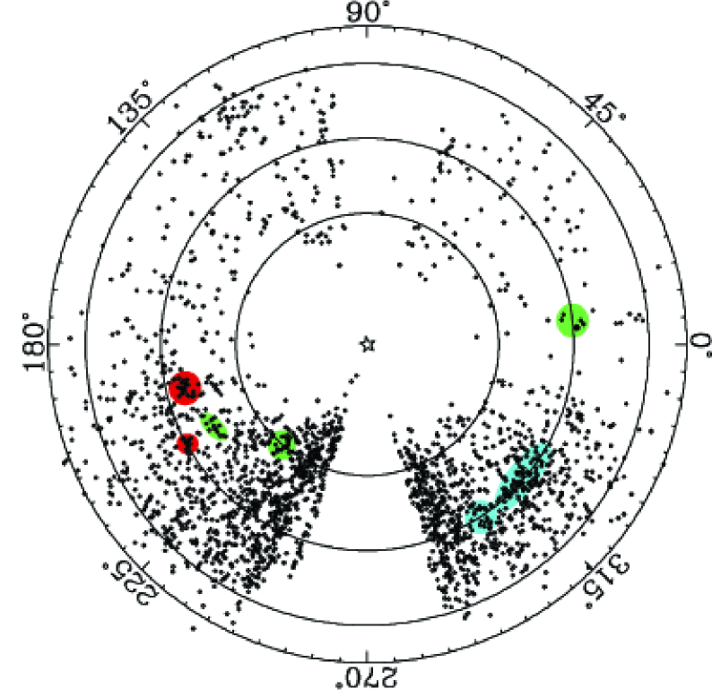
Figure 1: The radial distribution of RRL candidates from the SEKBO survey in ecliptic longitude, $\lambda$ (from KMP08). The concentric circles are at $V_{0}$=15, 17 and 19. Shaded areas represent regions of apparent overdensity which were followed up in the current study. Red ($\lambda\sim 195$${}^{\textrm{\scriptsize{o}}}$ and $210$${}^{\textrm{\scriptsize{o}}}$): VSS region; Blue ($\lambda\sim 305$${}^{\textrm{\scriptsize{o}}}$ and $315$${}^{\textrm{\scriptsize{o}}}$): Sgr region; Green ($\lambda\sim 210$${}^{\textrm{\scriptsize{o}}}$, $230$${}^{\textrm{\scriptsize{o}}}$ and $5$${}^{\textrm{\scriptsize{o}}}$): 14h, 16 h, and 0 h regions.

In addition to the 51 RRLs from the clumps which were targeted for spectroscopic follow-up, a selection of a further 55 candidates over a wide range of RAs was targeted for photometric follow-up in order to elucidate the nature of the contamination of the SEKBO RRL candidate sample by non-RRLs. These targets varied in magnitude between $V$ = 15 and 19.5. This set of targets included a selection of ‘red’ variable objects to investigate whether the adopted dereddened color cutoff of $(V-R)_{0}=0.3$ for RRL candidates was appropriate. The number of spectroscopy and photometry targets in each region is summarized in Table 1.

2.2 Photometry

Observations were made with the Australian National University (ANU) $40^{\prime\prime}$ telescope at Siding Spring Observatory (SSO) over six six-night runs between November 2006 and October 2007. The target was centered on one of the Wide Field Imager’s eight CCDs. The $V$ filter was used, with exposure times ranging from 120 to 600 s depending on the target magnitude. The total number of observations for each target over the observing runs ranged from 5 to 19, with an average of 9 observations per target (see Figure 2).

Figure 2: The distribution of number of observations for imaged candidates.

The data were overscan subtracted, trimmed, bias subtracted and flatfielded with twilight sky flats using standard IRAF procedures. Aperture photometry was then performed on each target as well as on an ensemble of nearby comparison stars, yielding an average differential magnitude for each target at each epoch. This series of differential magnitudes for the target was subsequently entered into Andrew Layden’s period-fitting routine (Layden & Sarajedini 2000 and references therein) along with the mid-exposure heliocentric Julian dates of the observations. Layden’s routine identifies the most likely period by fitting the photometry of the variable star with 10 templates (including 7 RRL templates) and performing a $\chi^{2}$ minimization. See Pritzl et al. (2002) for a more detailed description of the method. The best obtained period was then entered into Layden’s light curve-fitting routine. Example candidate light curves are displayed in Figure 3.

Figure 3: Phased $V$ mag differences between a candidate and nearby comparison stars. From the tight fit of the data points to the template light curves (solid line), we can be very confident that these two candidates are indeed RR Lyrae stars. Left: RR$ab$ with period = 0.583 d. Right: RR$c$ with period = 0.358 d.

One important application of the analysis of this photometry was to determine which candidates were indeed RRL stars and which were spurious detections. Of the 73 stars observed at least 8 times, 11 had magnitudes which did not vary significantly over the observations, 4 were classified as binary stars and 7 showed variability but did not appear to have periods and light curves corresponding to either RRLs or binary stars. Figure 4 shows the number of candidates falling into each classification category as a function of $(V-R)_{0}$.

Given that there are 51 RRLs and 16 non-RRLs within the color selection, this indicates that the procedure KMP08 used to identify RRLs from the SEKBO survey data has a contamination rate of 24 $\pm$ 7%, where the uncertainty has been calculated using Poisson statistics. Table 4 summarizes the photometric data, including the classification, period and fitted $V$ amplitudes (where applicable) for all targets.

Figure 4: The classification of RRL candidates based on follow-up photometry. The dashed line indicates the adopted color cutoff of $(V-R)_{0}<0.3$ for RRL candidates in the SEKBO survey.

2.3 Spectroscopy

Observations were made with the ANU 2.3 m telescope at SSO in runs that were concurrent with those on the $40^{\prime\prime}$ telescope. The blue arm of the Double Beam Spectrograph was used with a $2^{\prime\prime}$ slit and the 600B grating, giving a resolution of $\sim$2 Å. The spectra were centered on 4350 Å so that the Ca II K line and Hydrogen lines such as H$\delta$, H$\gamma$ and H$\beta$ could be observed. Exposure times were chosen to give a signal-to-noise of $\sim$20 and varied between 900 and 3000 s. Each target was observed between one and four times, spread throughout a given observing run. Each observation was accompanied by a comparison Cu Ar lamp exposure. Radial velocity standards of similar spectral type were also observed for use as cross-correlation templates (see §3) as well as standards for Layden’s (1994) pseudo-equivalent width system (see §4). A small number of bright RRLs from Layden (1994) were also observed to serve as additional cross-correlation templates.

The data were overscan subtracted and trimmed using standard IRAF procedures. Bias subtraction and flatfielding were not performed as they only served to add noise to the data. Wavelength calibration was performed over the range 3500–4965 Å using 4th–8th order legendre polynomials and 26–28 spectral lines, yielding dispersion solutions with RMS $\sim$ 0.05 Å. Example spectra (after continuum fitting as described in §4) are displayed in Figure 5 and demonstrate the range in quality obtained.

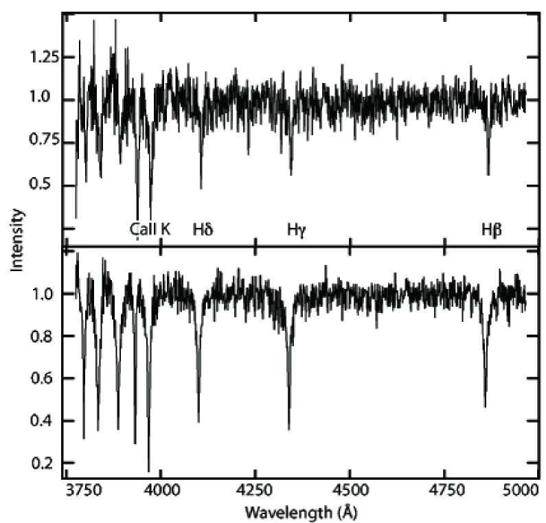
Figure 5: Examples of poor quality (top) and good quality (bottom) normalized spectra.

3 Radial Velocities

Radial velocities were determined using the IRAF task fxcor which performs Fourier cross-correlations between spectra of the target star and chosen template stars. For each observing run, we chose 5–6 stars to use as templates from amongst the radial velocity standards and the bright RRLs from Layden (1994). The selection process was guided by the fact that relative velocities between template and target stars were most precise when the two stars were of similar spectral type. Subsequently, heliocentric corrections were made to remove the component of the observed velocity due to the Earth’s motion around the Sun.

Observed radial velocities of an RR$ab$ star can vary up to $\pm$50 km s^-1 from its systemic velocity as a function of phase. In order to correct the observed velocities to systemic velocities we first determined the phase of each observation using the ephemerides based on the best period obtained from our photometric data. Layden’s (1994) parametrization of the velocity curve for the RRL star X Ari (measured by Oke (1966) from the H$\gamma$ line) was then used to determine the systemic velocity. Figure 6 shows example fits of the curve to our observed data. Based on X Ari, the systemic velocity is taken to occur at phase 0.5. Note that because the form of the discontinuity in the light curve near maximum light varies amongst RRLs, only phases between 0.1 and 0.85 were used in the fit. The average RMS of the fits was 18 km s^-1, which we use as an estimate of the uncertainty in the conversion from observed velocities to systemic velocities. We then combine this with the average uncertainty in the radial velocity zeropoints across the observing runs ($\pm 7$ km s^-1) and the uncertainty in the cross-correlations ($\pm 4$ km s^-1). The latter was quantified by calculating, for each observation, the standard deviation of the velocities obtained using the different templates, then averaging over all observations. The combination of these errors then yields an overall uncertainty in the systemic radial velocities of $\pm 20$ km s^-1. For the one RRL in common with Duffau et al. (2006), the velocities agree within the combined errors.

Figure 6: Fits of the radial velocity template of X Ari (solid line) to three type $ab$ RRLs in our sample, each observed at three phases. The upper two plots are examples of excellent fits, while the lowest plot is an example of a poor fit. Note that data points with phase $<$ 0.1 or phase $>$ 0.85 are excluded in the fit. The systemic velocity corresponds to phase 0.5.

Of the 51 spectroscopic targets, 13 were type $c$ RRLs. For these stars, velocity data for DH Peg and T Sex (Liu & Janes, 1989; Jones et al., 1988) were used to create a template velocity curve. However, given that the template yielded uncertainties in systemic velocities of up to 30 km s^-1 when fitted to our data, we opted to instead use the average radial velocity as our estimate of the systemic velocity. Taking into consideration the precision of our measurements and the fact that observed radial velocities of an RR$c$ star at different phases only vary by up to $\pm$30 km s^-1 from its systemic velocity, one would not expect a fit to a template curve to provide an improved constraint on the systemic velocity. This was indeed evidenced by the large scatter in the residuals of the template fit to the data as a function of phase. The average radial velocity was also used as an estimate of the systemic velocity for the four type $ab$ RRLs having all observations at phases less than 0.1 or greater than 0.85. This non-optimal method likely produced inflated radial velocity uncertainties for these stars.

When investigating Galactic substructures, it is useful to consider radial velocities in a frame of reference which is at rest with respect to the Galactic center. The heliocentric radial velocities ($V$${}_{\textrm{\scriptsize{helio}}}$) calculated as described above were thus transformed to Galactic standard of rest frame velocities ($V$${}_{\textrm{\scriptsize{GSR}}}$), thereby removing the effects of the Sun’s peculiar motion (assumed to be $(u,v,w)=(-9,11,6)$ km s^-1 with respect to the local standard of rest which has a rotation of 220 km s^-1). The determined radial velocities, $V$${}_{\textrm{\scriptsize{helio}}}$ and $V$${}_{\textrm{\scriptsize{GSR}}}$, for RRLs in the VSS region and the 14 h, 16 h and 0 h regions are given in Table 5.

3.1 Virgo Stellar Stream region

The spatial distribution and $V$${}_{\textrm{\scriptsize{GSR}}}$ of observed RRLs in VSS Clumps 1 and 2 are displayed in Figure 7. Distances are based on the assumption of $M_{V}$ = 0.56 and have an uncertainty of $\sim$7%, as described in KMP08. This corresponds to an uncertainty of approximately $\pm$1 kpc at a distance of 20 kpc. RRLs observed spectroscopically by Duffau et al. (2006) (hereafter DZV06) and classified as VSS members are also included on the Figure to show the region where the VSS was detected. The four magenta points have $40$ km s^-1 $<$ $V$${}_{\textrm{\scriptsize{GSR}}}$ $<160$ km s^-1, the range within which DZV06 classified RRLs as members of the VSS. One star has previously been associated with the VSS by DZV06 while the remaining three proposed members are new discoveries. They would suggest that the stream spans a much larger declination range than previously estimated. The four members have $\langle$$V$${}_{\textrm{\scriptsize{GSR}}}$$\rangle$ = $127\pm 10$ km s^-1 and dispersion $\sigma=27$ km s^-1 which is only slightly larger than the measurement error of $\pm 20$ km s^-1. Our value of $\langle$$V$${}_{\textrm{\scriptsize{GSR}}}$$\rangle$ is somewhat higher than DZV06’s value of $100\pm 8$ km s^-1 and is in better agreement with Newberg et al.’s (2007) value of $130\pm 10$ km s^-1.

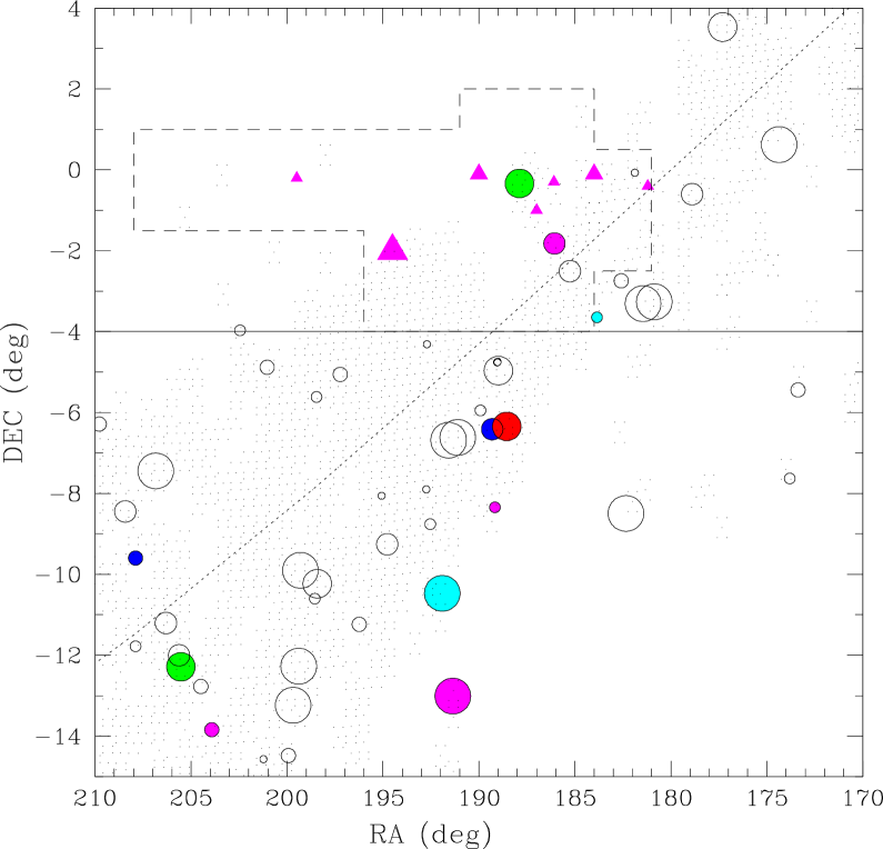
Figure 7: The spatial distribution of RRL candidates from the SEKBO survey (circles) and QUEST RRLs found to be VSS members (triangles). Symbol size represents distance, ranging from 16 kpc (largest) to 22 kpc (smallest). Filled circles were observed spectroscopically and are color-coded according to $V$${}_{\textrm{\scriptsize{GSR}}}$. Blue: less than $-160$ km s^-1; Cyan: $-160$ to $-40$ km s^-1; Green: $-40$ to 40 km s^-1; Magenta: 40 to 160 km s^-1 and Red: greater than 160 km s^-1. The dotted line is the ecliptic and the small dots represent the coverage of the SEKBO survey fields in this part of the sky. The dashed box is the region where Duffau et al. (2006) identified the VSS as an excess of main-sequence stars of appropriate apparent magnitude. The approximate southern limit of SDSS data in this region is shown by the solid line at Dec = $-4$${}^{\textrm{\scriptsize{o}}}$.

Figure 8 is a generalized histogram of $V$${}_{\textrm{\scriptsize{GSR}}}$ in which each observed value is represented by a normal distribution with mean equal to the observed value and standard deviation comparable to the uncertainty in the measurement. Summing probability density distributions over all observations then yields an estimate of the true distribution of $V$${}_{\textrm{\scriptsize{GSR}}}$ which, unlike in standard histograms, does not vary according to binning choice. A random selection of halo stars is expected to have a normal distribution of radial velocities (e.g. Harding et al. 2001) with a mean of $\sim$0 km s^-1 and a standard deviation of $\sim$100 km s^-1(e.g. Sirko et al. 2004; Brown et al. 2005) (dotted line on Figure 8). Our data does not fit the expected distribution well, though the difference did not reach statistical significance in a Kolmogorov-Smirnov test due to the small sample size.

On visual inspection, however, there is a suggestion of a peak at $\sim$130 km s^-1 (VSS members) and a second at large negative velocities. The three stars contributing to this latter peak, for which $\langle$$V$${}_{\textrm{\scriptsize{GSR}}}$$\rangle$ = $-175\pm 10$ km s^-1, are similar in velocity (and general spatial location) to the excess of stars identified by Newberg et al. (2007) at $V$${}_{\textrm{\scriptsize{GSR}}}$ $=-168\pm 10$ km s^-1 and (RA, Dec) $\approx$ (191${}^{\textrm{\scriptsize{o}}}$, $-8$${}^{\textrm{\scriptsize{o}}}$). Newberg et al. (2007) did not suggest an association for this peak, but it has the appropriate $V$${}_{\textrm{\scriptsize{GSR}}}$ to be associated with the Sgr leading tidal tail, which is expected to have a highly negative radial velocity at this RA (e.g. see modeling by Law et al. 2005). However, debate currently surrounds the question of whether Sgr debris, coming from the north Galactic pole to the solar neighborhood, is in fact densely located in this region (Martínez-Delgado et al., 2007; Newberg et al., 2007). Newberg et al. do concede, however, that the VSS and Sgr streams overlap, so while it is not expected to be dense enough in this region to account for the entire overdensity in Virgo, it seems plausible that a portion could be attributed to Sgr leading debris.

Figure 8: Generalized histogram of $V$${}_{\textrm{\scriptsize{GSR}}}$ (with kernel of 20 km s^-1) for the eleven observed RRLs in the VSS region (left) and for the fourteen RRLs in the 14 h, 16 h, and 0 h regions (right). Overplotted (dotted line) is the expected distribution of $V$${}_{\textrm{\scriptsize{GSR}}}$ given a halo population in which velocities are normally distributed with $\langle$$V$${}_{\textrm{\scriptsize{GSR}}}$$\rangle$ = 0 km s^-1 and $\sigma$ = 100 km s^-1. The VSS can be seen in the left panel as the excess of stars at $V$${}_{\textrm{\scriptsize{GSR}}}$ $\sim 130$ km s^-1, while the excess at $V$${}_{\textrm{\scriptsize{GSR}}}$ $\sim-170$ km s^-1 could potentially be related to leading Sgr debris.

3.2 Regions at RA 14 h, 16 h, and 0 h

No groupings of velocities were noted in the apparent spatial clumps at 14 h, 16 h, and 0 h, though it should be noted that the small sample sizes might have made any moving groups difficult to detect. We note, however, that the $V$${}_{\textrm{\scriptsize{GSR}}}$ distribution of RRLs in these regions (see the right panel of Figure 8) more closely resembles the expected normal distribution of halo stars than does the distribution of RRLs in the VSS region. As mentioned above, the 20 and 21.5 h regions overlap with the Sgr trailing debris stream and the results will be discussed in a separate paper.

4 Metal Abundances

Metallicities ([Fe/H]) were calculated using the Freeman & Rodgers (1975) method which is an analogue of Preston’s (1959) classic $\Delta$S technique. In the Freeman & Rodgers method, metal abundance is determined by plotting the pseudo-equivalent width (EW) of the Ca II K line, $W$(K), against the mean EW of the Balmer lines, $W$(H). As the RRL varies in phase, it traces out a path on this plot which is strongly dependent on its metallicity. Thus, by using a calibration based on RRLs of known metallicity, we can determine [Fe/H] for our sample from low resolution spectra. Note that observations taken during rising light (phase $\sim$ 0.8–1) should not be used since changes in the RRL’s effective gravity and Balmer line profiles during this stage alter the relationship between $W$(K) and $W$(H). We have also omitted type $c$ RRLs from the metallicity analysis since they are hotter and have weaker Ca II K lines than type $ab$ RRLs. Lower signal-to-noise spectra and uncertainties in the contamination from interstellar Ca II K would thus result in larger uncertainties in the metallicities of type $c$ RRLs compared to type $ab$.

The first step was to normalize our wavelength-calibrated spectra to unit intensity using IRAF’s continuum task, which divides each spectrum by an appropriate polynomial. Subsequent steps closely followed the method described in Layden (1994). Eight of Layden’s EW standard RRLs had been observed multiple times over the course of our observing runs. $W$(K) (corrected for interstellar contamination using the Beers 1990 model) and the EWs of the Balmer lines H$\delta$, H$\gamma$ and H$\beta$ were measured using numerical integration, with feature bands and continuum bands equal to Layden’s wherever possible (see Table 2). Unlike Layden, however, the $W$(K) continuum bands were fixed for all reductions and our red continuum band for H$\beta$ was truncated due to our smaller wavelength coverage. Also note that all bands were offset by an appropriate wavelength shift according to the observed geocentric radial velocity of each spectrum (described in §3).

The measured equivalent widths for the standard RRLs are shown in Table 3 and offsets from Layden’s values are displayed in Figure 9. It can be seen that our values agree well with Layden’s for $W$(K), $W$(H$\delta$) and $W$(H$\gamma$) but that our values for $W$(H$\beta$) are systematically smaller than Layden’s. This was likely due to the use of a different red continuum band as mentioned above. A linear regression was performed to calculate the appropriate correction to bring our $W$(H$\beta$) measurements in line with Layden’s. The best fit is overplotted on Figure 9.

Figure 9: Differences between pseudo-equivalent widths (top to bottom: $W$(K), $W$(H$\gamma$), $W$(H$\delta$), $W$(H$\beta$)) in the current study and those of Layden (1994) for eight EW standard stars. Negative $\Delta W$ values indicate that our EWs are smaller than those of Layden. Error bars are the standard deviations of our repeated measures of the EWs (see Table 3 for details). No appreciable difference was noted for $W$(K), $W$(H$\gamma$) or $W$(H$\delta$) (horizontal line drawn at $\Delta W$ = 0 for reference) but a negative linear relationship was noted for $W$(H$\beta$), as shown by the solid line in the lowest plot.

Figure 10: The pseudo-equivalent width of the Ca II K line, corrected for interstellar absorption, against the average width of H$\delta$, H$\gamma$ and H$\beta$ for the 16 type $ab$ RRLs in the 14 h, 16 h, 0 h and VSS regions. Solid lines connect values for the same RRL observed at different phases. The dashed lines are the loci of stars having the indicated [Fe/H] value according to Layden’s (1994) calibration. The two hypothesized VSS members are plotted as open squares.

With the offsets to Layden’s system in hand, the process of normalization and measurement of EWs was repeated for the target RRLs. In Figure 10, $W$(K), corrected for interstellar Ca II K, is plotted against $W$(H3), the average of the EWs of H$\delta$, H$\gamma$ and H$\beta$ (offset to Layden’s system). The dashed lines are given by

$$W a bW c dW$$(K) = + (H) + [Fe/H] + (H)[Fe/H],

using coefficients determined by Layden (1994) that yield an external precision for [Fe/H] of $0.15$–$0.20$ dex. The values of [Fe/H] determined from this equation for the 16 type $ab$ RRLs are listed in Table 5 and their distribution is shown in Figure 11. Where more than one observation exists, the tabulated values were calculated by averaging the [Fe/H] values from the different phases (cf.  Figure 10). Based on the stars with multiple observations, the internal precision of a single [Fe/H] determination is 0.20 dex. For this sample $\langle$[Fe/H]$\rangle$$=-1.86\pm 0.1$ with a dispersion $\sigma$ = 0.45 dex (see Figure 11). This value is somewhat more metal poor than that, $\langle$[Fe/H]$\rangle$$=-1.61\pm 0.06$, $\sigma$ = 0.4 dex, tabulated by Kinman et al. (2000) for RRLs in the halo. The two proposed VSS members (the other two members are type $c$ RRLs for which metallicities could not be calculated) have $\langle$[Fe/H]$\rangle$$=-1.95\pm 0.1$ on our [Fe/H] system and an abundance range of $0.4\pm 0.2$ dex. These values agree with $\langle$[Fe/H]$\rangle$${}_{\textrm{\scriptsize{VSS}}}$ $=-1.86\pm 0.08$, $\sigma$ = 0.40 dex found by DZV06, supporting our claim that these stars are part of the stream. The two type $ab$ RRLs in the negative $V$${}_{\textrm{\scriptsize{GSR}}}$ peak in Figure 8, which may be associated with Sgr debris, have $\langle$[Fe/H]$\rangle$$=-1.57\pm 0.1$ and an abundance range of $0.2\pm 0.1$ dex.

Figure 11: Generalized histogram of [Fe/H] (with kernel of 0.1 dex) for the 16 type $ab$ RRLs in the 14 h, 16 h, 0 h, and VSS regions.

5 Luminosity Functions

Having discovered three RRLs with radial velocities and metal abundances consistent with the VSS yet falling outside the VSS region identified by DZV06, it was of interest to further explore the spatial extent of the stream by now examining a broader stellar population. We selected 49 2${}^{\textrm{\scriptsize{o}}}$$\times$2${}^{\textrm{\scriptsize{o}}}$ regions spread over RA 125–220${}^{\textrm{\scriptsize{o}}}$ with the aim of sampling the area roughly evenly, given the constraints of the actual SEKBO field locations (see Figure 12). Color-magnitude diagrams (CMDs) and luminosity functions (LFs) were constructed from the SEKBO data (examples are shown in Figure 13) and examined for signs of an upturn near the magnitude where the subgiant branch and the main sequence merge. For an old population, this occurs at $M_{V}\approx 3.5$ which corresponds to $V\approx 19.9$ at a distance of 19 kpc (the average distance of the four identified VSS members, consistent with the findings of Newberg et al. 2002 and DZV06). This technique was also used by DZV06, where the target region was compared to a control region of equal area. Given the difficulty in identifying a suitable control region when the spatial extent of the VSS is unclear, we opted instead to compare the observational data to synthetic data produced by the Besançon model of Galactic stellar populations (Robin et al., 2003). This model comprises four components: thin disk, thick disk, halo and bulge. It is a smooth, dynamically self-consistent model where parameters are forced to follow physical laws, taking into account physical links between density, velocity and metallicity distribution.

The simulations covered a distance interval of 0–120 kpc and assumed an average interstellar extinction coefficient of $A_{V}$ = 0.75 mag kpc${}^{\textrm{\scriptsize{-1}}}$. This value was chosen so that the average integrated line-of-sight extinction was in agreement with those derived using the dust maps of Schlegel et al. (1998) and it is close to the value suggested by Robin et al. (2003) for intermediate to high galactic latitudes (the region studied here covers $30^{\textrm{\scriptsize{o}}}\lesssim b\lesssim 60^{\textrm{\scriptsize{o}}}$). Initial cuts in magnitude ($13<V<22$) and color ($-0.5<V-R<1.5$) were made. In order to omit local red dwarfs and focus more clearly on the population of interest, only stars with $(V-R)_{0}<0.7$ were included in the luminosity functions. Since the simulated color interval greatly exceeded the observational color errors, the simulations were not convolved with photometric errors. Similarly, completeness of the observations was not incorporated into the simulated data since our analyses would focus on stars brighter than the observational incompleteness limit.

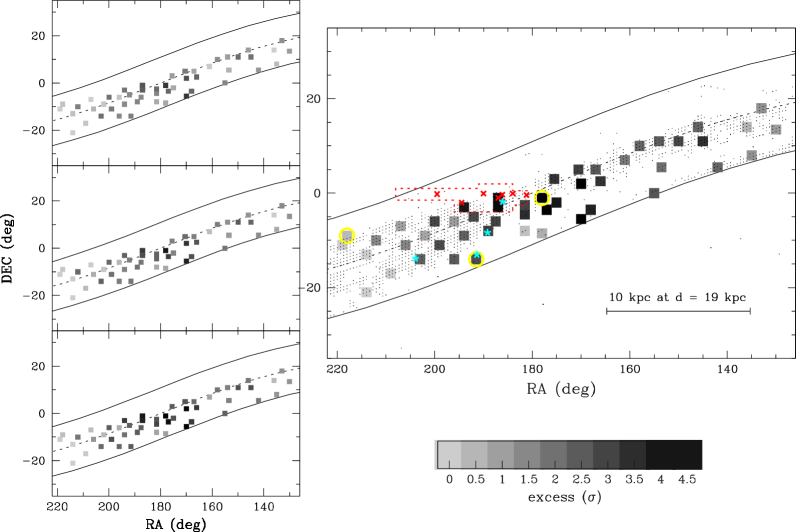
Figure 12: The spatial distribution of regions in which data was compared to the Galactic stellar distribution model. The significance of the excess of data stars over synthetic stars is represented by the coloring of the region according to the scale shown, with darker shades indicating a more significant excess. The range of magnitudes included in the excess calculation was $V_{0}$ = 16.25 to (left panel, top to bottom) 18.25, 18.75, 19.25 or (right panel) 19.75. Also shown are the four stars from our sample with $V$${}_{\textrm{\scriptsize{GSR}}}$ consistent with the VSS (cyan asterisks) and those found by DZV06 in QUEST data (red crosses). The example regions in Figure 13 are circled in yellow. As in Figure 7, the red dashed box is DZV06’s identification of the VSS region. The dashed line represents the ecliptic and the solid lines outline the broad limits of the SEKBO survey, with small dots showing the centers of the fields surveyed.

Equatorial coordinates of the regions simulated were identical to those of the chosen observed regions (with a step size of 1${}^{\textrm{\scriptsize{o}}}$ in both RA and Dec), however, areas were not equal due to the non-uniform sampling of the SEKBO survey (see the small dots in the righthand panel of Figure 12). In order to compare the LFs, we thus normalized the synthetic data to the observed data based on counts in the range $14.7<V_{0}<16$. As an example, Figure 13 shows CMDs and LFs for three regions. In the upper panel, a clear excess of observed stars over synthetic stars can be seen for $V_{0}>16.5$, peaking at $V_{0}\sim 19.5$. It should be noted that incompleteness becomes a significant factor by $V=19$ and thus the excess may well continue to grow to fainter magnitudes. In this particular region, two excesses are apparent in the CMD for stars fainter than $V\sim 19$. One has $(V-R)_{0}\sim 0.35$ while the other is redder, with $(V-R)_{0}\sim 0.6$. These excesses possibly correspond to the top of the main sequence and the lower giant branch, respectively. We verified that the excess in the luminosity function is still present using a bluer cutoff, $(V-R)_{0}<0.5$, and thus the excess is not driven solely by the redder stars. In the middle panel, the overall excess is smaller, becoming noticeable only at $V_{0}\sim 17.5$ and apparently peaking at $V_{0}\sim 19$ before incompleteness sets in. There is thus some evidence for the VSS in the region represented in the middle panel and evidence for a strong signal in the region represented in the top panel. The data in the bottom panel follows the synthetic data closely, until dropping off at the faint end when incompleteness sets in. Such regions show no evidence of the presence of the VSS.

As confirmation of these results, for those regions north of the declination limit of the SDSS we carried out a similar comparison using SDSS data rather than that from the SEKBO survey. The SDSS data have the advantage of deeper limiting magnitude and complete area coverage. In Figure 14 we show comparisons similar to those of Figure 13, but with the predictions of the Besançon model now compared to SDSS data, again for 2${}^{\textrm{\scriptsize{o}}}$$\times$2${}^{\textrm{\scriptsize{o}}}$ regions. As for the SEKBO data, the color-magnitude diagrams and luminosity functions in Figure 14 exclude local red dwarfs by considering only stars with $(g-r)_{0}<1.0$, equivalent to $(V-R)_{0}\approx 0.7$. The upper panels of Figure 14 are in fact for the same region as the upper panels of Figure 13, and, comfortingly, the results are very similar. There is an increasing excess of stars above the model predictions with decreasing magnitude that continues beyond the completeness limit of the SEKBO data, confirming that the VSS is strongly present in this region. The other two panels show different regions to those in Figure 13, though they were selected in a similar way: the middle panel is for the region centered on (RA, Dec) = (170${}^{\textrm{\scriptsize{o}}}$, +2${}^{\textrm{\scriptsize{o}}}$) where the SEKBO data predicts the VSS is present (cf. Figure 12) and the lower panel is for the region (135${}^{\textrm{\scriptsize{o}}}$, +8${}^{\textrm{\scriptsize{o}}}$) where no significant excess is predicted. In both instances the comparison with the SDSS data confirms the interpretation of the SEKBO data.

Figure 13: Left panels: Example CMDs from observed data for 2${}^{\textrm{\scriptsize{o}}}$$\times$2${}^{\textrm{\scriptsize{o}}}$ (non-uniformly sampled) regions (see yellow circles on Figure 12 for spatial locations). Middle panels: Corresponding CMDs from synthetic data using the Bescançon model (Robin et al., 2003), not convolved with completeness or photometric errors. Note that the areas have not been normalized in constructing the CMDs. Right panels: Luminosity functions for observed (solid line) and synthetic data (normalized over $14.7<V_{0}<16$; dashed line) in each region for stars with $(V-R)_{0}<0.7$. Poisson error bars are shown. The field in the top panel (RA $\sim 178$${}^{\textrm{\scriptsize{o}}}$) shows a large excess of stars in the data compared to the model, providing strong evidence for the presence of the VSS. The field in the middle panel (RA $\sim 192$${}^{\textrm{\scriptsize{o}}}$) shows a weaker excess, while the field in the bottom panel (RA $\sim 218$${}^{\textrm{\scriptsize{o}}}$) shows no excess.

Figure 14: Color-magnitude diagram and luminosity function comparisons as for Figure 13 but now with SDSS observational data rather than SEKBO data. The field for the upper panels is the same as in Figure 13. Left panels: CMDs for 2${}^{\textrm{\scriptsize{o}}}$$\times$2${}^{\textrm{\scriptsize{o}}}$ regions from the SDSS. Right panels: Luminosity functions for observed (solid line) and synthetic data (normalized over $14.9<g_{0}<16.2$; dashed line) in each region for stars with $(g-r)_{0}<1.0$. Poisson error bars are shown. As in Figure 13 the top panel shows a large excess of stars compared to the model, providing strong evidence for the presence of the VSS. The field in the middle panel (170${}^{\textrm{\scriptsize{o}}}$, +2${}^{\textrm{\scriptsize{o}}}$) also shows an excess, while the field in the bottom panel (135${}^{\textrm{\scriptsize{o}}}$, +8${}^{\textrm{\scriptsize{o}}}$) shows reasonable agreement between the model and the observations. These are consistent with the SEKBO data for these fields (cf. Figure 12).

With this confirmation of the utility of the SEKBO data, we now examine the excess quantitatively, by computing for each region the average difference between the observed data counts and the normalized model counts between $V_{0}=16.25$ and $V_{0}=$18.25, 18.75, 19.25 or 19.75. Differences were calculated in 0.5 mag bins and divided by the error in the difference, taken as the combined Poisson error in the data and normalized model counts. The average error-weighted difference over the magnitude bins was then taken as a measure of the significance of the excess in each region. Figure 12 displays the significance of the excess, represented by the grayscale shading, as a function of spatial position. The regions colored black have a 4.5$\sigma$ excess of data stars over model stars, providing strong evidence for the presence of the VSS in those regions. Since the excess appears to peak at $V_{0}\sim 19.5$ or fainter, it is not surprising that using 19.75 as the faint limit of the excess calculation (right panel) provides the highest sensitivity to detection of the VSS. The VSS signal is, however, present at brighter magnitudes, albeit more weakly (left panels). Taking into account the scarcity of sampled fields to the west of RA $\sim 180^{\textrm{\scriptsize{o}}}$, the overall pattern of excess significance is not inconsistent with the location of overdensities (Clumps 1 and 2) of the SEKBO survey RRL candidates at this distance.

While the foregoing analysis provided a significance map of the VSS, it is also desirable to construct a density map so that the absolute magnitude of the entire stream can be estimated. To do this, we scaled both observed and synthetic counts by the actual area covered. After normalizing the synthetic data to the observed data based on counts between $14.7<V_{0}<16.0$ and subtracting synthetic data from observed data, we then had a measure of the excess number of stars per square degree in each 0.5 mag bin between $V_{0}=16.25$ and 19.75. This excess number, summed over magnitude, is represented by the grayscale shading in Figure 15, with black indicating a 500 star excess per square degree. The overall pattern of excess is similar to the significance map in the righthand panel of Figure 12, with perhaps the southern regions showing a stronger signal in the density map than in the significance map. This could be understood in terms of the relative significance of the feature decreasing towards the Galactic plane due to the increase in background Milky Way stars, while the number density of stars in the feature in fact remains constant.

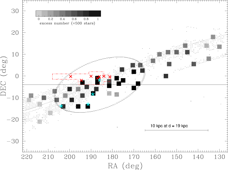
Figure 15: The spatial distribution of regions in which data was compared to the Galactic stellar distribution model. The number of excess data stars over synthetic stars is represented by the coloring of the region according to the scale shown, with darker shades indicating a larger excess. The range of magnitudes included in the excess calculation was $16.25<V_{0}<19.75$. Also shown are the four stars from our sample with $V$${}_{\textrm{\scriptsize{GSR}}}$ consistent with the VSS (cyan asterisks) and those found by DZV06 (red crosses). The ellipse outlines the estimated area of the VSS based on the current analysis. As in Figure 7, the red dashed box is DZV06’s identification of the VSS region. The dashed line represents the ecliptic and the small dots show the centres of the fields surveyed. The approximate southern limit of the SDSS coverage in this region is shown by the solid line at Dec = $-4$${}^{\textrm{\scriptsize{o}}}$.

In order to make a rough estimation of the sky coverage of the VSS, an ellipse has been overplotted on Figure 15. The chosen shape is somewhat arbitrary, with the positioning and size selected so as to include the regions in which the excess appears visually to be significant. The ellipse encompasses areas not sampled by the SEKBO survey on the basis that the VSS could plausibly extend to those areas given the distribution of high excess regions in the sampled areas and assuming a certain degree of uniformity. This assumption could lead to an overestimate in the area, but conversely, the VSS may well extend beyond the survey region (particularly to the south where no data has been gathered by previous surveys) leading to an area underestimate. Entire coverage will be possible with SkyMapper (Keller et al., 2007), but in the meantime we note that the current area estimate is likely to be uncertain by at least a factor of two.

Assuming a heliocentric distance of 19 kpc, the stream’s projection on the sky extends $\sim$15 kpc in length along the largest dimension and covers an area of $\sim$760 deg${}^{\textrm{\scriptsize{2}}}$, centered at (RA, Dec) $\sim(186^{\textrm{\scriptsize{o}}},-4^{\textrm{\scriptsize{o}}})$. This estimate of the area, with its large uncertainty, is in rough agreement with Jurić et al.’s (2008) estimate of 1000 deg${}^{\textrm{\scriptsize{2}}}$ for the VSS based on SDSS data. Not only is there evidence that the feature is much larger than DZV06’s estimate of 106 deg${}^{\textrm{\scriptsize{2}}}$ (dashed box on Figure 12), but given the non-overlapping regions of the SDSS and SEKBO survey data, the true size of the stream may well be greater than 1000 deg${}^{\textrm{\scriptsize{2}}}$. Our analysis shows the VSS to extend to the west and to the south of DZV06’s detection. We indeed found three RRLs in the southern direction with radial velocities consistent with the VSS. Note that neither QUEST nor SDSS covered Galactic latitudes lower than $\sim$60${}^{\textrm{\scriptsize{o}}}$ in this region, hence our findings provide the first tracing of this section of the stream, extending the location of the VSS well south of the declination limits of these two surveys. Jurić et al. (2008) found that the number density of stars belonging to the feature increases towards the Galactic plane and indeed we find that the VSS extends to at least $b\sim 45^{\textrm{\scriptsize{o}}}$ (Dec $\sim-15$${}^{\textrm{\scriptsize{o}}}$).

Having estimated the area of the VSS, it is now possible to calculate an estimate of the absolute magnitude, $M_{V}$, of the stream. The fluxes for the excess stars in each magnitude bin ($16.25<V_{0}<19.75$) were averaged over all the regions contained within the ellipse, summed over the magnitude bins and finally, multiplied by the area of the ellipse. Assuming a distance of 19 kpc and an area of 760 deg${}^{\textrm{\scriptsize{2}}}$ and using $V$ band values of $M_{\odot}=4.83$ and $L_{\odot}=4.64\times 10^{25}$ W (Binney & Merrifield, 1998), we calculate $M_{V}=-11.9$ mag. This value is considerably brighter than $M_{R}=-8.0$ mag estimated by Jurić et al. (2008). We note, however, that their value assumed a distance of 10 kpc, an area of 1000 deg${}^{\textrm{\scriptsize{2}}}$ and magnitude limits of $18<R<21.5$. Using values as close to these as possible given the constraints of our data, our estimate becomes $M_{V}=-10.1$ mag.

A final point to note is that Jurić et al. (2008) find the VSS to span $\sim$10 kpc along the line-of-sight, at distances closer than where it was detected by the SEKBO survey, and that their survey data did not go beyond a scale height of $Z=20$ kpc. It thus seems a likely scenario that the VSS spans many kpc along the line-of-sight (indeed DZV06 found possible members at distances ranging between 16 and 24 kpc and new results of Vivas et al. 2008 find possible members as close as 12 kpc) but is more diffuse at distances $\lesssim$15 kpc, with the highest concentration at $d\sim 19$ kpc. Considering that Jurić et al. (2008) do not include the portion at $d\sim 19$ kpc in their $M_{R}$ calculation, it is not surprising that their value should be considerably fainter than ours. It is also important to note that all our values are lower limits only, since stars brighter than $V_{0}=16.25$ and fainter than $V_{0}=19.75$ were not included. In addition, incompleteness was not taken into account. The estimate is also sensitive to the area covered, distribution of VSS density within that area and to the distance of the stream, each of which are somewhat uncertain based on the sampling of the data currently available and the likely extended nature of the stream along the line-of-sight.

Nevertheless, the VSS is clearly a significant local structure. Its origin remains unclear, though the large abundance range observed ($\sim$0.4 dex) is consistent with DZV06’s suggestion that the VSS is the disrupted remnants of a dwarf Spheroidal galaxy. It is certainly a large, diffuse structure and is likely to have a substantial total luminosity. Future kinematic observations are needed to further constrain the properties of the system and to provide additional clues to its origin.

6 Conclusions

Analysis of follow-up spectroscopy of eleven photometrically confirmed RRLs from a candidate list based on SEKBO survey data has revealed three new RRLs with velocities consistent with membership in the Virgo Stellar Stream, in addition to one previously identified member ($\langle$$V$${}_{\textrm{\scriptsize{GSR}}}$$\rangle$= $127\pm 10$ km s^-1, $\sigma=27$ km s^-1). The two type $ab$ members have $\langle$[Fe/H]$\rangle$ = $-1.95\pm 0.1$ and an abundance range of $\sim$0.4 dex, consistent with values found by DZV06 for the VSS. The newly discovered VSS members occupy a region of space covered by neither QUEST nor SDSS data, to the south-east of the apparent center of the stream at (RA, Dec) $\sim$ ($186^{\textrm{\scriptsize{o}}},-4^{\textrm{\scriptsize{o}}}$). Comparison of luminosity functions for observed data compared to data synthesized with the Besançon Galactic model (Robin et al., 2003) revealed the VSS to be a large, diffuse feature, covering at least 760 deg² of sky. The core of the VSS appears to have an angular size of $\sim$45${}^{\textrm{\scriptsize{o}}}$ along the longest dimension, corresponding to a spatial scale of $\sim$15 kpc in projection, assuming a heliocentric distance of $\sim$19 kpc. We have traced the stream as far south as Dec $\sim-14$${}^{\textrm{\scriptsize{o}}}$ and to Galactic latitudes as low as $b\sim 45$${}^{\textrm{\scriptsize{o}}}$.

Table 1: Target Summary

	Number of Targets
Photometry and Spectroscopy
VSS:
stringClump 1 (12.4 h)	8
stringClump 2 (14 h)	3
Sgr:
stringClump 1 (20 h)	5
stringClump 2 (21.5 h)	21
Other clumps:
string14 h	3
string16 h	6
string0 h	5
Spectroscopy Total	51
Photometry Only
Contamination check:
string0 – 21.5 h	55
Photometry Total	106

Table 2: Feature and continuum band wavelengths (in Å)

Feature	$\lambda$${}_{\textrm{\scriptsize{feature}}}$	Feature Band		Blue Contin. Band		Red Contin. Band
		$\lambda$${}_{\textrm{\scriptsize{blue}}}$	$\lambda$${}_{\textrm{\scriptsize{red}}}$	$\lambda$${}_{\textrm{\scriptsize{blue}}}$	$\lambda$${}_{\textrm{\scriptsize{red}}}$	$\lambda$${}_{\textrm{\scriptsize{blue}}}$	$\lambda$${}_{\textrm{\scriptsize{red}}}$
Ca II K-narrow	3933.666	3927.	3941.	3908.	3923.	4019.	4031.
Ca II K-wide	3933.666	3924.	3944.	3908.	3923.	4019.	4031.
H$\delta$	4101.735	4092.	4112.	4008.	4060.	4140.	4215.
H$\gamma$	4340.465	4330.	4350.	4206.	4269.	4403.	4476.
H$\beta$	4861.327	4851.	4871.	4719.	4799.	4925.	4950.

Table 3: Standard equivalent widths (in Å)

Star	N${}_{\textrm{\scriptsize{obs}}}$	$W$(K)		$W$(H$\delta$)		$W$(H$\gamma$)		$W$(H$\beta$)
		mean	sd	mean	sd	mean	sd	mean	sd
BD-17 484	8	5.05${}^{\textrm{\scriptsize{w}}}$	0.09	3.70	0.05	3.51	0.07	3.41	0.07
HD 22413	10	3.69${}^{\textrm{\scriptsize{n}}}$	0.05	6.75	0.05	6.43	0.05	5.86	0.06
HD 65925	2	6.66${}^{\textrm{\scriptsize{w}}}$	0.04	5.33	0.06	5.08	0.07	5.04	0.01
HD 74000	4	3.31${}^{\textrm{\scriptsize{n}}}$	0.10	3.89	0.02	3.66	0.06	3.43	0.17
HD 74438	2	3.39${}^{\textrm{\scriptsize{n}}}$	0.00	8.88	0.01	8.59	0.08	7.82	0.01
HD 76483	7	2.55${}^{\textrm{\scriptsize{n}}}$	0.11	9.85	0.13	9.55	0.17	8.68	0.22
HD 78791	2	9.69${}^{\textrm{\scriptsize{w}}}$	0.03	2.47	0.07	2.48	0.06	3.79	0.07
HD 180482	4	2.57${}^{\textrm{\scriptsize{n}}}$	0.02	10.02	0.07	9.64	0.07	8.82	0.10
mean standard deviation			0.06		0.06		0.08		0.09

Note. — When $W$(K${}_{\textrm{\scriptsize{wide}}}$) $<4.0$ Å, the narrow (n) feature band was used; when $W$(K${}_{\textrm{\scriptsize{wide}}}$) $\geqslant$ 4.0 Å, the wide (w) feature band was used.

Table 4: Photometric data summary

ID	$\alpha$ (J2000.0)	$\delta$ (J2000.0)	$\langle$$V$$\rangle$	$\langle$$R$$\rangle$	$\langle$$V-R$$\rangle$0	n${}_{\textrm{\scriptsize{obs}}}$	Classification	Period (days)	$V$ Amplitude
96102-170	12 24 15.67	$-$01 49 14.52	17.02	16.83	0.174	15	RR$ab$	0.525	0.286
96637-458	08 48 02.53	17 02 45.92	17.19	16.68	0.499	6	non-variable	-	-
97883-402	13 51 34.58	$-$11 46 40.63	17.30	17.06	0.199	5	RR$ab$	0.542	0.718
97890-199	13 43 04.44	$-$11 34 05.74	16.34	16.18	0.130	6	RR$c$	0.350	0.374
97890-1542	13 45 14.61	$-$11 12 09.57	17.24	17.09	0.105	7	unclassified variable	-	-
99747-73	21 14 09.39	$-$17 36 32.90	17.09	16.91	0.135	8	RR$ab$	0.517	0.724
99752-96	21 33 35.19	$-$16 07 05.52	17.08	16.93	0.098	15	RR$c$	0.324	0.466

Note. — Table 4 is published in its entirety in the electronic version of the Journal. A portion is shown here for guidance regarding its form and content. Units of right ascension are hours, minutes, and seconds, and units of declination are degrees, arcminutes, and arcseconds.

Table 5: Spectroscopic data summary

ID	RRL	systemic vel.	n${}_{\textrm{\scriptsize{vel}}}$	$V$${}_{\textrm{\scriptsize{helio}}}$	$V$${}_{\textrm{\scriptsize{GSR}}}$	n${}_{\textrm{\scriptsize{Fe/H}}}$	[Fe/H]
	type	calculation		(km s-1)	(km s-1)
VSS region
96102-170*	$ab$	fit	2	$230$	$128$	3	$-2.15$
105648-222	$ab$	fit	1	$-91$	$-162$	1	$-1.45$
107552-323	$ab$	fit	3	$302$	$193$	3	$-1.34$
108227-529	$c$	average	1	$-8$	$-119$	-	-
109247-528	$c$	average	2	$113$	$28$	-	-
119827-670	$ab$	fit	2	$-84$	$-192$	2	$-1.68$
120185-77	$ab$	fit	2	$94$	$1$	2	$-2.38$
120679-336*	$ab$	fit	3	$204$	$91$	2	$-1.74$
120698-392*	$c$	average	1	$227$	$134$	-	-
121242-188*	$c$	average	3	$276$	$155$	-	-
121194-205	$c$	average	1	$-39$	$-152$	-	-
14 h, 16 h, and 0 h regions
97890-199	$c$	average	2	$367$	$285$	-	-
106586-211	$ab$	fit	2	$-5$	$-33$	2	$-1.52$
114421-242	$ab$	fit	1	$-51$	$40$	1	$-2.30$
120857-475	$ab$	fit	1	$191$	$100$	1	$-2.24$
121817-2385	$ab$	fit	2	$3$	$-33$	1	$-1.87$
121906-2336	$c$	average	2	$40$	$-2$	-	-
122112-595	$ab$	fit	1	$-134$	$-168$	1	$-1.42$
122156-1114	$c$	average	2	$-42$	$-81$	-	-
122214-1315	$ab$	fit	1	$24$	$-14$	2	$-1.96$
122240-33	$ab$	average	2	$121$	$21$	1	$-2.01$
127008-210	$ab$	fit	2	$-3$	$78$	2	$-0.96$
127806-85	$ab$	fit	1	$-187$	$-102$	1	$-2.63$
127806-438	$c$	average	3	$-165$	$-80$	-	-
128416-544	$ab$	fit	2	$-309$	$-192$	2	$-2.19$

Note. — Proposed VSS members are marked by *

References

- Beers (1990) Beers, T. C. 1990, AJ, 99, 323
- Bell et al. (2008) Bell, E. F., Zucker, D. B., Belokurov, V., Sharma, S., Johnston, K. V., Bullock, J. S., Hogg, D. W., Jahnke, K., de Jong, J. T. A., Beers, T. C., Evans, N. W., Grebel, E. K., Ivezić, Ž., Koposov, S. E., Rix, H.-W., Schneider, D. P., Steinmetz, M., & Zolotov, A. 2008, ApJ, 680, 295
- Belokurov et al. (2007) Belokurov, V., Evans, N. W., Bell, E. F., Irwin, M. J., Hewett, P. C., Koposov, S., Rockosi, C. M., Gilmore, G., Zucker, D. B., Fellhauer, M., Wilkinson, M. I., Bramich, D. M., Vidrih, S., Rix, H.-W., Beers, T. C., Schneider, D. P., Barentine, J. C., Brewington, H., Brinkmann, J., Harvanek, M., Krzesinski, J., Long, D., Pan, K., Snedden, S. A., Malanushenko, O., & Malanushenko, V. 2007, ApJ, 657, L89
- Belokurov et al. (2006) Belokurov, V., Zucker, D. B., Evans, N. W., Gilmore, G., Vidrih, S., Bramich, D. M., Newberg, H. J., Wyse, R. F. G., Irwin, M. J., Fellhauer, M., Hewett, P. C., Walton, N. A., Wilkinson, M. I., Cole, N., Yanny, B., Rockosi, C. M., Beers, T. C., Bell, E. F., Brinkmann, J., Ivezić, Ž., & Lupton, R. 2006, ApJ, 642, L137
- Binney & Merrifield (1998) Binney, J. & Merrifield, M. 1998, Galactic Astronomy (Princeton: Princeton Univ. Press)
- Brown et al. (2005) Brown, W. R., Geller, M. J., Kenyon, S. J., Kurtz, M. J., Allende Prieto, C., Beers, T. C., & Wilhelm, R. 2005, AJ, 130, 1097
- Carollo et al. (2007) Carollo, D., Beers, T. C., Lee, Y. S., Chiba, M., Norris, J. E., Wilhelm, R., Sivarani, T., Marsteller, B., Munn, J. A., Bailer-Jones, C. A. L., Fiorentin, P. R., & York, D. G. 2007, Nature, 450, 1020
- Chiba & Beers (2001) Chiba, M. & Beers, T. C. 2001, ApJ, 549, 325
- Duffau et al. (2006) Duffau, S., Zinn, R., Vivas, A. K., Carraro, G., Méndez, R. A., Winnick, R., & Gallart, C. 2006, ApJ, 636, L97
- Eggen et al. (1962) Eggen, O. J., Lynden-Bell, D., & Sandage, A. R. 1962, ApJ, 136, 748
- Freeman & Rodgers (1975) Freeman, K. C. & Rodgers, A. W. 1975, ApJ, 201, L71+
- Harding et al. (2001) Harding, P., Morrison, H. L., Olszewski, E. W., Arabadjis, J., Mateo, M., Dohm-Palmer, R. C., Freeman, K. C., & Norris, J. E. 2001, AJ, 122, 1397
- Ibata et al. (1994) Ibata, R. A., Gilmore, G., & Irwin, M. J. 1994, Nature, 370, 194
- Ibata et al. (2003) Ibata, R. A., Irwin, M. J., Lewis, G. F., Ferguson, A. M. N., & Tanvir, N. 2003, MNRAS, 340, L21
- Jones et al. (1988) Jones, R. V., Carney, B. W., & Latham, D. W. 1988, ApJ, 326, 312
- Jurić et al. (2008) Jurić, M., Ivezić, Ž., Brooks, A., Lupton, R. H., Schlegel, D., Finkbeiner, D., Padmanabhan, N., Bond, N., Sesar, B., Rockosi, C. M., Knapp, G. R., Gunn, J. E., Sumi, T., Schneider, D. P., Barentine, J. C., Brewington, H. J., Brinkmann, J., Fukugita, M., Harvanek, M., Kleinman, S. J., Krzesinski, J., Long, D., Neilsen, Jr., E. H., Nitta, A., Snedden, S. A., & York, D. G. 2008, ApJ, 673, 864
- Keller et al. (2008) Keller, S. C., Murphy, S., Prior, S., DaCosta, G., & Schmidt, B. 2008, ApJ, 678, 851
- Keller et al. (2007) Keller, S. C., Schmidt, B. P., Bessell, M. S., Conroy, P. G., Francis, P., Granlund, A., Kowald, E., Oates, A. P., Martin-Jones, T., Preston, T., Tisserand, P., Vaccarella, A., & Waterson, M. F. 2007, Publications of the Astronomical Society of Australia, 24, 1
- Kinman et al. (2000) Kinman, T., Castelli, F., Cacciari, C., Bragaglia, A., Harmer, D., & Valdes, F. 2000, A&A, 364, 102
- Law et al. (2005) Law, D. R., Johnston, K. V., & Majewski, S. R. 2005, ApJ, 619, 807
- Layden (1994) Layden, A. C. 1994, AJ, 108, 1016
- Layden & Sarajedini (2000) Layden, A. C. & Sarajedini, A. 2000, AJ, 119, 1760
- Liu & Janes (1989) Liu, T. & Janes, K. A. 1989, ApJS, 69, 593
- Majewski et al. (2003) Majewski, S. R., Skrutskie, M. F., Weinberg, M. D., & Ostheimer, J. C. 2003, ApJ, 599, 1082
- Martínez-Delgado et al. (2007) Martínez-Delgado, D., Peñarrubia, J., Jurić, M., Alfaro, E. J., & Ivezić, Z. 2007, ApJ, 660, 1264
- Moody et al. (2003) Moody, R., Schmidt, B., Alcock, C., Goldader, J., Axelrod, T., Cook, K. H., & Marshall, S. 2003, Earth Moon and Planets, 92, 125
- Newberg et al. (2007) Newberg, H. J., Yanny, B., Cole, N., Beers, T. C., Re Fiorentin, P., Schneider, D. P., & Wilhelm, R. 2007, ApJ, 668, 221
- Newberg et al. (2003) Newberg, H. J., Yanny, B., Grebel, E. K., Hennessy, G., Ivezić, Ž., Martinez-Delgado, D., Odenkirchen, M., Rix, H.-W., Brinkmann, J., Lamb, D. Q., Schneider, D. P., & York, D. G. 2003, ApJ, 596, L191
- Newberg et al. (2002) Newberg, H. J., Yanny, B., Rockosi, C., Grebel, E. K., Rix, H.-W., Brinkmann, J., Csabai, I., Hennessy, G., Hindsley, R. B., Ibata, R., Ivezić, Z., Lamb, D., Nash, E. T., Odenkirchen, M., Rave, H. A., Schneider, D. P., Smith, J. A., Stolte, A., & York, D. G. 2002, ApJ, 569, 245
- Oke (1966) Oke, J. B. 1966, ApJ, 145, 468
- Preston (1959) Preston, G. W. 1959, ApJ, 130, 507
- Pritzl et al. (2002) Pritzl, B. J., Armandroff, T. E., Jacoby, G. H., & Da Costa, G. S. 2002, AJ, 124, 1464
- Robin et al. (2003) Robin, A. C., Reylé, C., Derrière, S., & Picaud, S. 2003, A&A, 409, 523
- Schlegel et al. (1998) Schlegel, D. J., Finkbeiner, D. P., & Davis, M. 1998, ApJ, 500, 525
- Searle & Zinn (1978) Searle, L. & Zinn, R. 1978, ApJ, 225, 357
- Sirko et al. (2004) Sirko, E., Goodman, J., Knapp, G. R., Brinkmann, J., Ivezić, Ž., Knerr, E. J., Schlegel, D., Schneider, D. P., & York, D. G. 2004, AJ, 127, 899
- Vivas et al. (2008) Vivas, A. K., Jaffe, Y., Zinn, R., Winnick, R., Duffau, S., & Mateu, C. 2008, AJ, in press (arXiv:0807.1735)
- Vivas & Zinn (2006) Vivas, A. K. & Zinn, R. 2006, AJ, 132, 714
- Vivas et al. (2004) Vivas, A. K., Zinn, R., Abad, C., Andrews, P., Bailyn, C., Baltay, C., Bongiovanni, A., Briceño, C., Bruzual, G., Coppi, P., Della Prugna, F., Ellman, N., Ferrín, I., Gebhard, M., Girard, T., Hernandez, J., Herrera, D., Honeycutt, R., Magris, G., Mufson, S., Musser, J., Naranjo, O., Rabinowitz, D., Rengstorf, A., Rosenzweig, P., Sánchez, G., Sánchez, G., Schaefer, B., Schenner, H., Snyder, J. A., Sofia, S., Stock, J., van Altena, W., Vicente, B., & Vieira, K. 2004, AJ, 127, 1158
- Vivas et al. (2001) Vivas, A. K., Zinn, R., Andrews, P., Bailyn, C., Baltay, C., Coppi, P., Ellman, N., Girard, T., Rabinowitz, D., Schaefer, B., Shin, J., Snyder, J., Sofia, S., van Altena, W., Abad, C., Bongiovanni, A., Briceño, C., Bruzual, G., Della Prugna, F., Herrera, D., Magris, G., Mateu, J., Pacheco, R., Sánchez, G., Sánchez, G., Schenner, H., Stock, J., Vicente, B., Vieira, K., Ferrín, I., Hernandez, J., Gebhard, M., Honeycutt, R., Mufson, S., Musser, J., & Rengstorf, A. 2001, ApJ, 554, L33
- Yanny et al. (2003) Yanny, B., Newberg, H. J., Grebel, E. K., Kent, S., Odenkirchen, M., Rockosi, C. M., Schlegel, D., Subbarao, M., Brinkmann, J., Fukugita, M., Ivezic, Ž., Lamb, D. Q., Schneider, D. P., & York, D. G. 2003, ApJ, 588, 824