Life at the front of an expanding population
(Research Article)

Abstract

The evolutionary history of many species exhibits episodes of habitat expansions and contractions, often caused by environmental changes, such as glacial cycles. These range changes affect the dynamics of biological evolution in multiple ways. Recent microbial experiments suggest that enhanced genetic drift at the frontier of a two-dimensional range expansion can cause genetic sectoring patterns with fractal domain boundaries. Here, we propose and analyze a simple model of asexual biological evolution at expanding frontiers to explain these neutral patterns and predict the effect of natural selection. Our model attributes the observed gradual decrease in the number of sectors at the leading edge to an unbiased random walk of sector boundaries. The long time sectoring pattern depends on the geometry of the frontier. Whereas planar fronts are ultimately dominated by only one sector, circular colonies permit the coexistence of multiple sectors, whose number is proportional, in the simplest case, to the square root of the radius of the initial habitat. Natural selection introduces a deterministic bias in the wandering of domain boundaries that renders beneficial mutations more likely to escape genetic drift and become established in a sector. We find that the opening angle of those sectors and the rate at which they become established depend sensitively on the selective advantage of the mutants. Deleterious mutations, on the other hand, are not able to establish a sector permanently. They can, however, temporarily “surf” on the population front, and thereby reach unusually high frequencies. As a consequence, expanding frontiers are susceptible to deleterious mutations as revealed by the high fraction of mutants at mutation-selection balance. Numerically, we also determine the condition at which the wild type is lost in favor of deleterious mutants (genetic meltdown) at a growing front. Our prediction for this error threshold differs qualitatively from existing well-mixed theories, and sets tight constraints on sustainable mutation rates for populations that undergo frequent range expansions.

1 Introduction

Population expansions in space are common events in the evolutionary history of many species (Cavalli-Sforza et al., 1993; Hewitt, 2000; Templeton, 2002; Rosenberg et al., 2003; Ramachandran et al., 2005; Phillips et al., 2006; Currat et al., 2006), ranging from biofilms to humans. Species expand from where they first evolved, invade into favorable habitats, or move in response to environmental changes, such as the recent climate warming, glacial cycles, or gradients in nutrients, salinity, ambient temperature, etc., in the case of biofilms. Some species undergo range expansions rarely, because environments change slowly, others like epidemic pathogens do so frequently as part of their ecology.

These range expansions cause strong differences between the genetic diversity of the ancestral and the newly colonized regions, because the gene pool for the new habitat is provided only by a small number of individuals, which happen to arrive in the unexplored territory first. The associated alteration of the gene pool depends on the specific demographic scenario, and encodes precious information about the migrational history of a species. These “genetic footprints” offer ways to infer, for instance, how humans moved out of Africa (Templeton, 2002) or species respond to climate change (Hewitt, 2000). However, the underlying question, how to decipher the observed genetic patterns and extract as much information as possible, is not yet settled (Austerlitz et al., 1997; Le Corre and Kremer, 1998; Edmonds et al., 2004; Klopfstein et al., 2006; Currat and Excoffier, 2005; Hallatschek and Nelson, 2008).

The most widely appreciated consequence of a range expansion is a genetic bottleneck. Newly colonized regions are founded by a small subset of a larger ancestral population, typically with a greater genetic diversity. Because of this moving bottleneck at the expanding frontier, one expects a spatial gradient in the genetic diversity indicating the expansion direction of the ancestral population. The magnitude of this gradient depends sensitively on the population dynamics of the pioneers at the frontier (e.g., Allee effects (Allee, 1931)), but only weakly on the maximum population density, also known as carrying capacity (Hallatschek and Nelson, 2008).

These predicted gradients or “clines” in genetic diversity have indeed been picked up by large scale genomic surveys across populations (Handley et al., 2007), and provide valuable information about the demographic and ecological history of species. For instance, a frequently observed south-north gradient in genetic diversity (“southern richness to northern purity” (Hewitt, 1996)) on the northern hemisphere is thought to reflect the range expansions induced by the most recent glacial retreat. In the case of humans, the genetic diversity decreases essentially linearly with increasing geographic distance from Africa (Rosenberg et al., 2003; Ramachandran et al., 2005), which is thought to be indicative of the human migration out of Africa.

Until now, inference techniques have not made use of spatial correlations in the direction transverse to the gradient of genetic diversity. There is recent evidence from a microbial experiment, however, that these spatial correlations might actually be quite pronounced. Microbial systems have been established over the last decade as a valuable tool to probe fundamental aspects of evolutionary biology (Elena and Lenski, 2003). While microbial evolution experiments were first designed for well-mixed populations, they are now extended to spatially structured populations (Keymer et al., 2006). With these spatial systems, the genetic impact of range expansion on the genetic diversity has recently been measured (Hallatschek et al., 2007). It was found that range expansion leads to a striking population differentiation along the frontier of the advancing front. As a consequence, sectoring patterns emerge as a distinct footprint of past range expansions, see Fig. 1. These patterns appeared, after two differently labeled, but otherwise identical, sub-populations were mixed and plated on a Petri dish. The initial liquid deposition on the Petri dishes took the form of circular or linear droplets, the later being inoculated off a sterile razor blade. As these initially well-mixed populations grew colonies, the mutant strains segregated at the wave front and gave rise to a sectoring pattern. The growth rate and cell mobility decrease markedly once the population wave passes by, leaving a frozen record of gene segregation in its wake. Qualitatively similar patterns were found in two very different microbial species, the bacterium E. coli (a mutant strain which lacks flagella) and brewer’s yeast, Saccharomyces cerevisiae in its haploid form. The generic nature of the sectoring mechanism suggests that sectors could be widespread in wild populations (Excoffier and Ray, 2008; Biek et al., 2007), although direct evidence for those patterns is limited so far (Biek et al., 2007). Detecting the trace of such spatial correlations in the genetic structure of a species could reveal details of ancient migration patterns.

\psfrag{M}{1mm}\includegraphics[scale={0.5}]{round-linear-colonies-yeast-ecoli-combined.eps}

Figure 1: Competition experiments between neutral strains in growing bacterial (E. coli) and yeast colonies (S. cerevisiae). These colonies were grown from mixtures of CFP (red) and YFP (green) labeled cells, which were deposited on the agar plates as linear (a,b) or circular (c,d) droplets (see Ref. (Hallatschek et al., 2007) for experimental details). Even though both strains of each species were otherwise genetically identical, the growing colonies exhibit a striking segregation of the two neutral markers (CFP and YFP) over time. The dynamics of segregation is restricted to the edges of the colony, while, except for a gradual thickening, the interior distribution of CFP and YFP is essentially frozen. Upon comparing the bacterial with yeast colonies (a,b versus c,d), it is apparent that the wandering of domain boundaries, and hence the genetic drift, is more pronounced for E. coli than for S. cerevisiae. In Figures c) and d), we have indicated quantities relevant to our quantitative analysis of the observed sectoring. The dashed box and ring in (c) and (d), respectively, indicate the initial size extent of the founding population. The size of domains at the expanding fronts are parametrized by the linear separation $X(r)$ as a function of the effective “time” $r$ in the linear inoculation, and by the sectoring angle $\Phi(r)$ as a function of radius $r$ in a circular colony.

Although one motivation of this paper is a better understanding of population genetics during range expansions, another is to explore the use of experiments such as those in Ref.  (Hallatschek et al., 2007) as an assay to measure the effects of beneficial and deleterious mutations. Imagine mixing together a stable “background” or wild type strain of bacteria or yeast, labeled by a constitutively expressed green florescent protein with, say, a small population (e.g., $2-5\%$ by cell number) of mutants, all labeled red. For simplicity, assume that all favorable mutants have an identical fitness advantage over the wild type, and that there is a similar identical fitness detriment for the deleterious mutants. A possible outcome of a linear inoculation from liquid culture on a Petri dish is indicated schematically in Fig. 2. As discussed in the Figure caption, this setup allows statistics to be gathered from numerous sectoring events in the same experiment. Beneficial mutations give rise to sectors with a characteristic opening angle $\Phi$, although measurements could be obscured by genetic drift at the frontier. Deleterious mutations, which would die out rapidly in a completely deterministic scenario, can nevertheless take advantage of genetic drift to “surf” for a period of time. Very approximately, one can think of the march of the two population waves away from the frontier on the Petri dish as being like serial dilution experiments in liquid culture, with the distance from the homeland roughly proportional to the number of repeated “dilutions”. From this point of view, advancing population fronts are a low tech, massively parallel form of serial dilution, and could thus be used for evolution experiments.

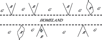
Figure 2: Schematic illustration of the result of a linear inoculation along a Petri dish of a small percentage (say, $2-5\%$) of mutant cells with both beneficial and deleterious mutants (labeled red, R and R’ respectively) with a majority of wild type (labeled green, G). (The width of the “homeland” between the two dashed lines is not relevant for this discussion, but is determined by the amount of fluid on the razor blade and the capillary length of the liquid culture). As discussed in the text, the opening angle $\Phi$ (shown for a beneficial mutation at the bottom) is given by the square root of the fitness advantage. The potentially obscuring effects of genetic drift in the linear boundaries of the beneficial mutant strains are not shown. Two deleterious mutants that have “surfed” successfully for a time at the population front are shown as well. These surfing events owe their very existence to genetic drift.

In this article, we develop a quantitative model of biological evolution at expanding frontiers, inspired by the microbiological experiments described above. Specifically, we focus on the sectoring dynamics after well-defined monochromatic domains have been established in the early stages of the experiment. Then, we argue that allele frequencies change due to the growth and shrinkage of sectors, which in turn reflects the competition of the deterministic force of natural selection and random number fluctuations (genetic drift).

Even in cases where the temporal variation of sector sizes is purely stochastic (no selection), a gradual decrease in the number of sectors is expected as the population expands. This coarsening process occurs because domains frequently lose contact to the wave front and no longer participate in the colonization process Fig. 5. In Sec. 3.1, we treat this form of neutral evolution using a simple model of annihilating random walkers, which allows us to predict the gradual decrease in the number of sectors as the colony grows. Both linear and radial inoculations are considered. Although our model predicts that one allele (genetic variant) dominates for linear inoculations, the number of surviving sectors remains finite at long times for radial expansions, in agreement with the experiments in Ref. (Hallatschek et al., 2007). In Sec. 3.2, we consider biased random walks to study the spread and ultimate fate of beneficial mutations arising at the front of a population, such as the one documented in Fig. 3. We relate the asymptotic sector angle to fitness differences and determine the rate at which beneficial mutations become established based on their mutation rate. Finally, we determine the genetic load due to deleterious mutations that accumulate in the course of a range expansion. Our analysis shows that, due to enhanced genetic drift, selection is quite ineffective in purging deleterious mutations from the invasion front. Finally, using a combination of theoretical arguments and computer simulations, we find that a critical mutation rate exists along a linear frontier beyond which the front population would inevitably decline in fitness. Depending on the details of the range expansion, our prediction for this error threshold can be much lower than the well-known result for well-mixed “zero-dimensional” populations.

The emergence of well-defined domain boundaries, which underlies our analysis, is not specific to range expansions in microbial systems, as we argue in Sec. 4, which contains conclusions and discussion. Instead, sharp boundaries appear naturally due to the reduction of dimensionality ($2$ to $1$) at the advancing front of a population spreading across a surface. Building on this hypothesis, we discuss to what extent our results generalize beyond microbial populations.

\psfrag{phi}{$\Phi$}\psfrag{x}{$x$}\psfrag{r}{$r_{0}$}\psfrag{R}{$r$}\psfrag{z}{$z$}\psfrag{M}{1mm}\includegraphics[scale={.5}]{benef-rc-1-1-13.8x-cropped.eps}

\psfrag{phi}{$\Phi$}\psfrag{x}{$x$}\psfrag{r}{$r_{0}$}\psfrag{R}{$r$}\psfrag{z}{$z$}\psfrag{M}{1mm}\includegraphics[scale={.5}]{rfp40cfpmut1_2_linear_cr_II-red-green-cropped.eps}

Figure 3: Beneficial mutations give rise to sectors with unusually large opening angles. a) This colony of yeast (S. cerevisiae) was grown from a 5:1 mixture of CFP (red) and RFP (green) labeled cells. The large funnel-like green sector, which arose spontaneously, outgrows both wild type strains. b) A linear inoculation of mixture of a CFP (red) strain that has a beneficial mutation compared to an otherwise neutral RFP (green) strain. The resulting sectors of CFP mutants have similar shape and are well separated due to the small ratio (1:40) of mutant to wild type.

\psfrag{y}{$P(x/\sigma)$}\psfrag{x}{$x/\sigma$}\includegraphics[scale={0.2}]{SF3.eps}

Figure 4: An illustration of the mechanism by which the sectoring pattern of a microbial colony coarsens in time. (a) Four monochromatic domains are bounded by a moving frontier (black line). (b) As the colony grows further in the upward vertical direction, the domain boundaries follow wandering paths. By chance, the two domain boundaries on the left-hand side meet. As a consequence, the enclosed domain (red left-hand domain in (b)) loses contact to the population front and is, henceforth, trapped in the bulk of the colony. We model these dynamics by replacing the tips of the domain boundaries by random walkers (blue circles) that “live” on the growing one dimensional edge of the colony. Even though these random walkers annihilate when they meet (yellow star), they have a non-zero survival probability on the growing circumference of a circular colony.

2 Materials and methods

Our null model for the sectoring dynamics rests on the assumption that the reproductive success of an individual is independent of its color. In other words, individuals with different alleles (genetic variants) have the same fitness. In a strictly neutral population mixture, domains should not grow on average, except for a linear increase in the radial direction due to the inflating frontier in the case of circular inoculations (Hallatschek et al., 2007). Even in the neutral case, however, sectors will exhibit variations in their sizes, because of inevitable chance effects during the reproduction process (genetic drift). The variations in sector sizes are manifest in the erratic path of the sector boundaries, see Figs. 1a,b. Apparently, these effects are much more pronounced for E. coli populations than for S. cerevisiae. Due to these fluctuations, neighboring domain boundaries can collide as the colony grows larger. As a result, the enclosed domain loses contact to the colonization frontier and is henceforth trapped in the bulk of the colony without further participation in the colonization process. Thus random fluctuations due to genetic drift are responsible for the continual reduction in sector number.

Our phenomenological model for these neutral dynamics is illustrated for a linear inoculation in Fig. 4. The meandering ends of domain boundaries are represented by random walkers that populate the expanding edge of the colony. The random walkers come in pairs, move along the advancing frontier and annihilate when they meet. Their trajectories in space and time describe the meandering and coalescing of domain boundaries visible in the microbial experiments of Fig. 1.

This model of annihilating random walkers with dynamics embodied in domain walls instead of the cells themselves serves as an effective description of the neutral evolutionary dynamics on long time and length scales (see discussion). The mathematical formulation of the model leads to generalized diffusion equations, which could be solved analytically.

The evolutionary dynamics changes dramatically when mutations arise close to the range margins of an expanding population that have non-negligible fitness effects. The funnel-like sector shape on the left side of Fig. 3, for example, is the result of a mutation that increased the rate of expansion in this particular green population compared to either its unmutated green relatives or the red population. A series of similar observations shows that beneficial mutation generically give rise to sectors with unusually large sector angles. This phenotype implies a bias in the diffusion process of the sector boundaries. To account effects of selection, we thus formulated a biased diffusion model for the domain boundary motion. This model was solved analytically in the limit of small mutation rates, and studied by means of spatially explicit simulations for larger occurrence rates of deleterious mutations.

3 Results

3.1 Neutral evolution

We first present scaling analysis for the emerging neutral coarsening dynamics, at both planar and curved fronts. The results of a more precise analytical calculation of the sectoring dynamics follows thereafter.

3.1.1 Scaling analysis

Consider the dynamics of the distance $X(r)$ between the tips of two neighboring domain walls within a linear frontier, such as in Fig. 1a. We assume that the domain boundary separation $X(r)$ is a continuous random variable  that fluctuates as if each domain boundary carried out an independent random walk with diffusion constant $D_{X}$. This assumption implies that if the average front position advances from $r_{0}$ to $r$ (see Fig. 1c) by a length increment $\Delta r\equiv r-r_{0}$, then the associated increment $\Delta X=X(r)-X(r_{0})$ in the domain size has zero mean and a variance $\sigma_{X}^{2}$ that grows linearly with distance $\Delta r$,

$$\left\langle\Delta X\right\rangle=0\;,\qquad\left\langle\Delta X^{2}\right\rangle=4D_{X}\Delta r\equiv\sigma_{X}^{2}\;.$$ (1)

Here, angular brackets denote an average over many realizations and the diffusion constant $D_{X}$ describes the wandering of a single wall and has units of length²/length. The extra factor of 2 arises in Eq. (1) because we look at the difference coordinate between two independent random walks . Note that Eq. (1) also implies a random walk in real time. Indeed, if the colony expands at a constant velocity $v$, we have $\Delta r=v\Delta t$ and may write Eq. (1) equivalently as

$$\sigma_{X}^{2}=4D_{X}v\Delta t=4\tilde{D}_{X}\Delta t\;.\quad\mbox{(constant expansion speed $v$)}$$ (2)

Thus, the random variable $X$ carries out a random walk in real time $t$ with diffusion constant $\tilde{D}_{X}\equiv D_{X}v$. In the following, we will employ $r$ as the effective time-like variable rather than the real time $t$. Although the expansion velocity $v$ will vary from organism to organism, and may even be time dependent during the early stages of a radial expansion (Murray, 2004), $v(t)$ drops out when the problem is formulated as in Eq. (1).

The random walk assumption, Eq. (1), forms the basic working hypothesis of our analysis of neutral evolution. As discussed in Ref. (Hallatschek et al., 2007), this assumption can be violated when the interface of the expanding population is rough, which can drive a super-diffusive wandering. This super-diffusion can also be analyzed on the scaling level, and we shall indicate the implied changes in Sec. 4. The diffusive scaling used here nevertheless captures the essential behavior of many models and has the advantage of being exactly solvable. Note that our neglect of the roughness of the interface allows us to characterize the position of the population front by a single time-like variable $r$ for both linear and circular inoculations (see Fig. 1).

A coalescence event occurs when two domain boundaries meet, and the enclosed domain is displaced from the wave front in favor of the neighboring domains. Equivalently, we can say that the tips of domain boundaries annihilate when they meet. The typical distance between domain walls that evade annihilation at distance $r$ should be comparable to the standard deviation $\sigma_{X}(r)$. Hence, we show that the average number $N(r|r_{0})$ of surviving lineages at effective time $r$ declines with increasing $\Delta r$ as the inverse of $\sigma_{X}$. Using a pre-factor derived below in the diffusion approximation, the number of sectors then is given by

$$N(r|r_{0})=\frac{L}{\sqrt{2\pi}\sigma_{X}}=\frac{L}{2\sqrt{2\pi D_{X}\Delta r}}\;,\quad\mbox{(linear inoculation)}$$ (3)

for a neutral $50:50$ mixture of two differently labeled but neutral sub-populations. In Eq. (3), $L$ is the total length of the population front. Note that microscopic length scales, such as the cell size (or, more generally, an initial domain size) do not appear in this asymptotic formula. The annihilation process eventually leads to the prevalence of only one domain, or allele, after the front advances a distance $\Delta r$ such that the distance between domain boundaries has become of order $L$. Although Eq. (3) is only approximate in this regime (see below), it correctly suggests $\Delta r\sim L^{2}/D_{X}$ as the order of magnitude of the fixation time for a linear inoculation.

In the case of an advancing curved population front, the ultimate fate of the gene pool is rather different. On top of the diffusion process, neighboring domain boundaries are subject to a deterministic expansion caused by the changing size of the perimeter of the population. Thus, diffusion competes with an antagonistic drift caused by the inflation of the perimeter, which inflates the distance between neighboring domain walls. Although the deterministic drift term will dominate on long times, diffusion dominates at earlier times.

Let us consider a circular colony as the simplest example of an advancing curved front. In this case, the perimeter grows linearly with the radius of the colony. This radial expansion tends to increase arc-length distances between domain boundaries. The ends of two neighboring domain boundaries drift apart at a speed proportional to their distance. Thus, two neighboring random walkers are subject to both deterministic drift and diffusion in the arc-length parametrization of their separation. Alternatively, we can describe the distance between two neighboring random walkers by their angular distance

$$\Delta\Phi\equiv\frac{\Delta X}{r}\;,$$ (4)

as indicated in Fig. 1d. This change of variables simplifies the problem to pure diffusion because sector angles remain unchanged on average during the growth of the colony. The angular diffusion constant $D_{\Phi}$ becomes, however, a decaying function of the radius $r$ of the colony,

$$D_{\Phi}(r)\equiv\lim_{\Delta r\to 0}\frac{\left\langle\Delta\Phi^{2}\right\rangle}{4\Delta r}=\lim_{\Delta r\to 0}\frac{\left\langle\Delta X^{2}\right\rangle/r^{2}}{4\Delta r}=\frac{D_{X}}{r^{2}}\;,$$ (5)

where $D_{X}$ is the diffusion constant that describes wall wandering for a linear inoculation, Eq. (1). When the colony grows from an initial radius $r_{0}$ to a final radius $r$, the mean square angular displacement changes by

$$\sigma_{\Phi}^{2}\equiv\left\langle\Delta\Phi^{2}\right\rangle=4\int_{r_{0}}^{r}\!\!dr^{\prime}\,D_{\Phi}(r^{\prime})=4D_{X}\left(r_{0}^{-1}-r^{-1}\right)\;.$$ (6)

Notice that the variance in angular distance depends on increments in inverse radii, as opposed to the linear dependence Eq. (1) for arc-length distances. An immediate consequence is that, when the colony grows much larger than the initial radius, $r/r_{0}\gg 1$, the expected mean square angular displacement stays finite, $\sigma_{\Phi}\to 2\sqrt{D_{X}/r_{0}}$. At long times, the sectoring pattern should therefore decompose into a finite number $N(\infty|r_{0})$ given by

$$N(\infty|r_{0})=\frac{L}{\sqrt{2\pi}\sigma_{\Phi}}=\sqrt{\frac{\pi r_{0}}{2D_{X}}}\;.\qquad\mbox{(circular inoculation)}$$ (7)

The numerical pre-factor in Eq. (7) again results from the quantitative analysis of the sectoring statistics in the diffusion approximation discussed below.

3.1.2 Sector size distribution for linear and radial expansions

According to our model, we can view successful sectors that do not get trapped behind the front as being bounded by random walks that evade any collision. The size distribution of sectors should therefore be determined by the positional distribution function of annihilating pairs of random walkers conditional on survival. Our goal is to determine this distribution quantitatively.

As in the scaling discussion, we measure time by the spatial position $r(t)$ of the frontier of the population. In the scaling discussion, we described the size of a sector by a distance $X(r)$ in the linear inoculation, and by an angle $\Phi(r)$ in the circular case. In order to capture both scenarios simultaneously, let us introduce a generalized sector size variable $Z(r)$, which is assumed to carry out a random walk with diffusion constant $D(r)$,

$$\left\langle\Delta Z\right\rangle=0\;,\qquad\left\langle\Delta Z^{2}\right\rangle=D(r)\Delta r\;.$$ (8)

The specific scenarios of linear and radial inoculations can be recovered by identifying

linear inoculation: $$Z=X\;,\qquad D(r)=D_{X}=\mbox{const.}$$ (9)

circular inoculation: $$Z=\Phi\;,\qquad D(r)=D_{\Phi}(r)=D_{X}/r^{2}\;.$$ (10)

The statistical properties of the sector size $Z(r)$ are described by a diffusion equation. Let $F(z,r|z_{0},r_{0})$ be the probability that $Z(r)=z$ when the front is at $r$ given that $Z(r_{0})=z_{0}$ at the earlier front position $r_{0}$. This distribution function satisfies

$$\partial_{r}F(z,r|z_{0},r_{0})=2D(r)\,\partial_{z}^{2}F(z,r|z_{0},r_{0})\;,$$ (11)

which is a direct consequence of Eq. (8) and the continuous nature of the random variable $Z(r)$ (van Kampen, 2001). To account for the possibility of annihilation, we impose an absorbing boundary condition at $z=0$,

$$F(0,r|z_{0},r_{0})=0\;.$$ (12)

The factor of two in front of the diffusion constant in Eq. (11) arises because $Z(r)$ is the distance between two random walkers. Also note that, in order to keep the analysis simple, we assume that space is unbounded in this section. Finite size effects can lead to the important effect of fixation as discussed in Sec. 3.1.3.

The absorbing boundary condition Eq. (12) can be fulfilled exactly by writing the solution as

$$F(z,r|z_{0},r_{0})=G(z,r|z_{0},r_{0})-G(-z,r|z_{0},r_{0})\;,$$ (13)

in terms of the solution $G(z,r|z_{0},r_{0})$ of the diffusion equation (11) without annihilation. Diffusion without annihilation, on the other hand, is well-known to be described by a Gaussian probability distribution,

$$g(\Delta z,\Delta r)\equiv G(z_{0}+\Delta z,r_{0}+\Delta r|z_{0},r_{0})=\frac{\exp\left(\frac{-\Delta z^{2}}{2\sigma^{2}}\right)}{\sqrt{2\pi\sigma^{2}}}\;,$$ (14)

where $\sigma$ is the standard deviation of the random variable $Z$ accumulated from frontier distance $r_{0}$ to distance $r$,

$$\sigma^{2}(r,r_{0})\equiv 4\int_{r_{0}}^{r}\!\!dr^{\prime}\,D(r^{\prime})=\left\{4D_{X}(r-r_{0})\mbox{ linear}\atop 4D_{X}(r_{0}^{-1}-r^{-1})\mbox{ radial}\;.\right.$$ (15)

This quantity was evaluated in the scaling analysis in Eqs. (1) and (6) for the linear and circular inoculation, respectively. Upon combining Eqs. (13) and (14), we obtain

$$F(z_{0}+\Delta z,r_{0}+\Delta r|z_{0},r_{0}) = g(\Delta z,\Delta r)-g(-2z_{0}-\Delta z,\Delta r)$$ (16)

$$= \frac{\exp\left(-\frac{\Delta z^{2}}{2\sigma^{2}}\right)}{\sqrt{2\pi\sigma^{2}}}\left[1-\exp\left(\frac{-2z_{0}(z_{0}+\Delta z)}{\sigma^{2}}\right)\right]\;.$$

This result can be used to predict the sector size distribution that emerges when a linear or circular colony grows from a finely divided mixture of differently labeled sub-populations. Suppose that the front of the colony advances from position $r_{0}$ to position $r>r_{0}$. Then, every point along the edge of the population sends out domain boundaries in a tree-like web that gradually coalesces, as illustrated in Fig. 5. Due to this coarsening process, the number of sectors $N(r|r_{0})$ at the front is a decreasing function of time $r$, whose ensemble average we seek to determine. Consider first an “infinite alleles model” (Hartl and Clark, 1997) where each cell of the founder population is labeled differently. In this case, each surviving sector at $r$ originates at earlier effective time $r_{0}$ in a single individual, the most recent common ancestor (denoted by a cross in Fig. 5).

\psfrag{t}{$r_{0}$}\psfrag{tau}{$r$}\includegraphics[scale={0.8}]{infinite-colors.eps}

Figure 5: A sketch of the sectoring pattern emerging from an (hypothetical) initial population in which each individual is labeled differently. The curved colony grows from initial radius $r_{0}$ to radius $r$. Each surviving lineage emerges from a single founder cell denoted by a cross.

Consequently, a sector is generated by two domain boundaries that start from the same location of the common ancestor at initial time $r_{0}$. Hence, the sector size distribution is simply given by the probability distribution function of random walkers that evade annihilation given that they start (almost) at the same place. This distribution can be obtained by normalizing the small $z_{0}$ expansion of $F(z,r|z_{0},r_{0})$ in Eq. (16). We thus obtain the sector size distribution

$$P(z,r|r_{0})=\frac{z}{\sigma^{2}}\exp\left(-\frac{z^{2}}{2\sigma^{2}}\right)\;,\qquad z\geq 0\;.$$ (17)

$P(z,r|r_{0})$ is the probability that a randomly chosen sector sampled at time $r$ has size $z$ in the infinite alleles model. The product $\sigma P$ is plotted as a function of the dimensionless variable $z/\sigma$ in Fig. 6 (dashed line). Note that Eq. (17) assumes that the population front is unbounded. For a circular inoculation, $0\leq z\leq 2\pi$, Eq. (17) is only valid in the limit $\sigma(r,r_{0})\ll 1$. The more complicated exact distribution for this bounded case, Eq. (39), is derived in Sec. 3.1.3 below.

The mean of the distribution Eq. (17) is given by

$$\left\langle Z(r|r_{0})\right\rangle = \sqrt{\frac{\pi}{2}}\sigma(r,r_{0})$$

$$= \left\{\sqrt{2\pi D_{X}(r-r_{0})}\qquad\mbox{(linear inoculation)}\atop\sqrt{2\pi D_{X}\left(r_{0}^{-1}-r^{-1}\right)}\qquad\mbox{(circular inoculation)}\;,\right.$$

and represents the average size of a sector. Equivalently, it is the average distance between two non-colliding random walkers that initially start out from (almost) the same place. The numerical pre-factor may be compared with the expected size $\sigma\sqrt{2/\pi}$ of a sector in the absence of annihilation, as can easily be shown from Eq. (14). Thus, the average separation of surviving annihilating random walks is a factor of $\pi/2\approx 1.57$ larger than of “phantom” random walks that can pass freely through each other. Intuitively, this factor represents an effective repulsion between two random walks that must avoid collision to survive.

The average number $N(r|r_{0})$ of sectors measured in many repeated experiments of a given kind (circular or linear), is given by the ratio of total size of the front $L$ and average sector size,

$$N(r|r_{0})=\frac{L}{\left\langle Z(r|r_{0})\right\rangle}=\sqrt{\frac{2}{\pi}}\frac{L}{\sigma}\qquad\mbox{(infinite alleles model)}\;.$$ (19)

Here, $L$ would be the total length of the population front for a linear inoculation. In the circular case, however, one would choose $L=2\pi$. The standard deviation then approaches $\sigma_{\Phi}=2\sqrt{D_{X}/r_{0}}$ for $r\to\infty$, so that $N(\infty|r_{0})=\sqrt{2\pi D_{X}/r_{0}}$. 

These results, however, only hold in the infinite alleles model. When we relax the assumption that every founder individual has a different color, the average number of sectors will be less. For instance, if the initial population is labeled by only two colors in equal proportions, as in the experiment in Ref. (Hallatschek et al., 2007), two neighboring sectors of the infinite alleles model will have the same color with probability $1/2$. Thus, there will be half as many sector boundaries as in the infinite alleles model. Accordingly, the average number of sectors in the two alleles model will be given by $N(r|r_{0})=L(r)/\left\langle 2Z(r|r_{0})\right\rangle$, which gives the pre-factors used in Eqs. (3) and (7) of our scaling analysis. More generally, we may consider an initially well-mixed population, in which two randomly chosen individuals have a different color with probability $H$, known as heterozygosity (Hartl and Clark, 1997). Then the number of sectors will be given by the result for the infinite alleles model, Eq. (19), multiplied by $H$.

\psfrag{y}{$\sigma P(z/\sigma)$}\psfrag{x}{$z/\sigma$}\psfrag{a}{$L/\sigma=1.5$}\psfrag{b}{$2.0$}\psfrag{c}{$2.5$}\psfrag{d}{$3.0$}\psfrag{e}{$3.5$}\psfrag{f}{$4.0$}\includegraphics[scale={0.8}]{glots-combined-normalized-to-1-fix-labeled.eps}

Figure 6: Sector size distribution predicted by the annihilating random walker model. The horizontal axis is the ratio of sector-size $z$ and the positional standard deviation $\sigma(r,r_{0})$ accumulated by a random walk between times $r_{0}$ and $r$, as defined in Eq. (15). Full lines represent exact solutions with the parameter $L/\sigma$ increasing in steps of $0.5$ in order of increasing peak height, as obtained from Eq. (39). For $L/\sigma\geq 4$, the exact solution is hardly distinguishable from the asymptotic result Eq. (17) (dashed line), which is independent of $L/\sigma$. The area under these curves represents the probability that a randomly chosen sector has not (yet) reached fixation. For small $L/\sigma\ll 1$, the area approaches $0$ because the fixation probability of a sector approaches $1$.

\psfrag{y}{$f(\sigma/L)$}\psfrag{x}{$\sigma/L$}\includegraphics[scale={0.8}]{fproba-vs-sigma.eps}

Figure 7: The graph describes how the probability of fixation depends on the amount of domain wall wandering. The function $f(\sigma/L)$ represents the probability that fixation is reached at a front of size $L$ given that the accumulated variance of a single domain boundary is $\sigma^{2}(r,r_{0})$, as defined in Eq. (15).

3.1.3 Finite front size - probability of fixation

Our previous results were derived under the assumption that the frontier is very large, or rather, that sectors are too small to “notice” that the front size is actually limited. However, when a sector grows up to a size comparable to the dimension $L$ of the front, we have to account for the possibility that the sector could take over the entire front and reach fixation. In this section, we determine the probability of fixation assuming periodic boundary conditions, as would be appropriate for a radial inoculation, or for microorganisms growing from a linear inoculation around the waist of a cylinder.

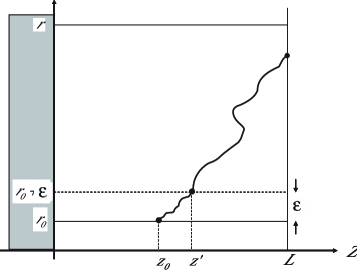
Figure 8: Graphical representation of Eq. (20) for the probability $u(r|z_{0},r_{0})$ a sector fixes at any frontier position up to and including $r$, given that the width $Z$ of the sector was $z_{0}$ at earlier frontier position $r_{0}$. Fixation occurs when the fluctuating width (black line) of a sector matches the system size $L$.

As a first step towards this goal, let us determine in the infinite alleles model the probability $u(r|z_{0},r_{0})$ that a sector has swept to fixation, $Z=L$, before the frontier has reached position $r$, given that the sector was a size $Z(r_{0})=z_{0}$ at initial “time” $r_{0}$. Here, $L=\pi d$, for a linear cylinder of diameter $d$, and $L=2\pi$ for a radial inoculation. To this end, it is convenient to derive from the diffusion equation Eq. (11) an equivalent differential equation for $u(r|z_{0},r_{0})$. This can be done, in analogy with derivations of the Kolmogorov backward equation in population genetics (Hartl and Clark, 1997), by writing

$$u(r|z_{0},r_{0})=\int\!\!dz^{\prime}\,u(r|z^{\prime},r_{0}+\epsilon)F(z^{\prime},r_{0}+\epsilon|z_{0},r_{0})\;,$$ (20)

which follows from the Markov property of the problem, see Fig. 8. Upon expanding the right hand side in $\epsilon$ and using Eq. (11), we obtain

$$u(r|z_{0},r_{0}) = \int{}{}{dz^{\prime}}\left[u(r|z^{\prime},r_{0})+\epsilon\partial_{r_{0}}u(r|z^{\prime},r_{0})\right]$$

$$\times\left[F(z^{\prime},r_{0}|z_{0},r_{0})+\epsilon 2D(r_{0})\partial_{z^{\prime}}^{2}F(z^{\prime},r_{0}|z_{0},r_{0})+\mbox{O}(\epsilon^{2})\right]$$

After noting that $F(z,r_{0}|z_{0},r_{0})=\delta(z-z_{0})$ and integrating by parts, we find

$$\partial_{r_{0}}u(r|z_{0},r_{0}) = -2D(r_{0})\partial_{z_{0}}^{2}u(r|z_{0},r_{0})$$ (22)

to order ${\cal O}(\epsilon)$. Note that all derivatives in Eq. (22) act on the coordinates $z_{0},r_{0}$ characterizing the initial conditions.

We seek a solution to Eq. (22) subject to the “final” condition $u(r|z_{0},r)=0$ (no fixation if the frontier does not advance), and two boundary conditions,

$$u(r|0,r_{0})=0\qquad u(r|L,r_{0})=1\;.$$ (23)

The first boundary condition accounts for the annihilation of a sector as $z_{0}\to 0$. The second guarantees that the fixation probability is 1 for all $r>r_{0}$ if the sector already spans the entire front at initial position $r=r_{0}$.

Note that the function $z_{0}/L$ satisfies both Eq. (22) and the boundary conditions Eq. (23), which motivates the following ansatz,

$$\Delta u(r|z_{0},r_{0})\equiv u(r|z_{0},r_{0})-z_{0}/L=\sum_{n=1}^{\infty}a_{n}(r_{0})W_{n}(z_{0})\;,$$ (24)

with coefficients

$$a_{n}(r_{0})=\int_{0}^{L}\!\!dz_{0}\,W_{n}(z_{0})\Delta u(r|z_{0},r_{0})\;,$$ (25)

given in terms of a complete orthonormal basis set of sine functions

$$W_{n}(z)=\sqrt{\frac{2}{L}}\sin(q_{n}z)\qquad q_{n}\equiv\frac{n\pi}{L}\;.$$ (26)

The function $\Delta u(r|z_{0},r_{0})$ represents the difference between the time-dependent solution, $u(r|z_{0},r_{0})$, and the linear steady state solution, $z_{0}/L$. The expansion of $\Delta u(r|z_{0},r_{0})$ in terms of sine-modes guarantees that the boundary conditions Eq. (23) are satisfied.

Inserting the ansatz Eq. (24) into Eq. (22) gives the evolution of the mode amplitudes $a_{n}(r_{0})$ with $r_{0}$,

$$\partial_{r_{0}}a_{n}(r_{0})=2q_{n}^{2}D(r_{0})a_{n}(r_{0})\;.$$ (27)

Upon integrating from $r$ to $r_{0}$, we obtain

$$a_{n}(r_{0})=a_{n}(r)e^{-q_{n}^{2}\sigma^{2}/2}\;,$$ (28)

with $\sigma=\sigma(r,r_{0})$ being the standard deviation defined in Eq. (15). The pre-factor $a_{n}(r)$ is determined by imposing the final condition $u(r|z_{0},r)=0$ on Eq. (25),

$$a_{n}(r) = \int_{0}^{L}\!\!dz_{0}\,W_{n}(z_{0})\;\Delta u(r|z_{0},r)$$ (29)

$$= -\sqrt{\frac{2}{L}}\int_{0}^{L}\!\!dz_{0}\,\sin(q_{n}z_{0})\frac{z_{0}}{L}$$ (30)

$$= \sqrt{\frac{2}{L}}\left\{{q_{n}^{-1}\;,\qquad n\mbox{ even}\atop-q_{n}^{-1}\;,\qquad\mbox{otherwise}}\right.\;.$$ (31)

Hence, the solution for the fixation probability of a sector of initial size $z_{0}$ reads

$$u(r|z_{0},r_{0})=\frac{z_{0}}{L}+\sum_{n=1}^{\infty}\frac{2(-1)^{n}}{q_{n}L}\sin\left(q_{n}z_{0}\right)e^{-q_{n}^{2}\sigma^{2}/2}\;.$$ (32)

Clearly, the absolute fixation probability goes to zero as the initial size $z_{0}$ of the sector decreases, because small sectors almost always get trapped by the absorbing boundary condition on the left side of Fig. 8.

In the infinite alleles model, we have an initially very large number $L/z_{0}$ of very tiny sectors, $z_{0}\to 0$, that all compete for taking over the colonization front. One and only one sector can reach fixation. In order to study the time dependent fixation probability of this successful sector we condition on ultimate survival. We ask, what is the probability that fixation is complete by the “time” $r$ provided that the conisdered sector reaches fixation? In the infinite alleles model, this probability follows from Eq. (32) after a normalization,

$$f(r|r_{0}) \equiv \lim_{z_{0}\to 0}\frac{u(r|z_{0},r_{0})}{u(\sigma\to\infty|z_{0},r_{0})}$$

$$= 1+2\sum_{n=1}^{\infty}(-1)^{n}e^{-q_{n}^{2}\sigma^{2}/2}$$

$$= \vartheta_{4}\left[0,\exp\left(\sigma^{2}\pi^{2}/(2L^{2})\right)\right]\;,$$ (34)

where $\vartheta_{n}[z,q]$ are the Jacobi theta functions. The function $f(r|r_{0})$ represents the probability that a colonization experiment running from time $r_{0}$ until time $r$ reaches fixation in the infinite alleles model. The denominator in Eq. (3.1.3) is a normalizing factor that ensures $f(r|r_{0})\to 1$ as $\sigma(r)\to\infty$. The dependence of $f(r|r_{0})$ on $\sigma/L$ is shown in Fig. 7.

At linear fronts, the accumulated standard deviation $\sigma=\sigma_{X}\propto\sqrt{\Delta r}$ increases without bound, so that fixation is inevitable at long times. For this case, (again restricting our attention to the infinite alleles model) we can determine the average “time” or frontier distance to fixation, $\left\langle\Delta r_{fix}\right\rangle$, by an integral over $f(r|r_{0})$,

$$\left\langle\Delta r_{fix}\right\rangle = \int_{r_{0}}^{\infty}\!\!dr\,(r-r_{0})\partial_{r}f(r|r_{0})$$ (35)

$$= \int_{r_{0}}^{\infty}\!\!dr\,\left[1-f(r|r_{0})\right]$$ (36)

$$= \frac{L^{2}}{12D_{X}}\;,\qquad\mbox{(linear inoculations)}$$ (37)

where we used Eq. (1) for the variance $\sigma_{X}^{2}$ and Eq. (34) to evaluate the integral in the second line, and the boundary condition $\lim_{r\to\infty}f(r|r_{0})\to 1$. Note that the pre-factor in Eq. (37) holds for periodic boundary conditions only, but can be evaluated for other boundary conditions along the same lines, see e.g. Ref.(Redner, 2007). Our derivation assumes the infinite alleles scenario, and we have not yet found an exact result for a finite number of colors. We expect, however, that the fixation time is linearly dependent on the heterozygosity $H$ of the initial population, at least for small heterozygosities. Our approximate argument is as follows. Suppose the initial population is an unbalanced binary mixture with $H\ll 1$. Then, with high probability $(1-H)$ the majority population will take over in a short time of order $(HL)^{2}/D$. On the other hand, with a low probability $H$ the colony will be taken over by the minority population, and this will take a time comparable to the fixation time $L^{2}/D$ in the infinite alleles model. As a consequence, these rare events of the fixation of the minority population dominate the avarage fixation time, which should therefore be of order $HL^{2}/D$.

Finally, we also generalize the sector size distribution Eq. (17) to finite-sized frontiers. To this end, we solve Eq. (11) under an additional absorbing boundary condition,

$$\left.F(z,r|z_{0},r_{0})\right|_{z=L}=0$$ (38)

which amounts to disregarding a sector once it reaches fixation. In Supplementary Text 1, we show that the solution to this problem can again be found in terms of the sine modes introduced in Eq. (26), specifically

$$F(z,r|z_{0},r_{0})=\frac{2}{L}\sum_{n=1}^{\infty}\sin(q_{n}x)\sin(q_{n}z_{0})e^{-q_{n}^{2}\sigma^{2}/2}\;.$$ (39)

As in the unbounded case, the sector size distribution is found by letting $z_{0}\to 0$,

$$P(z,r|r_{0})\propto\sum_{n=1}^{\infty}q_{n}L\sin(q_{n}x)e^{-q_{n}^{2}\sigma^{2}/2}\;.$$ (40)

In Fig. 6, we plot this sector size distribution normalized by the probability that a sector has not (yet) reached fixation. The results are indistinguishable from the asymptotic result Eq. (17) for $L/\sigma\leq 4$.

3.2 Natural selection

The above model can be extended to describe the effect of natural selection on mutations occurring during a range expansion, such as the one documented in Fig. 3. For simplicity, we remove complications associated with inflation by focusing on linear inoculations. In the previous section on neutral evolution, we ensured that each sector had the same chance of survival by requiring that the expected change in sector size vanishes, $\left\langle\Delta X\right\rangle=0$, see Eq. (1). This neutrality assumption is no longer valid if a sector is generated by mutants that have a different fitness than the wild type. To describe the fate of those non-neutral sectors, it is natural to assume that a selective advantage biases the sector growth. A sector harboring beneficial mutations will tend to increase its size, whereas a deleterious mutation will decrease the size. Upon setting $\Delta r=r-r_{0}$ as before, we thus generalize Eq. (1) to

$$\left\langle\Delta X\right\rangle=2m_{\perp}\Delta r\;,\qquad\left\langle\Delta X^{2}\right\rangle=4D_{X}\Delta r\;.$$ (41)

Here, we have assumed that selection does not alter the diffusion constant $D_{X}$, which seems reasonable, at least in the case of weak selection. The new parameter $2m_{\perp}$ describes the increase in the mean sector size due to selection and has units of a slope, length/length. The factor of $2$ indicates that each of the two boundaries exhibits an average lateral drift of $m_{\perp}$, adding up to a total sector growth rate of $2m_{\perp}$. In terms of measurable units, the bias parameter $m_{\perp}$ is given by the ratio of the velocity $v_{\perp}$ of a sector growth at right angles to the direction in which the front is advancing and the velocity $v$ of the wild type range expansion,

$$m_{\perp}\equiv\frac{v_{\perp}}{v}=\tan(\Phi/2)\;.$$ (42)

The second equality describes the relation between $m_{\perp}$ and the opening angle $\Phi$ of the sector at long times, which can be perceived from the sketch in Fig. 9. For weak selection, $\Phi$ will be small, and we can think of $m_{\perp}$ as being just half the (asymptotic) opening angle of the sector. This opening angle depends on the relation between the fitness effect of the mutation and the demographic expansion process.

Although the relation between $\Phi$ (or $m_{\perp}$) and selective advantage is complicated in general, it can be determined in two simple cases, both of which should be realizable for populations of microorganisms on a Petri dish, and for other range expansions as well. We assume that the only phenotypic effect of a beneficial mutation is an increase in the expansion velocity $\nu\to\nu^{\star}=f(s)\nu$, where $f(s)>1$. Here, $s$ is the usual selective advantage, defined as the ratio of growth rates $a^{\star}$ and $a$ of a population of organisms at the frontier, $a^{\star}/a=1+s$. In principle, $a$ (or $a^{\star}$) could be measured directly by monitoring cell divisions under a microscope, as was done in the sectoring experiments of Ref. (Hallatschek et al., 2007). However, the relation between the more easily measured front growth velocities and $s$ is known when population number fluctuations (i.e., effects of genetic drift) at the front are weak. One then expects the range expansions to be described by Fisher population waves (Murray, 2004), for which $v=2\sqrt{Da}$ and $v^{\star}=2\sqrt{D^{\star}a^{\star}}$, where $D$ and $D^{\star}$ are population diffusion constants at the frontier. If the beneficial mutation does not change the diffusion constant, we then have

$$f(s)=\sqrt{1+s}\;.$$ (43)

Wakita et al. have in fact measured a square root dependence of the growth velocity on the nutrient concentration in plates of bacillus subtilis (Wakita et al., 1994), consistent with Eq. (43) above when the growth rate is proportional to the nutrient concentration. Results are also known in the limit when genetic drift dominates growth at the frontier (Doering et al., 2003). In this limit, the growth velocities are proportional to doubling rates at the frontier. Assuming all other quantities are the same for the mutant and wild type, we then have

$$f(s)=1+s\;.$$ (44)

See Supplementary Text 2 for a more detailed discussion.

More generally, we expect that $f(s=0)=1$, and a Taylor series expansion about of the form

$$f(s)=1+cs+\dots$$ (45)

where $c>0$ and $s$ are small. Under the conditions described above, we have $c=1/2$ and $c=1$ for weak and strong genetic drift respectively.

Now suppose that a mutation arises (or a mutant cell is inserted by hand) close to the linear front of a wild type population in a Petri dish, and is able to overcome the critical initial phase, where selection is weak compared to genetic drift. For long times, the mutant sub-population will then form a sector that grows by the factor $f(s)$ faster into the unoccupied space than the wild type, as discussed above. Assume that, after initial transients, a time-independent sector angle forms. Again appealing to Fig. 9, we see that the mutant sector asymptotically approaches an opening angle $\Phi$ that satisfies

$$\cos(\Phi/2)=\frac{v}{v^{\star}}=\frac{1}{f(s)}\approx 1-cs\;.$$ (46)

Thus, for this “geometric” model of the opening angle $\Phi$, the drift parameter $m_{\perp}=v_{\perp}/v$ in Eq. (42) takes the form

$$m_{\perp}=\tan\left[\arccos\left(\frac{1}{f(s)}\right)\right]\approx\sqrt{2cs}\;,$$ (47)

where the approximations above assume $s\ll 1$.

It seems likely that this simple phenomenological model applies to the opening angles created by mutant strains of microorganisms on a Petri dish. Note that the square root dependence in Eq. (51) suggests that the sector angle could be a quite sensitive measure of weak selective differences. Other functional relations between and s are possible, however. As discussed in Appendix B, when number fluctuations are strong compared to the selective advantage at the front (strong noise limit), a linear relation arises in two-dimensional stepping stone models. These models allow some inter-diffusion of mutant and wild type strains after the population wave has passed by. A linear relation can also arise for the stochastic Fisher genetic waves generated associated with weakly deleterious mutations.

It remains to be seen experimentally which model most accurately describe the function $m_{\perp}(s)$ in a given situation. However, our parameterization of beneficial mutations in terms of the phenomenological parameter $m_{\perp}$ is quite generally applicable to any growth scheme leading to a bias $m_{\perp}$ in the random walk of domain boundaries. In the absence of a detailed microscopic understanding, one can always choose to parameterize beneficial and deleterious mutations directly in terms of $m_{\perp}$ itself. Although the arguments above focus on $m_{\perp}>0$, it is easy to see that deleterious mutations are described by $m_{\perp}<0$. In the following, we analyze the evolutionary consequences of this bias for both positive and negative values of $m_{\perp}$.

\psfrag{front}{frontier position}\psfrag{T}{time}\psfrag{M}{$v_{\perp}$}\psfrag{theta}{\hskip 5.69046pt$\Phi$}\psfrag{vstar}{$\propto v^{\star}\cos(\Phi/2)$}\psfrag{regular}{$\propto v$}\psfrag{tau}{$r$}\psfrag{t}{$r_{0}$}\includegraphics[scale={0.3}]{beneficial-sector-wiggly.eps}

Figure 9: A simple model of a beneficial sector within a planar wave front in the long-time limit. We assume that a beneficial mutation arises at front position $r_{0}$ and is able to overcome the short-time genetic drift at the front causing wobble in the domain boundaries. At long times the beneficial sub-population segregates and forms its own sector growing at radial velocity $v^{\star}$, which is assumed to be larger than wild-type growth speed $v$. Requiring that the kinks at the interface, where the wild type and mutant population meet, are reached by both populations at equal times, leads to $\cos(\Phi/2)=v/v^{\star}$.

3.2.1 Beneficial mutations, $m_{\perp}>0$

Isolated beneficial mutations are often lost due to genetic drift. However, because a sector of beneficial mutation tends to increase in size, $m_{\perp}>0$, its survival probability is increased compared to the neutral case. Here, we determine the fixation probability of a sector of beneficial mutations, and derive how frequently those sectors appear, given a certain rate of beneficial mutations.

Similar to the unbiased case, we will determine the fixation probability from a diffusion equation that describes the statistical properties of the size $X$ of a sector. Let $u(r|x_{0},r_{0})$ be the probability that a sector of beneficial mutations reaches fixation up to and including front position $r$ given that it had size $X(r_{0})=x_{0}$ at initial position $r_{0}$. Using analogous arguments to those in Sec. 3.1.3, it can be shown that the assumptions in Eq. (41) lead to a biased diffusion equation for the fixation probability $u(r|x_{0},r_{0})$, which reads

$$\partial_{r_{0}}u(r|x_{0},r_{0}) = -2D_{X}\partial_{x_{0}}^{2}u(r|x_{0},r_{0})-2m_{\perp}\partial_{x_{0}}u(r|x_{0},r_{0})\;.$$ (48)

Apart from the new drift term $\propto m_{\perp}$ this equation is identical to the unbiased case Eq. (22) with the constant diffusion parameter appropriate to linear inoculations. We again impose the boundary conditions of Eqs. (23) accounting for annihilation at $x=0$ and fixation at $x=L$, with the periodic boundary conditions appropriate to growth along a cylinder.

Because the diffusion constant and drift parameter are both independent of the time-like frontier position variable in the linear inoculation, we seek a $r_{0}$-independent solution of Eq. (22). After setting the right-hand side to zero and integrating twice, we find the steady state solution in the limit of long times, $r(t)\to\infty$,

$$u_{\parallel}(\infty|x_{0},r_{0})=\frac{1-e^{-m_{\perp}x_{0}/D_{X}}}{1-e^{-m_{\perp}L/D_{X}}}\;,$$ (49)

which is the ultimate survival probability of a beneficial mutation at a linear front .

The exponential dependence of Eq. (49) on $x_{0}$ implies that a sector almost certainly overcomes stochastic loss when it reaches a size larger than an “establishment length” $l\equiv D_{X}/m_{\perp}$. If a sector is much smaller than this characteristic length, $x_{0}\ll l$, the survival probability takes the simple form $u_{\parallel}\approx m_{\perp}x_{0}/D_{X}$ provided that $L/l\gg 1$. This result can be used to relate the frequency at which beneficial mutations become established in the form of sectors to the beneficial mutation rate $\tilde{\mu}_{b}$, which has units of an inverse time. To this end, we assume that all beneficial mutations confer the same selective advantage $m_{\perp}$, and consider the evolutionary dynamics during short effective “time” increments $\Delta r$, in which genetic drift is stronger than selection. According to the neutral results of Sec. 3.1, only a number $N(\Delta r)$ of front lineages evade stochastic loss during a time increment $\Delta r$. Equivalently we can say that there is at any time a set of $N(\Delta r)$ individuals whose descendants will be present after the next time increment $\Delta r$. Among this population of founders, beneficial mutations occur at rate $\mu_{b}N(\Delta r)$, where $\mu_{b}=\tilde{\mu}_{b}/v$ is the beneficial mutation rate in units of an inverse length. These mutations will ultimately survive at long times with probability $m_{\perp}x_{0}/D_{X}$, where $x_{0}=L/N(\Delta r)$ is the average size of a sector after time $\Delta r$. Multiplying these factors together yields the rate at which beneficial mutations become established

$$\mbox{Beneficial mutations establishment rate}=\mu_{b}Lm_{\perp}/D_{X}\;.$$ (50)

Note that the $\Delta r$-dependent sector number $N(\Delta r)$ drops out of the final result . Note also that the establishment rate is an inverse length in our choice of units, which has the following interpretation: It measures the number of beneficial mutations appearing per unit length of progression of the front. As discussed below, in situations where beneficial mutations are of the type proposed in Fig. 9, Eqs. (46) and (50) can form the basis of an experimental technique to measure the relative fitness advantage of beneficial mutations (as embodied in the parameter $m_{\perp}$) as well as beneficial mutation rates in microbial colonies.

3.2.2 Deleterious mutations, $m_{\perp}<0$

Given the importance of chance effects during population expansions, one may wonder to what extent deleterious mutations can prevail at expanding frontiers. Indeed, a recent simulation study (Travis et al., 2007) has observed deleterious mutations that are swept to high frequencies by population waves. It is easy to see how these “gene surfing” events of deleterious mutations may come about in one spatial dimension. The first step is a matter of chance. A deleterious mutation needs to arise close to the wave front and become frequent there, despite natural selection. Such surfing attempts are promoted by the strong genetic drift at expanding frontiers, which are characterized by small effective population sizes (Hallatschek and Nelson, 2008). Once the front has been taken over by a deleterious mutation, the population wave advances into empty territory at a somewhat reduced velocity $v^{\star}<v$ due to the reduced fitness of the mutants heading the expansion. The wild type population, on the other hand, is stuck in the bulk of the population, but nevertheless advances by displacing the less fit mutants. The ensuing genetic wave of advance may be described by a Fisher genetic wave (Fisher, 1937) with velocity $v_{g}$ (see Fig. 10). Although the wild type population tries to catch up with the front via this genetic wave, this will actually never happen if the genetic wave is slower than the population wave of the mutants, $v_{g}<v^{\star}$. Thus, deleterious mutations may take over permanently if $v^{\star}>v_{g}$. See Supplementary Text 2 for an example of a one dimensional model that exhibits this behavior over a broad parameter range.

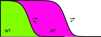
Figure 10: A deleterious mutation can permanently take over a population front in one spatial dimension if the speed of the genetic wave $v_{g}$ of the wild type (WT) invading the mutants (MT) is lower than the speed $v^{\star}$ of the advancing population front of mutants.

In two spatial dimensions, isolated deleterious mutations cannot permanently prevail at expanding frontiers. Although a sector harboring deleterious mutations may arise by chance effects as well, this sector is ultimately doomed to extinction because it has a lower expansion velocity than the surrounding wild type sectors. As a consequence, it is just a matter of time until the deleterious mutants are literally overtaken by the wild type population, see Fig. 2 and the time sequence illustrated in Fig. 11a. Nevertheless, deleterious mutations that temporarily surf on a population wave - until they finally “fall off” the wave front - pose a potentially serious threat to the pioneer population because they achieve much higher frequencies than expected under well-mixed conditions. As we demonstrate below, when these deleterious alleles become numerous, they can even trigger mutational meltdown in a cooperative manner.

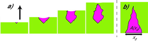
Figure 11: a) A deleterious mutation (red) arising close to the population front (black lines) achieves high frequency by temporarily “surfing” at the front. Figure b) defines the quantity $A(x_{0})$, which measures the expected area generated by a mutant sector if it has initial size $x_{0}$.

We seek to quantify the frequency of surfing deleterious mutations at expanding frontiers within the diffusion approximations used in this paper. As before, let $F(x,r|x_{0},r_{0})$ be the probability that a deleterious sector has size $X(r)=x$ at frontier position $r$, given that it had size $X(r_{0})=x_{0}$ at earlier “time” $r_{0}$. The biased diffusion equation for this distribution function $F(x,r|x_{0},r_{0})$ reads

$$\partial_{r_{0}}F(x,r|x_{0},r_{0})=-2D_{X}\partial_{x_{0}}^{2}F(x,r|x_{0},r_{0})+2\left|m_{\perp}\right|\partial_{x_{0}}F(x,r|x_{0},r_{0})\;.$$ (51)

This equation generalizes the unbiased Eq. (11), formulated backwards in time, and has the same form as Eq. (48) for the fixation probability $u(r|x_{0},r_{0})$ of a beneficial sector. The only difference is that the drift term has the opposite sign describing the shrinking of deleterious sectors.

We will now use equation Eq. (51) to study the statistical properties of the area $A(x_{0})$ spanned by a deleterious sector of initial size $x_{0}$ (see Fig. 11b). When combined with the mutation rate, this quantity turns out to control the steady state frequency of deleterious mutations at an advancing population front. On the “space-time” plot of two random walkers, where $r$ is the time-like coordinate in the growth direction, $A(x_{0})$ simply represents the area enclosed by the two colliding world lines, given they are initially separated by a distance $x_{0}$. The average area $\left\langle A(x_{0})\right\rangle$ can be expressed as an integral of $F(x,r|x_{0},r_{0})$ over its final coordinates,

$$\left\langle A(x_{0})\right\rangle=\int_{r_{0}}^{\infty}\!\!dr\,\int_{0}^{\infty}\!\!dx\,xF(x,r|x_{0},r_{0})\;.$$ (52)

To obtain a differential equation for $\left\langle A(x_{0})\right\rangle$, we multiply Eq. (51) by $x$ and integrate over $x$ and $r$,

$$\int_{r_{0}}^{\infty}\!\!dr\,\int_{0}^{\infty}\!\!dx\,x\,\partial_{r_{0}}F(x,r|x_{0},r_{0})=-2D_{X}\partial_{x_{0}}^{2}\left\langle A(x_{0})\right\rangle+2\left|m_{\perp}\right|\partial_{x_{0}}\left\langle A(x_{0})\right\rangle\;.$$ (53)

Because the left hand side represents the total derivative $\partial_{r_{0}}\left\langle A\right\rangle$ up to a boundary term evaluated at $r=r_{0}$, we have

$$\partial_{r_{0}}\left\langle A(x_{0})\right\rangle+\int_{0}^{\infty}\!\!dx\,xF(x,r_{0}|x_{0},r_{0})=-2D_{X}\partial_{x_{0}}^{2}\left\langle A(x_{0})\right\rangle+2\left|m_{\perp}\right|\partial_{x_{0}}\left\langle A(x_{0})\right\rangle\;.$$ (54)

Upon noting that $F(x,r_{0}|x_{0},r_{0})=\delta(x-x_{0})$ and that the expected mutant area $\left\langle A\right\rangle=\left\langle A(x_{0})\right\rangle$ is $r_{0}$-independent in linear inoculations, we obtain a simple ordinary differential equation for $\left\langle A(x_{0})\right\rangle$,

$$2D_{X}\partial_{x_{0}}^{2}\left\langle A(x_{0})\right\rangle-2\left|m_{\perp}\right|\partial_{x_{0}}\left\langle A(x_{0})\right\rangle+x_{0}=0\;.$$ (55)

This equation is solved by

$$\left\langle A(x_{0})\right\rangle=\frac{x_{0}^{2}}{4\left|m_{\perp}\right|}+\frac{D_{X}x_{0}}{2m_{\perp}^{2}}\;.$$ (56)

The quadratic contribution to the area, which dominates for $x_{0}\gg l=D_{X}/|m_{\perp}|$, is just the deterministic expectation for the area of the mutants neglecting genetic drift: With no diffusion of its boundaries, the deleterious sector should shrink laterally at a rate $2|m_{\perp}|$ and thus collapse when the front has advanced by $r_{c}=x_{0}/(2|m_{\perp}|)$. The deterministic sector area should thus equal the area $x_{0}^{2}/4|m_{\perp}|$ of an isosceles triangle with height $r_{c}$ and base $x_{0}$. Note that the characteristic length $l=D_{X}/|m_{\perp}|$ now plays the role of a “disestablishment length”.

The linear part in Eq. (56) is due to stochastic fluctuations and dominates on small scales, for $x_{0}\ll l$. As we now show, this stochastic part determines the mutational load of an expanding population. As in Sec. 3.2.1, we note that stochastic fluctuations dominate over selection on a small “time” scale $\Delta r$. There are at any time $N(\Delta r)$ founders - mutants or wild type - that give rise to sectors of average size $x_{0}=L/N(\Delta r)$ at a small time $\Delta r$ in the future. Among these $N(\Delta r)$ individuals deleterious mutations occur at a rate $N(\Delta r)\mu_{d}$, with $\mu_{d}=\tilde{\mu}_{d}/v$ representing the effective deleterious mutation rate per unit length of frontier growth. This process produces deleterious mutants at a rate given by

$$\mu_{d}N(\Delta r)\left\langle A[L/N(\Delta r)]\right\rangle\equiv\gamma L$$ (57)

For $\Delta r\to 0$, the short time neutrality assumption becomes exact, the factors of $N(\Delta r)$ cancel and we obtain

$$\gamma=\frac{D_{X}\mu_{d}}{2m_{\perp}^{2}}\;.$$ (58)

The restrictions of the footnote after Eq. (50) apply here as well, and we have assumed for simplicity that all deleterious mutations confer the same selective disadvantage $-|m_{\perp}|$.

The parameter $\gamma$ characterizes the mutational load. If $\gamma\ll 1$, it represents the fraction of the individuals in the newly colonized regions that carry the deleterious mutation. When the parameter $\gamma$ becomes of order one, mutant sectors become so numerous that they start to collide. These collisions are not captured by our simple theory, so $\gamma$ can no longer be interpreted literally as the fraction of mutants for $\gamma=O(1)$. Still, $\gamma$ defined by Eq. (58) can be viewed as a dimensionless control parameter that determines whether the pioneer population remains close to wild type or the mutational load becomes so strong that the average fitness deteriorates dramatically.

\psfrag{mperpmperp=0.1}{$m_{\perp}=0.1$}\psfrag{mperpmperp=0.01}{$m_{\perp}=0.01$}\psfrag{mperpmperp=0.04}{$m_{\perp}=0.04$}\psfrag{gamma}{$\gamma=\mu_{d}D_{X}/(2m_{\perp}^{2})$}\psfrag{pwt}{$p_{WT}$}\includegraphics[scale={0.5}]{x-summary-as-of-8-5-08-vs-gamma-paperfig.eps}

Figure 12: Simulation results for the fraction $p_{WT}$ of the wild type population for various values of the drift parameter $|m_{\perp}|$, characterizing the selective advantage of the wild type population, as a function of the dimensionless control parameter $\gamma=\mu_{d}D_{X}/(2m_{\perp}^{2})$. The simulations were carried out for small values of $m_{\perp}$ because our theoretical treatment applies to the limit of weak selection. To limit computational intensity, we restricted the simulations to $m_{\perp}>0.01$. Upper figure: With decreasing $m_{\perp}$, $p_{WT}(\gamma)$ seems to approach a universal function. The simulations confirm our analytical result that $1-p_{WT}\sim\gamma$ as $\gamma\to 0$, see inset. On the other hand, they also show that $p_{WT}\to 0$ above a critical threshold. The lowest probed value of $m_{\perp}=0.01$ indicates $\gamma_{c}=0.32\pm 0.02$. The simulation algorithm is described in Supplementary Text 3.

In fact, simulations for the simple model described in Supplementary Text 3 do indeed reveal a critical value $\gamma_{c}=0.32\pm 0.02$ that separates two regimes, see Fig. 12. For $\gamma<\gamma_{c}$, the average fraction of wild type surviving in a pioneer population stabilizes at a finite steady state value, whereas for $\gamma>\gamma_{c}$ the pioneer population keeps accumulating deleterious mutations until the wild type is lost entirely. This apparent continuous phase transition is the one dimensional spatial analog of the error threshold in well-mixed populations (M., 1971). Note that, depending on the functional relation between $m_{\perp}$ and the selective disadvantage $s<0$, the threshold value $\gamma_{c}$ for expanding populations can be very different from the well-known prediction $\gamma_{c}^{w.m.}=\tilde{\mu}_{d}/|s|=1$ for well-mixed populations. For the “geometric model” outlined at the beginning of Sec. 3.2, we have $m_{\perp}\propto\sqrt{s}$ and thus $\gamma_{c}\propto s^{-1}$ similar to a well-mixed population. However, for a two-dimensional stepping stone model in the strong noise limit, the relationship between $m_{\perp}$ and selective disadvantage $s$ is linear (cf. Supplementary Text 2). In this case, the genetic load $\gamma\propto s^{-2}$ could be strongly increased due to weakly deleterious alleles.

A simple argument suggests that the collision of mutant domains will indeed increase the expected fraction of mutants. Consider the collision of two mutant domains of sizes $x_{1}$ and $x_{2}$, characterized by the same selective disadvantage $|m_{\perp}|$. Then the newly combined domain has the increased size $x_{1}+x_{2}$. The expected area of the combined region as given by Eq. (56) is larger than the two separated domains by an amount

$$\left\langle A_{ex}(x_{1},x_{2})\right\rangle=\left\langle A(x_{1}+x_{2})\right\rangle-\left\langle A(x_{1})\right\rangle-\left\langle A(x_{2})\right\rangle=\frac{x_{1}x_{2}}{2|m_{\perp}|}\;.$$ (59)

This excess mutant area generated by the collision of domains furnishes a cooperative interaction associated with the mutational meltdown, as revealed in Fig. 12 as $\gamma\to\gamma_{c}$.

4 Conclusions and discussion

We have studied the impact of a continuous range expansion on the evolutionary dynamics of spatially structured populations. Our analysis focuses on the enhanced genetic drift at advancing frontiers, which leads to strong genetic differentiation. Most directly, our results apply to recent experiments on expanding microbial colonies (Hallatschek et al., 2007). However, we believe that the present analysis is of more general significance for populations that grow continuously and isotropically in two dimensions. The advancing frontier of those populations also has a thin layer of active pioneers, whose width depends on demographic parameters of the range expansion, such as the growth, migration and turnover rates. As the population advances, the pioneer population in this quasi-one dimensional front region is continuously re-sampled, as in a one-dimensional stepping stone model (Kimura and Weiss, 1964), for which it is known that allelic segregation occurs locally beyond a crossover time . Therefore, we believe that the coarsening process, and our model for it in terms of sharp domain boundaries, might be generally important for homogeneously expanding populations.

Within this model for population dynamics and genetic segregation of a continuous two-dimensional range expansion out of some prescribed initial habitat (linear or circular), we first studied the neutral genealogies of single loci without mutations. We found that only a fraction of founder cells are able to propagate their genes with the advancing front. Due to population turnover in the thin band of pioneers, the number of lineages gradually decreases as the expansion progresses. If a linear front advances by a distance $\Delta r$, the number of survivors decays like $1/\sqrt{\Delta r}$. One sector will dominate after an average fixation time $\propto L^{2}$, where $L$ is the linear dimension of the front. In the case of circular colonies, we find instead that a finite number of sectors survives, due to the geometric expansion of the perimeter which opposes genetic drift. For our moel, the expected number of these surviving sectors is proportional to the inverse square root of the initial radius of the colony. Both results assume that domain boundaries carry out a diffusive random walk. Growth models with surface roughness are expected to show an anomalously vigorous wall wandering (Saito and Muller-Krumbhaar, 1995; Hallatschek et al., 2007) where the variance in separation $X(r)$ between two walls grows as $(\Delta r)^{2\zeta}$ with an exponent $2\zeta>1$ as the front advances by a distance $\Delta r$. Our analysis of annihilating random walkers could be extended to these cases by assuming a diffusion “constant” that decreasing with the separation between the two random walkers . On the scaling level, such an analysis would yield an average sector number for linear inoculations increasing like $(\Delta r)^{-\zeta}$ instead of $(\Delta r)^{-1/2}$. For radial inoculation, the number of surviving sectors $N(\infty,r_{0})$ (see Eq. (7)) now scales with the initial radius according to $N(\infty,r_{0})\sim r_{0}^{1-\zeta}$. We speculate that the effect of inflation balancing genetic drift could be relevant for explaining the surprisingly large levels of genetic diversity among some invasive species, that have been introduced locally into a new and favorable habitats (e.g. rabbits in Australia). According to our model for radial expansions, those species are expected to preserve a considerable amount of their initial diversity during the habitat expansion.

Next, we considered the evolutionary dynamics of beneficial mutations arising at frontiers. To this end, we modified our model by adding a deterministic bias to the sectoring dynamics that tends to increase the size of sectors. This modification applies most directly to beneficial mutations whose only effect is to increase the growth rate of individuals $v\to v^{\star}=f(s)v$. We found that, at a linear frontier, a successful beneficial mutation “emits” a sector that has an opening angle $\Phi$ given by Eq. (46). If the change in velocity due to the mutations is weak, $s\ll 1$, then the sector angle is approximately given by $\Phi\approx 2\sqrt{2cs}$, where $c=1/2$ or $c=1$ depending on wether genetic drift is weak or strong at the front, respectively. The square root dependence on the selection coefficient indicates that sector angles are a sensitive measure of fitness differences. Thus, measuring sector-angles could be a useful tool to decipher the distribution of fitness effects of beneficial mutations, which can be difficult (or tedious) to measure by liquid culture techniques. The use of advancing population waves in evolutionary studies has been demonstrated earlier in a one-dimensional study of the effect of beneficial mutations on replicating RNA molecules (McCaskill and Bauer, 1993). In this study, beneficial mutations were identified by a spontaneous increase in expansion velocity of a Fisher population wave of proliferating RNA molecules travelling along a one-dimensional tube. In the two-dimensional extension of these studies, we expect a marked increase in resolution because we expect sector angles to be much more sensitive to selective changes than spreading velocities.

Although our parameterization of beneficial mutations in terms of the phenomenological parameter $m_{\perp}$ is quite generally applicable, the relation between bias $m_{\perp}$ and fitness difference remains to be assessed experimentally. The example of a beneficial mutation in Fig. 3 indeed seems to approach an asymptotic sector angle. The sector shape deviates initially somewhat from the simple triangular sector geometry used in our purely geometric model, however. This transient feature suggests that a number of other factors could change the relation between bias $m_{\perp}$ for small sectors and the fitness difference in microbial populations (Ron et al., 2003), such as a line tension penalizing front deformations. A related possibility is an effective attraction between oppositely directed Fisher genetic waves that slows down their separation at early times.

Finally, we estimated the mutational load in an expanding population. Deleterious mutations were found to proliferate at expanding frontiers rather differently than in well-mixed populations. Given that deleterious mutations with a selective disadvantage $|m_{\perp}|$ occur at a small rate $\tilde{\mu}_{d}$, we determined the fraction $\gamma$ of mutants at a linear wave front as $\gamma\equiv D_{X}\tilde{\mu}_{d}/(2vm_{\perp}^{2})$. Here, $v$ is the expansion velocity of the population wave, $D_{X}$ is the wall diffusion constant (in units of length${}^{2}/$length) and $m_{\perp}$ represents the “speed” or slope by which a single deleterious mutation is squeezed out of the population front. Furthermore, we presented numerical evidence that populations suffer from genetic meltdown as $\gamma\to\gamma_{c}\approx 0.32\pm 0.02$. This error threshold should be compared with the expectation $\gamma_{w.m.}=\tilde{\mu}_{d}/s$ for well-mixed populations (M., 1971), where $s$ is the relative fitness detriment of the deleterious mutations. Depending on the product $\gamma/\gamma_{w.m.}=D_{X}s/(2vm_{\perp}^{2})$, both predictions can be very different. If wall wandering represented by $D_{X}$ is strong, or the bias $m_{\perp}$ for a given fitness difference is weak (for instance $m_{\perp}\propto s$ as in the weak selection limit of the stepping stone model, cf. Supplementary Text 2, then the genetic load during a range expansion becomes substantially larger than in the well-mixed case. Thus, deleterious mutations could accumulate quite strongly during times of habitat expansions, thereby setting tight constraints on the dynamics of range expansions. Genetic load could be serious threat during general species invasions. This effect might extend to past range expansions of humans, as the mutational load inside Africa was found to be significantly lower than in the more recently colonized Europe (Lohmueller et al., 2008).

Acknowledgments: It is a pleasure to acknowledge helpful conversations with Nilay Karahan, Andrew Murray, Sharad Ramanathan, John Wakeley, and, in particular, Kirill Korolev, who suggested important corrections to the manuscript. The haploid strains (mating type a) of S. cerevisiae used for Fig. 3 were obtained through the generosity of John Koschwanez (FAS Center for Systems Biology, Harvard University), and are derived from a W303 strain and have either Cerulean (CFP) or mCherry (RFP) constitutively expressed from the ACT1 promoter and integrated at the ACT1 promoter locus. This research was supported by the German Research Foundation through grant no. Ha 5163/1 (O. H.), the National Science Foundation through Grant DMR-0654191, a National Institute of General Medical Sciences Grant, and the Harvard Materials Research Science and Engineering Center through Grant DMR-0213505 (D. R. N. and O. H.). Simulations were performed at the Center for Nanoscale Systems (CNS), a member of the National Nanotechnology Infrastructure Network (NNIN), which is supported by the National Science Foundation under NSF award no. ECS-0335765.

Appendix A Diffusion equation for periodic boundary conditions

In the main text, we gave a simple argument how to solve the diffusion equation (11) for annihilating random walks with absorbing boundary conditions at $z=0$. However, this solution is only strictly valid in unbounded space. Here, we derive the slightly more complicated solution Eq. (39) valid for finite systems. This solution satisfies another absorbing boundary condition, Eq. (38), which accounts for the fixation when the sector reaches the size of the system $L$.

We make the following ansatz

$$F(z,r|z_{0},r_{0}) = \sum_{n=1}^{\infty}a_{n}(r)W_{n}(z)$$ (A1)

$$a_{n}(r) = \int_{0}^{L}\!\!dz\,W_{n}(z)F(z,r|z_{0},r_{0})\;,$$ (A2)

where the sine mode $W_{n}(z)$ and wave numbers $q_{n}$ were defined in Eq. (26). This expansion in terms of sine-modes on the right-hand-side guarantees both boundary conditions.

Observe that the ansatz Eq. (A1) solves Eq. (11) provided that the mode amplitudes $a_{n}(r)$ obey

$$\partial_{t}a_{n}(r)=-2q_{n}^{2}D(r)a_{n}(r)\;.$$ (A3)

Integrating this from $r_{0}$ to $r$ gives

$$a_{n}(r)=a_{n}(r_{0})e^{-q_{n}^{2}\sigma^{2}/2}$$ (A4)

where $\sigma$ is the standard deviation in the $z$ coordinate, as defined in Eq. (15). The pre-factor is determined from the initial condition $F(z,r_{0}|z_{0},r_{0})=\delta(z-z_{0})$,

$$a_{n}(r) = \int_{0}^{L}\!\!dz\,W_{n}(z)F(z,r|z_{0},r_{0})$$ (A5)

$$= \sqrt{\frac{2}{L}}\sin(q_{n}z_{0})\;.$$ (A6)

Hence, the solution for the probability distribution reads

$$F(z,r|z_{0},r_{0})=\frac{2}{L}\sum_{n=1}^{\infty}\sin(q_{n}z)\sin(q_{n}z_{0})e^{-q_{n}^{2}\sigma^{2}/2}\;,$$ (A7)

which is Eq. (39).

Next, we would like normalize the distribution $F(z,r|z_{0},r_{0})$ by the total probability $\bar{u}(r|z_{0},r_{0})$ that a sector of initial size $z_{0}$ has not collapsed. This probability can be written as a sum of two terms,

$$\bar{u}(r|z_{0},r_{0}) = u(r|z_{0},r_{0})+\int_{0}^{L}\!\!dz\,F(z,r|z_{0},r_{0})$$ (A8)

$$= \frac{z_{0}}{L}+\frac{2}{L}\sum_{n=1}^{\infty}\frac{\sin(q_{n}z_{0})}{q_{n}}e^{-q_{n}^{2}\sigma^{2}/2}\;.$$ (A9)

The first term on the right hand side in Eq. (A8) is the probability that the sector has reached fixation, which was evaluated in Eq. (32), and the second term is the total probability that a sector has neither collapsed nor reached fixation. In the limit $z_{0}\to 0$, we can now construct the normalized distribution

$$P(z,r|r_{0})=\lim_{z_{0}\to 0}\frac{F(z,r|z_{0},r_{0})}{\bar{u}(r|z_{0},r_{0})}=\frac{\sum_{n=1}^{\infty}2q_{n}\sin(q_{n}z)e^{-q_{n}^{2}\sigma^{2}/2}}{\vartheta_{3}\left[0,\exp\left(\sigma^{2}\pi^{2}/(2L^{2})\right)\right]}\;.$$ (A10)

This limiting distribution is depicted in Fig. 6 for various values of $L/\sigma$. Note that the results are indistinguishable from the asymptotic result Eq. (17) for $L/\sigma\leq 4$. The area under these plots represent by construction the probability that a randomly chosen sector has not yet reached fixation.

Appendix B Genetic versus population waves

In this Appendix, we first exhibit an explicit model for the surfing of a deleterious gene in one dimension. Unlike the two-dimensional case considered in Ref. Travis et al. (2007), we focus here on one dimension, leading to the situation sketched Fig. 10. Provided we focus on populations that stop growing and diffusing once the population has passed by when $c+c^{\star}=1$ (see below), we can view this model as an approximation to the dynamics within the thin layer of actively growing pioneers in a two-dimensional range expansion, as in Fig.1a) and 1d). This approximation neglects number fluctuations at the front. The time variable $t$ in this Appendix then corresponds to the frontier position $r$ used elsewhere in this paper.

Let $c(x,t)$ be the dimensionless concentration of wild type individuals (growth rate $a$), and $c^{\star}(x,t)$ the dimensionless concentration of the mutant strain (growth rate $a^{\star}$). We assume for now $0<a^{\star}<a$, so that the mutation is deleterious relative to the wild type. We work in the strong selection limit, and neglect fluctuations in the number of discrete individuals within the two populations, although these can be important under some circumstances. For simplicity, we assume identical diffusion constants and a common steady state value or “carrying capacity” of unity in rescaled units for these two populations, both separately and when they are mixed together. The two populations differ in their growth rates, and in addition the wild type secrets a chemical that impedes the growth of the mutant under crowded conditions. A simple set of coupled reaction-diffusion equations for the two strains then reads,

$$\partial_{t}c = D\partial_{x}^{2}c+ac(1-c-c^{\star})-\alpha c^{\star}c\;,$$ (B1)

$$\partial_{t}c^{\star} = D\partial_{x}^{2}c^{\star}+a^{\star}c^{\star}(1-c^{\star}-c)+\alpha cc^{\star}\;.$$

“Crowded conditions” corresponds to $c+c^{\star}=1$, and the term $-\alpha c^{\star}c$ (with $\alpha>0$) in the first equation represents the secretion of an inhibitory chemical. Consider first the zero-dimensional case of well-mixed, spatially uniform populations, so that $c$ and $c^{\star}$ are a function of time only. It is straightforward to show that evolution of $c(t)$ and $c^{\star}(t)$ is then controlled by three fixed points, namely

$$(0,0)\mbox{, eigenvalues }a\;\&\;a^{\star}\mbox{ (unstable)}$$

$$(0,1)\mbox{, eigenvalues }-a\;\&\;\alpha\mbox{ (hyperbolic)}$$ (B2)

$$(1,0)\mbox{, eigenvalues}-a^{\star}\;\&\;-\alpha\mbox{ (stable)}$$

and that the invariant subspaces are $c=0,c^{\star}=0,c+c^{\star}=1$. The equal and opposite coupling strengths of the last terms in Eqs. (B1) were chosen to insure that $c+c^{\star}=1$ is an invariant subspace, and that we deal with the relatively simple situation that a composite population has the same carrying capacity as either population in isolation. The dynamics associated with this well-mixed effectively zero-dimensional population is shown in Fig. 13. If $a^{\star}\approx a>0$, both populations will grow up rapidly after a small inoculation near $(0,0)$. However, provided $0<\alpha\ll 1$ , the ultimate fate of the population is then a slow drift down the line $c+c^{\star}\approx 1$ until the wild type dominates at the stable fixed point $(1,0)$.

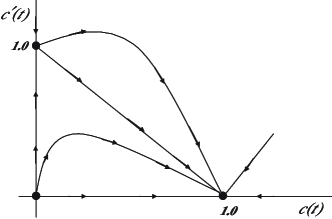
Figure 13: Dynamics associated with Eqs. (B) in zero dimensions, e.g., in a well-mixed overnight culture of microbes where spatial diffusion plays no role.

Now consider what happens in one spatial dimension. If the mutant strain is absent, ($c^{\star}(x,t)=0$), standard considerations Murray (2004) show that the remaining equation,

$$\partial_{t}c=D\partial_{x}^{2}c+ac(1-c)$$ (B3)

supports stable left- and right-moving waves that interpolate between $c(x,t)=0$ and $c(x,t)=1$ of the form

$$c(x,t)=f(x\pm vt)\;,$$ (B4)

with the velocity

$$v=2\sqrt{Da}$$ (B5)

and width $w=\sqrt{D/a}$. On the other hand, if $c(x,t)=0$ everywhere, the Fisher wave describing the mutant population $c^{\star}(x,t)$ has velocity

$$v^{\star}=2\sqrt{Da^{\star}}\;.$$ (B6)

Not surprisingly, the mutant Fisher population wave spreads with a lower velocity than the wild type, $v^{\star}<v$. However, consider now the situation when both strains are present and together always saturate the carrying capacity of the environment, i.e., we operate along the line $c(x,t)+c^{\star}(x,t)=1$. Equations Eq. (B1) then collapse to a single equation. If we focus on the dynamics of the wild type density $c(x,t)$, we now have

$$\partial_{t}c=D\partial_{x}^{2}c+\alpha c(1-c)\;.$$ (B7)

Equation Eq. (B7) describes a Fisher genetic wave of the wild type displacing a saturated population of mutants with a velocity

$$v_{g}=2\sqrt{D\alpha}\;,$$ (B8)

determined by $\alpha$, which represents the selective advantage under crowded conditions. Note that the Fisher genetic wave velocity is proportional to the square root of this selective advantage $\alpha$.

Figure 10 depicts in one dimension a superposition of a Fisher population wave on the right, with a mutant population moving into empty space with velocity $v^{\star}$, and a Fisher genetic wave on left, with the wild type displacing the mutant with velocity $v_{g}$. Successful “surfing” of a deleterious mutant ahead of the wild type requires only that the genetic wave not overtake the population wave, i.e., $v_{g}<v^{\star}$, which leads to the condition

$$\alpha<a^{\star}<a$$ (B9)

for this simplified model.

As discussed in the main text, the situation is considerably more complicated (and interesting!) in two dimensions, and when the genetic drift embodied in particle number fluctuations are taken into account. Let us focus now on a beneficial mutation forming a sector like that in Fig. 9. We consider the simple situation such that $a^{\star}\approx a$ (comparable Fisher population wave velocities), but assume that the wildtype is favored under crowded conditions, $\alpha<0$ with $|\alpha|\gg|a-a^{\star}|$. When the above deterministic two-component system reaction-diffusion model is generalized to two dimensions, it leads to a Fisher genetic wave velocity $v_{g}=2\sqrt{D|\alpha|}$, and a Fisher population wave velocities $v=2\sqrt{Da}\approx v^{\star}=2\sqrt{Da^{\star}}$. Assuming these waves are configured approximately at right angles as in Fig. 9, we obtain a $\sqrt{\alpha}$-dependence for the bias $m_{\perp}=v_{g}/v=\sqrt{\alpha/a}$ in the diffusion of the sector size, similar to Eq. (47). In analogy with Eq. (47) in the main text (with $c=1/2$), we set $\alpha\equiv\tilde{s}a$, thus defining a selective advantage $\tilde{s}$ under crowded conditions such that $a=a^{\star}$.

In contrast to Eq. (47), a linear dependence $m_{\perp}\propto\tilde{s}$ can result if the competition between the mutant and wild type is weak, $\tilde{s}\ll 1$. In this limit, selection is weak compared to genetic drift Doering et al. (2003), and the wave speed of a genetic Fisher wave is linear in $\tilde{s}$,

$$v_{g}=2\tilde{s}aD\tau_{g}c_{1d}/\Delta\;,\qquad\mbox{(weak selection)}$$ (B10)

where $D$ is the usual spatial diffusivity of the organisms, $c_{1d}$ is the effective one-dimensional population density at the frontier and $\tau_{g}$ is the generation time. The parameter $\Delta$ is the variance in offspring number in a single generation, and is in all breeding models a number of order one. Note that which relation between $m_{\perp}$ and the selection coefficients ($\tilde{s}$ or $s$) is realized strongly influences the genetic load, as predicted by Eq. (58).

Fisher population waves and Fisher genetic waves are approximately at right angles in the bacterial and yeast populations of Fig. 1. Here, $v\approx v^{\star}$ (so the population fronts advance into virgin territory at a common velocity) because these strains were chosen to be genetically neutral. There is no competition under crowded conditions, $\tilde{s}=0$, and the Fisher genetic waves in this Figure are stalled out on average. Note that the model Eq. (B1) and its generalization to two dimensions do not apply to regions far behind the population front of the microbiological experiments of Fig. 1., because the used micro-organisms not only stop growing, but also stop diffusing once the population wave has passed.

Appendix C Simulations of genetic load at expanding frontiers

In this section, we describe the simulations that were used to map out the genetic load at expanding frontiers as a function of the mutation rate, which is reported in Fig. 12. Our computer model is a derivative of the so-called contact process, which is believed to belong to the universality class of directed percolation Ódor (2004).

The simulation uses random sequential updates to evolve a one–dimensional lattice of binary variables ${\sigma_{i}}$, $i=1\dots N$, which can have the values WT (wild type) and MT (mutant). Initially, all sites are WT. At each time step, a pair of sites $\{\sigma_{i},\sigma_{i+1}\}$ is chosen such that periodic boundary conditions are respected. This pair of sites is then updated according to $\{\sigma_{i},\sigma_{i+1}\}\to\{\sigma^{\prime}_{i},\sigma^{\prime}_{i+1}\}$ with certain transition rates $w(\sigma^{\prime}_{i},\sigma^{\prime}_{i+1}|\sigma_{i},\sigma_{i+1})$. To describe the random occurrence of deleterious mutations, we implement

$$w(MT,.|WT,.)=w(.,MT|.,WT)=2D_{X}\tilde{\mu}_{d}\;,$$ (C1)

where the states not shown are arbitrary. To account for the biased random walk of domain boundaries,

$$w(WT,WT|WT,MT) = w(WT,WT|MT,WT)=(1+m_{\perp})/2$$ (C2)

$$w(MT,MT|WT,MT) = w(MT,MT|MT,WT)=(1-m_{\perp})/2\;.$$ (C3)

All other rates are zero. The expansion of domain boundaries is described by the first equation Eq. (C2), and the shrinkage by the second Eq. (C3). One lattice site in the simulation represents a length $2D_{X}$ of the linear frontier, and one time step corresponds to an equal change $\Delta r=2D_{X}$ in the frontier position, or effective time. The computer model then has the two non-dimensional parameters, $2D_{X}\tilde{\mu}_{d}$ and $m_{\perp}$.

We explore this model in the weak selection regime where the drift parameter $m_{\perp}\ll 1$ is small. This is the regime where the computer model generates domain boundaries that are well approximated by slightly biased continuous time random walks, as assumed in the main part of the paper. We find that the error threshold, at which the wild type is lost, only depends on the parameter $\gamma=D_{X}\tilde{\mu}_{d}/(2m_{\perp}^{2})$ introduced in Eq. (58) rather than on the two independent parameter of the computer model separately. This is documented by the data collapse in Fig. 12.

References

- Allee [1931] W. C. Allee. Co-operation among animals. Am. J. Soc., 37, 1931.
- Austerlitz et al. [1997] F. Austerlitz, B. JungMuller, B. Godelle, and P. H. Gouyon. Evolution of coalescence times, genetic diversity and structure during colonization. Theoretical Population Biology, 51:148–164, 1997.
- Barton et al. [2002] N. H. Barton, F. Depaulis, and A. M. Etheridge. Neutral evolution in spatially continuous populations. J. Theo. Popul. Biol., 61(1):31–48, FEB 2002.
- Biek et al. [2007] R. Biek, J. C. Henderson, L. A. Waller, C. E. Rupprecht, and L. A. Real. A high-resolution genetic signature of demographic and spatial expansion in epizootic rabies virus. Proc. Natl. Acad. Sci. U. S. A., 104(19):7993–7998, May 8 2007.
- Cavalli-Sforza et al. [1993] L. L. Cavalli-Sforza, P. Menozzi, and A. Piazza. Demic expansions and human-evolution. Science, 259:639–646, 1993.
- Crow and Kimura [1970] J. F. Crow and M. Kimura. An Introduction to Population Genetics Theory. 1970.
- Currat and Excoffier [2005] M. Currat and L. Excoffier. The effect of the neolithic expansion on european molecular diversity. Proceedings Of The Royal Society B-Biological Sciences, 272:679–688, 2005.
- Currat et al. [2006] M. Currat, L. Excoffier, W. Maddison, S. P. Otto, N. Ray, M. C. Whitlock, and S. Yeaman. Comment on ”Ongoing Adaptive Evolution of ASPM, a Brain Size Determinant in Homo sapiens” and ”Microcephalin, a Gene Regulating Brain Size, Continues to Evolve Adaptively in Humans”. Science, 313(5784):172a–, 2006.
- Doering et al. [2003] C. R. Doering, C. Mueller, and P. Smereka. Interacting particles, the stochastic Fisher–Kolmogorov–Petrovsky–Piscounov equation, and duality. Physica A: Statistical Mechanics and its Applications, 325(1-2):243–259, 2003.
- Edmonds et al. [2004] C. A. Edmonds, A. S. Lillie, and L. L. Cavalli-Sforza. Mutations arising in the wave front of an expanding population. Proc. Nat. Acad. Sci., 101:975–979, 2004.
- Elena and Lenski [2003] S. F. Elena and R. E. Lenski. Evolution experiments with microorganisms: The dynamics and genetic bases of adaptation. Nat. Rev. Gen., 4(6):457–469, 2003.
- Excoffier and Ray [2008] L. Excoffier and N. Ray. Surfing during population expansions promotes genetic revolutions and structuration. Trends in Ecology & Evolution, 23(7):347–351, 7 2008.
- Fisher [1937] R. A. Fisher. The wave of advance of advantageous genes. Ann. Eugenics, 7:355–369, 1937.
- Hallatschek and Korolev [2008] O. Hallatschek and K. Korolev. Genetic waves. 2008. in preparation.
- Hallatschek and Nelson [2008] O. Hallatschek and D. R. Nelson. Gene surfing in expanding populations. Theoretical Population Biology, 73(1):158–170, 2008.
- Hallatschek et al. [2007] O. Hallatschek, P. Hersen, S. Ramanathan, and D. R. Nelson. Genetic drift at expanding frontiers promotes gene segregation. Proceedings of the National Academy of Sciences, 104(50):19926–19930, 2007.
- Handley et al. [2007] L. J. L. Handley, A. Manica, J. Goudet, and F. Balloux. Going the distance: human population genetics in a clinal world. Trends in Genetics,, 23(9):432–439, 9 2007.
- Hartl and Clark [1997] D. L. Hartl and A. G. Clark. Principles of population genetics. Sinauer Associates Sunderland, Mass, 1997.
- Hewitt [2000] G. Hewitt. The genetic legacy of the quaternary ice ages. Nature, 405:907–913, 2000.
- Hewitt [1996] G. M. Hewitt. Some genetic consequences of ice ages, and their role in divergence and speciation. Biological Journal of the Linnean Society, 58(3):247–276, 1996.
- Keymer et al. [2006] J. E. Keymer, P. Galajda, C. Muldoon, S. Park, and R. H. Austin. Bacterial metapopulations in nanofabricated landscapes. Proceedings of the National Academy of Sciences of the United States of America, 103(46):17290–17295, Nov 14 2006.
- Kimura and Weiss [1964] M. Kimura and G. H. Weiss. Stepping stone model of population structure and decrease of genetic correlation with distance. Genetics, 49(4):561, 1964.
- Klopfstein et al. [2006] S. Klopfstein, M. Currat, and L. Excoffier. The fate of mutations surfing on the wave of a range expansion. Mol. Biol. Evol., 23:482–490, 2006.
- Le Corre and Kremer [1998] V. Le Corre and A. Kremer. Cumulative effects of founding events during colonisation on genetic diversity and differentiation in an island and stepping-stone model. Journal Of Evolutionary Biology, 11:495–512, 1998.
- Lohmueller et al. [2008] K. E. Lohmueller, A. R. Indap, S. Schmidt, A. R. Boyko, R. D. Hernandez, M. J. Hubisz, J. J. Sninsky, T. J. White, S. R. Sunyaev, R. Nielsen, A. G. Clark, and C. D. Bustamante. Proportionally more deleterious genetic variation in european than in african populations. Nature, 451(7181):994–997, 2008.
- M. [1971] Eigen M. Self-organization of matter and evolution of biological macromolecules. Naturwissenschaften, 58(10):465, 1971.
- McCaskill and Bauer [1993] JS McCaskill and GJ Bauer. Images of Evolution: Origin of Spontaneous RNA Replication Waves. Proc. Nat. Acad. Sci., 90(9):4191–4195, 1993.
- Murray [2004] J. D. Murray. Mathematical Biology I, chapter 11. Springer, 2004.
- Ódor [2004] G. Ódor. Universality classes in nonequilibrium lattice systems. Reviews of Modern Physics, 76(3):663–724, 2004.
- Phillips et al. [2006] BL Phillips, GP Brown, JK Webb, and R. Shine. Invasion and the evolution of speed in toads. Nature, 439(7078):803, 2006.
- Ramachandran et al. [2005] S. Ramachandran, O. Deshpande, C. C. Roseman, N. A. Rosenberg, M. W. Feldman, and L. L. Cavalli-Sforza. Support from the relationship of genetic and geographic distance in human populations for a serial founder effect originating in africa. Proc. Nat. Acad. Sci., 102:15942–15947, 2005.
- Redner [2007] S. Redner. A Guide to First-Passage Processes. Cambridge University Press, 2007.
- Ron et al. [2003] I. G. Ron, I. Golding, B. Lifsitz-Mercer, and E. Ben-Jacob. Bursts of sectors in expanding bacterial colonies as a possible model for tumor growth and metastases. Physica A: Statistical Mechanics and its Applications, 320:485–496, 2003.
- Rosenberg et al. [2003] N. A. Rosenberg, J. K. Pritchard, J. L. Weber, H. M. Cann, K. K. Kidd, L. A. Zhivotovsky, and M. W. Feldman. Response to comment on ”genetic structure of human populations”. Science, 300, 2003.
- Saito and Muller-Krumbhaar [1995] Y. Saito and H. Muller-Krumbhaar. Critical phenomena in morphology transitions of growth models with competition. Physical Review Letters, 74(21):4325–4328, May 22 1995.
- Templeton [2002] A. Templeton. Out of Africa again and again. Nature, 416:45–51, 2002.
- Travis et al. [2007] J. M. J. Travis, T. Munkemuller, O. J. Burton, A. Best, C. Dytham, and K. Johst. Deleterious mutations can surf to high densities on the wave front of an expanding population. Mol. Biol. Evol., 24(10):2334, 2007.
- van Kampen [2001] N. G. van Kampen. Stochastic processes in physics and chemistry. Elsevier Science, Amsterdam, 2001.
- Wakita et al. [1994] J Wakita, K. Komatsu, A. Nakahara, T. Matsuyama, and M. Matsushita. Experimental Investigation on the Validity of Population Dynamics Approach to Bacterial Colony Formation. J. Phys. Soc. of Japan, 63:1205, 1994.