Reducing the Bias and Uncertainty of Free Energy Estimates by Using Regression to Fit Thermodynamic Integration Data

Abstract

This report presents the application of polynomial regression for estimating free energy differences using thermodynamic integration. We employ linear regression to construct a polynomial that optimally fits the thermodynamic integration data, and thus reduces the bias and uncertainty of the resulting free energy estimate. Two test systems with analytical solutions were used to verify the accuracy and precision of the approach. Our results suggest that regression with a high degree of polynomials give the most accurate free energy difference estimates, but often with a slightly larger variance, compared to commonly used quadrature techniques. High degrees of polynomials possess the flexibility to closely fit the thermodynamic integration data but are often sensitive to small changes in data points. To further improve overall accuracy and reduce uncertainty, we also examine the use of Chebyshev nodes to guide the selection of non-equidistant $\lambda$ values for the thermodynamic integration scheme. We conclude that polynomial regression with non-equidistant $\lambda$ values delivers the most accurate and precise free energy estimates for thermodynamic integration data. Software and documentation is available at http://www.phys.uidaho.edu/ytreberg/software.

1 Introduction

Free energy constitutes an important thermodynamic quantity necessary for a complete understanding of most chemical and biochemical processes. Examples such as conformational equilibria and molecular association, partitioning between immiscible liquids, receptor-drug interaction, protein-protein, and protein-DNA association, and protein stability all require the underlying free energy profiles as the prerequisite for a complete comprehension of the intrinsic properties [4, 20, 21]. Indeed, the grand challenge of molecular modeling is to obtain the microscopic detail that is often inaccessible to conventional experimental techniques. Free energy is typically expressed as the Helmholtz free energy for an isothermal-isochoric system or the Gibbs free energy for an isothermal-isobaric system, respectively [4].

Thermodynamic integration (TI) has been widely employed to calculate free energy differences ($\Delta F$) between two well-defined systems [12, 18, 23, 24, 32]. It is a general scheme for the calculation of $\Delta F$ between two systems with potential energy functions $U_{1}$ and $U_{0}$, respectively. The free energy difference, $\Delta F=F_{1}-F_{0}$, is the reversible work done when the potential energy function $U_{0}$ is continuously and reversibly switched to $U_{1}$, and is defined as

$$\Delta F=-k_{B}T\ln\left(\frac{Z\left[U_{1}({\vec{R}})\right]}{Z\left[U_{0}({\vec{R}})\right]}\right),$$ (1)

where $k_{B}$ is the Boltzmann constant, $T$ absolute temperature of the system in Kelvin, and the configurational partition function is given by

$$Z\left[U({\vec{R}})\right]=\int e^{-U({\vec{R}})/k_{B}T}d{\vec{R}},$$ (2)

where ${\vec{R}}$ is the full set of configuration coordinates. TI is a method that computes the $\Delta F$ between two systems or states of interest by estimating the integral

$$\Delta F=\int_{\lambda=0}^{1}\left\langle\frac{\partial U_{\lambda}({\vec{R}})}{\partial\lambda}\right\rangle_{\lambda}d\lambda,$$ (3)

which is equivalent to the reversible work to switch from $U_{0}\to U_{1}$. The notation $\left\langle\cdot\right\rangle_{\lambda}$ represents an ensemble average at a particular value of $\lambda$. Switching the system between two potential energies requires a continuously variable energy function $U_{\lambda}$ such that $U_{\lambda=0}=U_{0}$ and $U_{\lambda=1}=U_{1}$. In addition, the free energy function $U_{\lambda}$ must be differentiable with respect to $\lambda$ for $0\leq\lambda\leq 1$ [14].

The relationship of eq. (3) is exact, but the integral must be approximated numerically by performing simulation at various discrete values of $\lambda$. Typically, these discrete $\lambda$ values are used to convert the integral to a sum (e.g., using quadrature). If the estimates of $\left\langle\cdot\right\rangle_{\lambda}$ include large fluctuations, then it is necessary to perform very long simulations in order to calculate the average value to sufficient statistical accuracy. In addition, the quantity $\left\langle\cdot\right\rangle_{\lambda}$ may heavily depend on $\lambda$ so that a large number of simulations at different $\lambda$ values is needed in order to estimate the integral with sufficient accuracy.

Typically researchers estimate $\Delta F$ with TI utilizing an arithmetic technique such as the trapezoidal or Simpson’s rule. These numerical methods work well if the curvature of the TI data is small. The trapezoidal rule, for example, approximates the area under the curve of a given function with a trapezoid. Thus, $\Delta F$ is approximated by summing the area of the trapezoids between $\lambda=0$ and 1. The trapezoidal rule is intrinsically simple to use and possesses the advantage that the sign of the error of the approximation can be determined. The trapezoidal rule will overestimate the integral of a function with a concave-up curve because the trapezoids include all the area under the curve as well as the extension above it. Similarly, an underestimate will likely to occur if the function reveals a concave-down curve because the areas is accounted for under the curve, but not above. However, the error is difficult to estimate if the curve includes an inflection point.

Importantly, the accuracy of $\Delta F$ using the trapezoidal rule can only improve by increasing the number of $\left\langle\cdot\right\rangle_{\lambda}$ even if the $\left\langle\cdot\right\rangle_{\lambda}$ have sufficiently converged. However, such a large number of long equilibrium simulations is not always feasible with limited computational resources.

We previously presented the successful application of polynomial and spline interpolation techniques for $\Delta F$ estimates via TI [26]. These techniques demonstrate superior accuracy and precision over trapezoidal quadrature, and give the best estimates of $\Delta F$ without demanding additional simulations. However, we also noted the inherent weakness and limitations of the interpolation techniques. The most important weakness is that high degree of interpolating polynomials suffer from Runge’s phenomenon, i.e., the approximation errors escalate rapidly as the degree of interpolating polynomial increases. This phenomenon is attributed to the fact that a data point at or near the middle of the interval gives a large contribution to the coefficients close to the endpoints. As a consequence, there is a tradeoff between having a better fit and obtaining a smooth well-behaved fitting polynomial [8, 10].

To alleviate these restrictions on polynomial order, we now introduce the polynomial regression technique for estimating $\Delta F$ using TI. Our goal is to reduce the bias and uncertainty in the estimates of $\Delta F$ from evaluation of the integral which is present even for infinite sampling (i.e., unbiased $\left\langle\cdot\right\rangle_{\lambda}$). Thus, we implemented the least squares method to construct the best-fit polynomial model, and used the Gaussian elimination method with partial pivoting and scaling to calculate the optimal coefficients for the polynomial. The best-fit polynomial model interpolates the free energy slope $\frac{dF}{d\lambda}=\left\langle\frac{\partial U_{\lambda}}{\partial\lambda}\right\rangle_{\lambda}$ as a function of $\lambda$. Unlike Lagrange and Newton interpolation techniques [26], regression permits the degree of polynomial to vary to better accommodate the curvature of $\frac{dF}{d\lambda}$ [8, 11, 31]. Two one-dimensional test systems with analytical solutions were constructed as the test cases to examine the accuracy and performance of the regression technique. We also investigated the use of Chebyshev nodes as non-equidistant $\lambda$ values for TI. The accuracy and precision of free energy estimates obtained from equidistant and non-equidistant $\lambda$ values are compared and contrasted. The results from our simulations suggest that regression, with sufficiently high degree of polynomials, can improve the accuracy and reduce bias for $\Delta F$ estimates without demanding additional simulation. Our study further shows that the use of non-equidistant $\lambda$ values further improves the accuracy and reduced uncertainty of the $\Delta F$ estimate over use of equidistant $\lambda$ values.

2 Theory

The primary objective of this study is to introduce the mathematical and statistical framework for the analysis of simulation data from TI using polynomial regression. The objective is to construct a regression model that best describes the simulation data, namely $\left\langle\frac{\partial U_{\lambda}}{\partial\lambda}\right\rangle_{\lambda}$, from each TI simulation at a fixed $\lambda$. The degree of the polynomial for the regression model is first determined, and best-fit coefficients are subsequently estimated using the least squares methods. In the context of free energy estimates using TI, the functional form of the simulation data is represented by a series of data points $\left\{\lambda,\frac{dF}{d\lambda}\right\}$, and the regression model is then constructed through these data points.

Regression attempts to delineate the relationship between independent (e.g., $\lambda$ values) and dependent variables (e.g., $\frac{dF}{d\lambda}$ estimates) by fitting a linear polynomial to the observed data points. The regression procedures construct a curve that optimally minimizes the errors between the estimated and observed values. It is important to note that, unlike Lagrange and Newton polynomial interpolations, regression does not mandate that $\lambda$ values cover the entire interval between 0 and 1. Instead, the $\lambda$ values can be chosen anywhere within $\left[0,1\right]$ because regression does not attempt to construct a curve that goes through every data point exactly. In other words, the polynomial model only describes the tendency and does not delineate the functional form of the data.

Mathematically, polynomial regression is used to fit data points to the equation $y=\beta_{0}+\beta_{1}x+\beta_{2}x^{2}+\ldots+\beta_{n}x^{n}$, where $\beta_{i}$ denotes the $i$th coefficient of the polynomial. The degree of polynomial, $n$, is independent of the number of data points. The higher order terms in polynomial equation have the greatest effect on the dependent variable (e.g., $\frac{dF}{d\lambda}$).

We used the least squares method, which is the most widely employed technique to calculate the best-fit coefficients for the construction of polynomial model [1]. It minimizes the sum of the squares of the deviations between the theoretical curve and the data points from simulations or empirical observations. A solution is thus obtained without the use of any iterative procedures. The solution to the construction of polynomial that best represents the data points is obtained by solving a system of linear equations generated from the minimization of errors between the true and approximated values. We utilize Gaussian elimination which is the most commonly used algorithm for solving systems of linear equations [9, 19]. Gaussian elimination with partial pivoting and scaling, in particular, offers superb numerical stability, and thus was used for the current study.

2.1 Mathematical Notation

Regression analysis generally refers to the study of the relationship between one or several predictors (independent variables we denote as $x$) and the response (dependent variable we denote as $y$). In the context of free energy estimates using TI, the simulation data is represented by a series of data points $\left\{\lambda,\frac{dF}{d\lambda}\right\}=\{x,y\}$, and the polynomial model is constructed through these data points. The following sections briefly describe the mathematical definitions and properties of the techniques, the least squares method and Gaussian elimination, for the construction of a polynomial model that best represents the free energy profile.

2.2 Least Squares Method

The least squares method is an approximation technique that constructs the best-fit curve for a set of data points based on the sum of squares of the errors. An error at a point is defined as the difference between the true and approximated values. Geometrically the best-fit curve is the one that minimizes the sum of squares of the vertical distances between the data points and the approximating curve (see Fig. 1 for an illustration). The least squares criterion has important statistical interpretations. If appropriate probabilistic assumptions about underlying error distributions are made, least squares produce the maximum likelihood estimate of the coefficients [1, 13]. The least squares method has an advantage over the Lagrange and Newton interpolation techniques [26] as the order of the approximation is independent of the number of data points. This allows the degree of polynomial to vary in order to accommodate the desired precision. Most importantly, least squares does not produce a polynomial that goes through each data point exactly. The curve that exactly fits all the data points incorporates all the error in the measurement into the model. Statistically, this is not a desirable outcome unless the data points have no error, which is unlikely [19].

Approximation using the least squares method can be achieved in either continuous or discrete forms. We used the discrete least squares method that is best with applications that have finite data. Specifically it is based on $m$ interpolated data points $\left[x_{i},y_{i}\right]$ for $i=0,1,2,\ldots,m$. The curve to be fitted is a polynomial $p\left(x\right)$ that best represents all data points (e.g., $\lambda$ values).

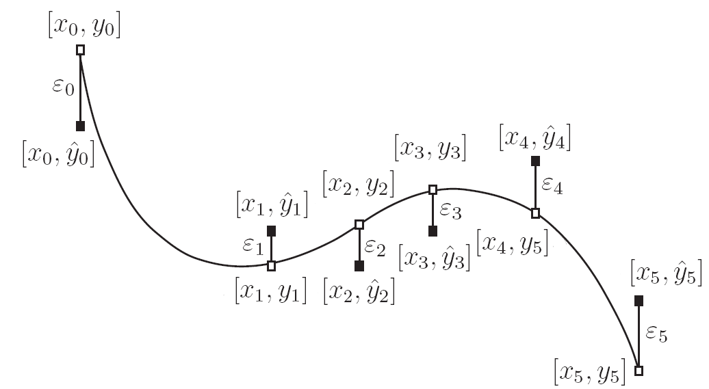
Figure 1: The least squares approximation technique. The least squares method constructs the best-fit curve that minimizes the sum of squares of the vertical distances (denoted by $\varepsilon_{0},\varepsilon_{1},\ldots,\varepsilon_{5}$) between the observed data points $\left[x_{0},\hat{y}_{0}\right],\left[x_{1},\hat{y}_{1}\right],\ldots,\left[x_{5},\hat{y}_{5}\right]$, and the estimates $\left[x_{0},y_{0}\right],\left[x_{1},y_{1}\right],\ldots,\left[x_{5},y_{5}\right]$ from the fitting line.

In the current study, the construction of a polynomial that best represents the $\lambda$ values was obtained by solving a system of linear equations generated from the minimization of errors between the true and approximated values. Mathematically the minimum of the sum of squares was found by setting the gradient to zero. The process was repeated and applied to all polynomial coefficients.

For example, consider a least squares approximation using a quadratic polynomial, $p\left(x\right)=\beta_{0}+\beta_{1}x+\beta_{2}x^{2}$, where $\beta_{i}$ refers to the $i$th coefficient of the polynomial for the regression model, produce a system of $3\times 3$ linear equations. The objective function, $\Psi$, that minimizes the sum of squares of the errors for the quadratic polynomial is expressed as

$$\Psi=\sum_{i=0}^{m}\left[y_{i}-\left(\beta_{0}+\beta_{1}x_{i}+\beta_{2}x_{i}^{2}\right)\right]^{2}.$$ (4)

The approximation is obtained by minimizing the sum of squares of the errors through $\frac{\partial\Psi}{\partial\beta_{0}}=0$, $\frac{\partial\Psi}{\partial\beta_{1}}=0$, and $\frac{\partial\Psi}{\partial\beta_{2}}=0$. The first equation is obtained through the steps,

$$\frac{\partial\Psi}{\partial\beta_{0}}=-2\sum_{i=0}^{m}\left[y_{i}-\left(\beta_{0}+\beta_{1}x_{i}+\beta_{2}x_{i}^{2}\right)\right]=0,$$

$$\sum_{i=0}^{m}y_{i}=\beta_{0}\sum_{i=0}^{m}1+\beta_{1}\sum_{i=0}^{m}x_{i}+\beta_{2}\sum_{i=0}^{m}x_{i}^{2}.$$ (5)

The second equation is generated in the same manner,

$$\frac{\partial\Psi}{\partial\beta_{1}}=-2\sum_{i=0}^{m}x_{i}\left[y_{i}-\left(\beta_{0}+\beta_{1}x_{i}+\beta_{2}x_{i}^{2}\right)\right]=0,$$

$$\sum_{i=0}^{m}x_{i}y_{i}=\beta_{0}\sum_{i=0}^{m}x_{i}+\beta_{1}\sum_{i=0}^{m}x_{i}^{2}+\beta_{2}\sum_{i=0}^{m}x_{i}^{3}.$$ (6)

Finally, the third equation is obtained from the steps

$$\frac{\partial\Psi}{\partial\beta_{2}}=-2\sum_{i=0}^{m}x_{i}^{2}\left[y_{i}-\left(\beta_{0}+\beta_{1}x_{i}+\beta_{2}x_{i}^{2}\right)\right]=0,$$

$$\sum_{i=0}^{m}x_{i}^{2}y_{i}=\beta_{0}\sum_{i=0}^{m}x_{i}^{2}+\beta_{1}\sum_{i=0}^{m}x_{i}^{3}+\beta_{2}\sum_{i=0}^{m}x_{i}^{4}.$$ (7)

The three equations can be formulated in the matrix form

$$\left[{\begin{array}[]{c c c}\sum\limits_{i=0}^{m}1&\sum\limits_{i=0}^{m}x_{i}&\sum\limits_{i=0}^{m}x_{i}^{2}\\ \sum\limits_{i=0}^{m}x_{i}&\sum\limits_{i=0}^{m}x_{i}^{2}&\sum\limits_{i=0}^{m}x_{i}^{3}\\ \sum\limits_{i=0}^{m}x_{i}^{2}&\sum\limits_{i=0}^{m}x_{i}^{3}&\sum\limits_{i=0}^{m}x_{i}^{4}\\ \end{array}}\right]\left[{\begin{array}[]{c}\beta_{0}\\ \beta_{1}\\ \beta_{2}\\ \end{array}}\right]=\left[{\begin{array}[]{c}\sum\limits_{i=0}^{m}y_{i}\\ \sum\limits_{i=0}^{m}y_{i}x_{i}\\ \sum\limits_{i=0}^{m}y_{i}x_{i}^{2}\\ \end{array}}\right].$$ (8)

These procedures can be generalized to a polynomial of arbitrary degree, $n$. In the context of free energy estimates using TI, the system of linear equations is written as

$$\left[{\begin{array}[]{c c c c c}\sum\limits_{i=0}^{m}1&\sum\limits_{i=0}^{m}\lambda_{i}&\ldots&\sum\limits_{i=0}^{m}\lambda_{i}^{n-1}&\sum\limits_{i=0}^{m}\lambda_{i}^{n}\\ \sum\limits_{i=0}^{m}\lambda_{i}&\sum\limits_{i=0}^{m}\lambda_{i}^{2}&\ldots&\sum\limits_{i=0}^{m}\lambda_{i}^{n}&\sum\limits_{i=0}^{m}\lambda_{i}^{n+1}\\ \ldots&\ldots&\ldots&\ldots&\ldots\\ \sum\limits_{i=0}^{m}\lambda_{i}^{n}&\sum\limits_{i=0}^{m}\lambda_{i}^{n+1}&\ldots&\sum\limits_{i=0}^{m}\lambda_{i}^{2n-2}&\sum\limits_{i=0}^{m}\lambda_{i}^{2n-1}\\ \sum\limits_{i=0}^{m}\lambda_{i}^{n+1}&\sum\limits_{i=0}^{m}\lambda_{i}^{n+2}&\ldots&\sum\limits_{i=0}^{m}\lambda_{i}^{2n-1}&\sum\limits_{i=0}^{m}\lambda_{i}^{2n}\\ \end{array}}\right]\left[{\begin{array}[]{c}\beta_{0}\\ \beta_{1}\\ \ldots\\ \beta_{n-1}\\ \beta_{n}\\ \end{array}}\right]=\left[{\begin{array}[]{c}\sum\limits_{i=0}^{m}\left\langle\frac{\partial U}{\partial\lambda}\right\rangle_{\lambda_{i}}\\ \sum\limits_{i=0}^{m}\left\langle\frac{\partial U}{\partial\lambda}\right\rangle_{\lambda_{i}}\lambda_{i}\\ \ldots\\ \sum\limits_{i=0}^{m}\left\langle\frac{\partial U}{\partial\lambda}\right\rangle_{\lambda_{i}}\lambda_{i}^{n-1}\\ \sum\limits_{i=0}^{m}\left\langle\frac{\partial U}{\partial\lambda}\right\rangle_{\lambda_{i}}\lambda_{i}^{n}\\ \end{array}}\right],$$ (9)

where $m$ refers to the number of TI simulations. Given the set of linear equations in eq. (9), we now need to solve these equations to obtain the polynomial coefficients that best fit the TI data. We chose to use Gaussian elimination with partial pivoting and scaling (see the next section for more details).

2.3 Gaussian Elimination

The solution to the system of linear equations has been an important numerical analysis problem as such a system arises in many different fields of research [30]. It is generally desirable to optimally fit a linear mathematical model to measurements obtained from simulations in order to obtain a better insight. The objective is then to extract predictions from the measurements and to reduce the effect of measurement errors. Numerical methods for solving linear systems are commonly classified as direct and iterative [19]. Linear least squares problems are solved by direct methods and admit a closed-form solution, in contrast to nonlinear least squares problems, which have to be solved by an iterative procedure. Direct methods yield the exact solution, assuming the absence of roundoff or other errors, in a finite number of elementary arithmetic operations. The fundamental method for direct solution is Gaussian elimination [30]. Gaussian elimination is an efficient and numerically stable algorithm that utilizes elementary row operations for the solution of systems of linear equations.

We used Gaussian elimination which is the most commonly employed algorithm to determine the solutions of a system of linear equations, to find the rank of a matrix, and to calculate the inverse of an invertible square matrix [1, 9, 19]. The Gauss-Jordan method, the matrix inverse method, the LU factorization method, and the Thomas algorithm are all modifications or extensions of the Gaussian elimination method [9, 29]. To achieve the optimal numerical stability, we incorporated the partial pivoting and scaling for solving the system of linear equations. Partial pivoting and scaling are particular important for free energy estimates using TI as numerical stability is of primary concern especially for a large number of simulations.

The elimination process involves normalizing the equation above the element to be eliminated by the element immediately above the element to be eliminated, which is called the pivot element, multiplying the normalized equation by the element to be eliminated, and subtracting the result from the equation containing the element to be eliminated. This process systematically eliminates terms below the major diagonal, column by column. This process is continued until all the coefficients below the major diagonal are eliminated. The elimination procedure fails immediately if the first pivot element is zero. The procedure may also fail if any subsequent pivot element is zero. Even though there may be non-zeros on the major diagonal in the original matrix, the elimination process may create zeros on the major diagonal. The simple elimination procedure therefore must be modified to avoid zeros on the major diagonal. This result can be accomplished by rearranging the equations, by interchanging equations (rows) or variables (columns), before each elimination step to put the element of largest magnitude on the diagonal. This process is referred to as pivoting. Interchanging both rows and columns is called full pivoting. Full pivoting is quite complex, and thus is rarely used [9, 19]. Interchanging only rows is called partial pivoting. Pivoting eliminates zeros in the pivot element locations during the elimination process. Pivoting also reduces roundoff errors, since the pivot element is a divisor during the elimination process, and division by large numbers introduces smaller roundoff errors than division by small numbers [9]. However, when the procedure is repeated, roundoff errors can still compound. This problem escalates rapidly as the number of equations increases.

The elimination process can indeed incur significant roundoff errors when the magnitudes of the pivot elements are smaller than the magnitudes of the other elements in the equations containing the pivot elements. In such cases, scaling is generally employed to select the pivot elements. The process of scaling involves normalizing all the elements in the first column by the largest element in the corresponding rows. Pivoting is then implemented based on the scaled elements in the first column, and elimination is applied to obtain zero elements in the first column below the pivot element. Similarly, before elimination is applied to the second column, all of the elements from 2 to $n$ are scaled, pivoting is implemented, and elimination is applied to obtain zero elements in column 2 below the pivot element. The procedure is applied to the remaining rows 3 to $n-1$. Back substitution is then applied to obtain the solutions. The effects of roundoff can be reduced by scaling the equations before pivoting. It is worth noting that scaling itself sometimes can introduce additional roundoff errors and should be used only to determine if pivoting is required. Scaling is generally not required if all the elements of the coefficient matrix are the same order of magnitude. For optimal numerical stability, we implemented the scaling algorithm to avoid pivoting to zero pivot elements [9, 28].

2.4 Chebyshev Nodes for Non-equidistant $\lambda$ Value Selection

Curve fitting with high degree of polynomials has not been a popular subject because such curves are particulary sensitive to small changes in the coefficients. Studies have shown that polynomial regression using equidistant abscissas, in particular, can give rise to convergence difficulties, especially with high degree of polynomials [8, 31]. A data point at or near the middle of the interval gives a large contribution to the values of $p\left(x\right)$ close to the endpoints. In other words, a small change to a data point in the middle can produce a significant excursion in the curve near the ends. The phenomenon is problematic with a set of a dozen or more data points that are more or less equidistant along the interval. Regression models with high order terms (typically higher than four) become more sensitive to the precision of coefficient values, where small differences in the coefficient values can result in a large differences in the computed $y$ value [8]. This difficulty intimates that high degree polynomials can be very sensitive to disturbances in the given values of the function.

Mathematically, equidistant curve fitting using polynomials of high degree is in some causes an ill-conditioned problem, especially in the outer parts of the interval $\left[x_{0},x_{m}\right]$ [5]. An ill-conditioned problem is one in which a small change in any of the elements of the problem causes a large fluctuation in the solution of the problem. For polynomial regression using the least squares method, for example, the coefficients in the matrix can vary over a wild range of several orders of magnitude. Since ill-conditioned systems are sensitive to small changes in the elements of the problem, they are also sensitive to roundoff errors. Werner [31] reported that special arrangements on the abscissae must be made in order to avoid the fluctuations on high degree of polynomials. Chebyshev nodes have been widely employed to counter the effects of such fluctuations [30]. Mathematically, Chebyshev nodes are derived from the roots of Chebyshev polynomial of the first kind, and tend to concentrate more heavily at the beginning and end of the interval. The use of Chebyshev nodes guarantees that the maximum error diminishes as the degree of polynomial increases [8].

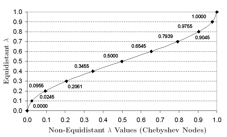
Figure 2: Transformation from equidistant to non-equidistant $\lambda$ values. The use of Chebyshev nodes for guiding the selection of non-equidistant $\lambda$ values aims to reduce the numerical instability of the regression as the degree of interpolating polynomial increases. For TI simulations, the non-equidistant $\lambda$ values are selected based on the expression $\lambda=\frac{1}{2}\left|\cos\left(\varphi\pi\right)-1\right|$.

For TI simulations, Chebyshev nodes (non-equidistant $\lambda$ values) are chosen using the following expression

$$\lambda=\frac{1}{2}\left|\cos\left(\varphi\pi\right)-1\right|,$$ (10)

for $\varphi\in\left[0,1\right]$. Chebyshev nodes possess the property that they become close together near the boundaries of the region (see Fig. 2 for an illustration). The use of Chebyshev nodes to guide the selection of non-equidistant $\lambda$ values aims to stabilize the polynomial construction processes. This is particularly important when the regression model includes a high degree of polynomial.

We note that several studies have reported the use of non-equidistant $\lambda$ values to improve the overall accuracy and precision of free energy estimate [2, 7, 16, 22, 25, 27]. However, it is important to realize that these studies used non-equidistant $\lambda$ values to better describe the curvature of the energy slope, while we are using non-equidistant $\lambda$ values to improve the numerical stability and accuracy of the construction of polynomials that fit the TI data.

2.5 Statistical Implications of Polynomial Modeling

Approximation of complex functions by polynomials is indeed a basic building block for a great many numerical techniques [30]. The degree of realism that needs to be incorporated into a model largely depends on the purpose of the regression analysis. The F-static is commonly employed to test the null hypothesis such as, $H_{0}:\beta_{q+1}=\beta_{q+2}=\ldots=\beta_{m-1}=0$, for $0\leq q\leq m$, for the adequacy of a model [19]. The least demanding purpose is the simple use of a regression model to summarize the observed relationship in a particular set of data points [1, 3]. There is no interest in the functional form of the model or in predictions to other sets of data or situations. The paramount concern is that the model adequately portrays the observed relationships. TI simulations data fall into this category.

It is very unlikely that the free energy changes diligently follows a particular functional form. However, it is crucial that the polynomial model closely fits the ensemble averages obtained from each TI simulation. The most demanding task using regression, on the other hand, is the esoteric development of mathematical models to accurately describe the physical, chemical, and biological processes in the system. The objective is to make the model as realistic as the state of knowledge will permit. Realistic models will tend to provide more protection against large errors from experiments or simulations. In the context of TI simulations, however, realistic models will likely mandate infinitely long simulations. Some authors [19, 5] reported that realistic models often may be simpler in terms of the number of coefficients to be estimated. A response with a plateau, for example, may require several terms of a polynomial to fit the plateau, but might be characterized very well with a two-coefficient exponential model.

3 Computational Details

Two test systems were constructed to analyze the accuracy and precision of the regression techniques for estimating $\Delta F$ using TI data. For the purpose of this study, it is important to use systems with an analytical solution in order to provide an objective analysis of the accuracy and precision of regression techniques. The first system involves two potential functions $U_{0}\left(\xi\right)=\frac{1}{2}\xi^{2}$ and $U_{1}\left(\xi\right)=2\left(\xi-5\right)^{2}$, where $\xi$ is the position of the particle, (see Fig. 3 for an illustration of the free energy curve) and the second system uses $U_{0}\left(\xi\right)=\frac{5}{2}\xi^{2}$ and $U_{1}\left(\xi\right)=\frac{1}{2}\left(\xi-5\right)^{2}$ (see Fig. 4 for an illustration of the free energy curve). The slope of $\frac{dF}{d\lambda}$ is considerably steeper for the second system and thus a much larger number of TI simulations would be required in order to achieve accuracy similar to that of the first system when using quadrature.

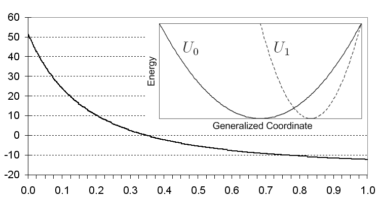
Figure 3: Free energy slope, $\frac{dF}{d\lambda}=\left\langle\frac{\partial U_{\lambda}}{\partial\lambda}\right\rangle_{\lambda}$, of the first one-dimensional test system obtained from TI simulations using 1001 equidistant $\lambda$ values. The figure on the top right corner shows that the potential energy functions, $U_{0}\left(\xi\right)=\frac{1}{2}\xi^{2}$ (solid line) and $U_{1}\left(\xi\right)=2\left(\xi-5\right)^{2}$ (dashed line), generate two offset harmonic wells with different curvature. The analytical solution of this system is $-\frac{1}{2}\ln\frac{1}{4}$.

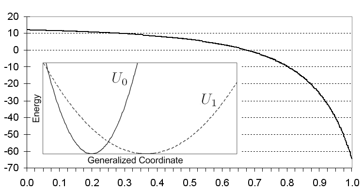
Figure 4: Free energy slope, $\frac{dF}{d\lambda}=\left\langle\frac{\partial U_{\lambda}}{\partial\lambda}\right\rangle_{\lambda}$, of the second one-dimensional test system obtained from TI simulations using 1001 equidistant $\lambda$ values. The figure on the bottom left corner shows that the potential energy functions, $U_{0}\left(\xi\right)=\frac{5}{2}\xi^{2}$ (solid line) and $U_{1}\left(\xi\right)=\frac{1}{2}\left(\xi-5\right)^{2}$ (dashed line), generate two offset harmonic wells with different curvature. The analytical solution of this system is $-\frac{1}{2}\ln 5$.

For our simulations, the switching function was defined as $U_{\lambda}\left(\xi\right)=\lambda U_{1}\left(\xi\right)+\left(1-\lambda\right)U_{0}\left(\xi\right)$. The non-equidistant $\lambda$ values are chosen according to the expression $\lambda=\frac{1}{2}\left|\cos\left(\varphi\pi\right)-1\right|$. The analytical solution of the $\Delta F$ for the first system is $-\frac{1}{2}\ln\frac{1}{4}$, and second $-\frac{1}{2}\ln 5$.

Simulations were performed with two sets of equidistant and non-equidistant $\lambda$ values, and TI simulations were performed at each value of $\lambda$. A total of 1,000 independent trials was run for each system. Simulations were performed for six and eleven equidistant and non-equidistant $\lambda$ values. An equal amount of simulation times (1,000,000 Monte Carlo steps) were used for each of six ($\lambda=0.0,0.2,0.4,0.6,0.8$, and $1.0$) and eleven ($\lambda=0.0,0.1,0.2,\ldots,0.9$, and $1.0$) equidistant values of $\lambda$. Identical TI simulations were performed on the corresponding non-equidistant $\lambda$ values, for six ($\lambda$ = 0.0, 0.0955, 0.3455, 0.6545, 0.9045, and 1.0) and eleven ($\lambda$ = 0.0, 0.0245, 0.0955, 0.2061, 0.3455, 0.5, 0.6545, 0.7939, 0.9045, 0.9755, and 1.0). Averages of the slope $\frac{dF}{d\lambda}=\left\langle\frac{\partial U_{\lambda}}{\partial\lambda}\right\rangle_{\lambda}$ were collected for each value of $\lambda$.

Each simulation started with an arbitrarily chosen initial position for the particle. Metropolis Monte Carlo [17] was performed using trial moves generated by adding a uniform random deviate between -0.5 and 0.5 to the current position. The acceptance ratio was maintained in the range of approximately 40 to 45% for each trial. Simulations were given 1,000 steps to equilibrate initially, then were allowed to proceed until the desired number of Monte Carlo steps (1,000,000) has been reached.

4 Results and Discussion

Table 1 summarizes averages and standard deviations of the biases for the estimates of $\Delta F$ from 1,000 independent trials on the first test system (see Fig. 3 for an illustration of the energy curve) using six equidistant and non-equidistant $\lambda$ values. We defined the bias as the difference between the analytical and estimated free energy. The bias from each independent trial was recorded, and averages and standard deviations were calculated for comparison. For higher degrees of polynomials, the estimates obtained from equidistant $\lambda$ values begin to diverge markedly. The averages and standard deviations of the biases fluctuate widely. This is largely due to the effects of overfitting. Overfitting occurs when a model contains too many parameters. An unrealistic model may fit perfectly if the model has enough complexity by comparison to the amount of data available. In other words, when the degrees of freedom in parameter selection exceed the information content of the data, this leads to arbitrariness in the final model parameter which reduces or destroys the ability of the model to generalize beyond the fitting data. The likelihood of overfitting depends not only on the number of parameters and data but also the conformability of the model structure with the data shape [1, 13, 6, 15]. This phenomenon, however, does not appear on the estimates obtained from simulations using the non-equidistant $\lambda$ values. Overall, the estimates of $\Delta F$ obtained from simulations using non-equidistant $\lambda$ values are considerably more accurate than that of equidistant $\lambda$ values. The estimates obtained from polynomials of degree six, for example, using non-equidistant $\lambda$ values are more accurate than that of degree ten using equidistant $\lambda$ values. It is worth noting that although the estimates obtained from polynomials of degree seven and higher show superior accuracy, these estimates, however, are no longer reliable as the number of parameters in the regression modes exceeds the number of $\lambda$ values.

Biases for $\Delta F$ estimates using six $\lambda$ values
for the first test system
	Equidistant $\lambda$		Non-equidistant $\lambda$
	Average	Std. Dev.	Average	Std. Dev.
Trapezoid	1.2490	0.0203	1.1398	0.0209
Degree 3	0.6893	0.0193	0.2520	0.0196
Degree 4	0.1599	0.0196	-0.0201	0.0211
Degree 5	0.1599	0.0196	-0.0201	0.0211
Degree 6	-0.6105	0.0426	-0.0296	0.0212
Degree 7	0.2537	0.0239	-0.0430	0.0213
Degree 8	2.3583	0.1555	-0.0150	0.0213
Degree 9	0.6152	0.0224	0.0032	0.0214
Degree 10	-3.4197	0.2292	-0.4076	0.0269

Table 1: Averages and standard deviation of the biases for the estimates of $\Delta F$ of the first test system (see Fig. 3 for an illustration of the energy curve) using six equidistant and non-equidistant $\lambda$ values. The degrees of polynomials vary from three to ten.

Biases for $\Delta F$ estimates using eleven $\lambda$ values
for the first test system
	Equidistant $\lambda$		Non-equidistant $\lambda$
	Average	Std. Dev.	Average	Std. Dev.
Trapezoid	0.3268	0.0145	0.3078	0.0154
Degree 3	0.3757	0.0144	0.2226	0.0146
Degree 4	0.0562	0.0143	0.0167	0.0152
Degree 5	0.0562	0.0143	0.0167	0.0152
Degree 6	0.0121	0.0150	0.0025	0.0154
Degree 7	0.0121	0.0150	0.0025	0.0154
Degree 8	0.0044	0.0166	0.0013	0.0155
Degree 9	0.0044	0.0166	0.0013	0.0155
Degree 10	0.0033	0.0347	0.0012	0.0155

Table 2: Averages and standard deviation of the biases for the estimates of $\Delta F$ of the first test system (see Fig. 3 for an illustration of the energy curve) using eleven equidistant and non-equidistant $\lambda$ values. The degrees of polynomials vary from three to ten.

Table 2 summarizes averages and standard deviations of the biases for the estimates of $\Delta F$ from 1,000 independent trials for the first test system (see Fig. 3 for an illustration of the energy curve) using eleven equidistant and non-equidistant $\lambda$ values. Overall, polynomial regression has made a significant improvement on the estimates using eleven $\lambda$ values. The results show that polynomials of degree eight seem sufficient to accurately estimate $\Delta F$. The estimates obtained from polynomials of higher degrees using equidistant $\lambda$ values, however, include much larger variation. As the degrees of polynomials increase, the standard deviations also increase. Using equidistant $\lambda$ values, higher degrees of polynomials are more likely to produce estimates with large fluctuations which inevitably degrade the overall accuracy and precision. This phenomenon reflects the fact that high degree of polynomials are sensitive to small changes in the data. Polynomial regression using non-equidistant $\lambda$ values, on the other hand, revels superior overall performance on the estimates of $\Delta F$. The estimates derived from polynomials using non-equidistant $\lambda$ values are much more accurate, and include much smaller variations. The standard deviations of the biases remain relatively constant. The overall estimates are much more accurate than that of equidistant $\lambda$ values. As an example, the estimates obtained from polynomials of degree six using non-equidistant $\lambda$ values are more accurate than that of degree ten using equidistant $\lambda$ values.

Table 3 summarizes averages and standard deviations of the biases for the estimates of $\Delta F$ from 1,000 independent trials using six equidistant and non-equidistant $\lambda$ values for the second test system (see Fig. 4 for an illustration of the energy curve). The estimates obtained from polynomials using equidistant $\lambda$ values are all heavily biased. For polynomials of higher degrees, the estimates become unreliable and include substantial variations. Similar to that of the first test system, overfitting causes the estimates of $\Delta F$ to fluctuate profoundly. For the estimates obtained from simulations using the non-equidistant $\lambda$ values, the estimates are still somewhat biased but greatly reduced from other estimates. As the degree of polynomials increases, the accuracy also improves accordingly. Since the second test system bears a much steeper energy curve, the variances of estimates are slightly larger than that of the first test system. It is clear that the use of non-equidistant $\lambda$ values gives much accurate estimates of $\Delta F$. This is apparently due to the fact that the use of non-equidistant $\lambda$ values significantly stabilize the polynomial construction processes and, subsequently, improve the overall accuracy.

Biases for $\Delta F$ estimates using six $\lambda$ values
for the second test system
	Equidistant $\lambda$		Non-equidistant $\lambda$
	Average	Std. Dev.	Average	Std. Dev.
Trapezoid	-1.8947	0.0236	-1.4949	0.0223
Degree 3	-1.2068	0.0221	-0.4202	0.0205
Degree 4	-0.3495	0.0212	0.0467	0.0218
Degree 5	-0.3495	0.0212	0.0467	0.0218
Degree 6	-0.7456	0.0623	0.0386	0.0218
degree 7	-0.2243	0.0363	0.0351	0.0218
Degree 8	0.2189	0.3169	0.0278	0.0219
Degree 9	-0.2006	0.0324	0.0260	0.0222
Degree 10	0.0571	0.5375	0.0306	0.0340

Table 3: Averages and standard deviation of the biases for the estimates of $\Delta F$ of the second test system (see Fig. 4 for an illustration of the energy curve) using six equidistant and non-equidistant $\lambda$ values. The degrees of polynomials vary from three to ten.

Biases for $\Delta F$ estimates using eleven $\lambda$ values
for the second test system
	Equidistant $\lambda$		Non-equidistant $\lambda$
	Average	Std. Dev.	Average	Std. Dev.
Trapezoid	-0.5076	0.0164	-0.4072	0.0158
Degree 3	-0.6552	0.0167	-0.3754	0.0150
Degree 4	-0.1257	0.0158	-0.0331	0.0154
Degree 5	-0.1257	0.0158	-0.0331	0.0154
Degree 6	-0.0325	0.0164	-0.0022	0.0157
Degree 7	-0.0325	0.0164	-0.0022	0.0157
Degree 8	-0.0116	0.0178	0.0012	0.0158
Degree 9	-0.0116	0.0178	0.0012	0.0158
Degree 10	-0.0051	0.0332	0.0016	0.0159

Table 4: Averages and standard deviation of the biases for the estimates of $\Delta F$ of the second test system (see Fig. 4 for an illustration of the energy curve) using eleven equidistant and non-equidistant $\lambda$ values. The degrees of polynomials vary from three to ten.

Table 4 summarizes the averages of biases for the estimates of $\Delta F$ obtained from 1,000 independent trials using eleven equidistant and non-equidistant $\lambda$ values for the second test system (see Fig. 4 for an illustration of the energy curve). With eleven rather than six $\lambda$ values, polynomials of degree eight seem sufficient to accurately estimate $\Delta F$ using either equidistant or non-equidistant $\lambda$ values. The estimates obtained from simulations using non-equidistant $\lambda$ values are generally more accurate than that of equidistant $\lambda$ values. It is worth noting that the estimates obtained from simulations using equidistant $\lambda$ values generally include much larger variations. This reflects that fact that high degrees of polynomials are more susceptible to oscillation. This is particular evident when the energy profile bears a steep curvature. Special arrangement for the $\lambda$ values should be made if one wishes to reduce the oscillation and improve the accuracy of approximation. Polynomial regression using non-equidistant $\lambda$ values shows superior overall performance. The estimates are considerably more accurate than that of equidistant $\lambda$ values. The use of non-equidistant $\lambda$ values reveals strong potential for the estimates of $\Delta F$ using polynomial regression. The estimates obtained from the trapezoidal quadrature using either the equidistant or non-equidistant $\lambda$ values, however, are still heavily biased.

5 Conclusion

We utilized polynomial regression to estimate free energy differences from thermodynamic integration simulation data. Two test systems were used to validate the accuracy and precision of the regression technique. The least squares method was used to extract vital information from each thermodynamic integration simulation and construct globally optimal polynomial model that best fits the free energy profile with respect to the switching variable $\lambda$. Gaussian elimination with partial pivoting and scaling was implemented to solve the resulting system of linear equations.

Results from the simulations clearly show that the use of regression with high degrees of polynomials gives the most accurate estimates of free energy differences. Although it is unlikely that the simulation data from thermodynamic integration will possess true polynomial representation, the flexibility of high degree polynomials allows the regression model to be approximated to any desired precision. Regression possesses the unique advantage that it permits the degree of polynomial to vary independently of the number of $\lambda$ values. This property significantly alleviate the restriction imposed by polynomial interpolation techniques such as Lagrange and Newton polynomial used in a previous study [26]. Estimates of $\Delta F$ for a large number of $\lambda$ values is there fore more straightforward. However, we caution that the degree of polynomial in regression model should be chosen to limit to a dozen or less to ensure numerical stability.

We also investigated the use of Chebyshev nodes (non-equidistant $\lambda$ values) for $\Delta F$ estimates and found that it improves the overall accuracy and reduces the biases compared to that of equidistant $\lambda$ values. Our results clearly demonstrate that the use of non-equidistant $\lambda$ values significantly reduces the variance, and improves the overall accuracy of the free energy estimates compared to that of equidistant $\lambda$ values. Our study has confirmed that the use of Chebyshev nodes to guide the choice of $\lambda$ values, in particular, offer superior numerical stability for regression analysis of TI data. Thus researchers are encouraged to use the polynomial regression and non-equidistant $\lambda$ values for their future free energy simulation using thermodynamic integration.

To allow researchers to immediately utilize the method, free software and documentation is provided via http://www.phys.uidaho.edu/ytreberg/software.

References

- [1] A. Björck. Numerical methods for least squares problems. SIAM, Philadelphia, PA, 1996.
- [2] A. Blondel. Ensemble variance in free energy calculations by thermodynamic integration: theory, optimal alchemical path, and practical solutions. Journal of Computational Chemistry, 25:985–993, 2004.
- [3] J.M. Chambers. Fitting nonlinear models: numerical techniques. Biometrika, 60:1–13, 1973.
- [4] C. Chipot and A. Phorille. Free energy calculations, theory and applications in chemistry and biology. Springer-Verlag, Berlin, Germany, 2007.
- [5] C.F. Crouse. On a point arising in polynomial regression fitting. Biometrika, 51:501–503, 1964.
- [6] H.T. Davis. Polynomial approximation by the method of least squares. The Annals of Mathematical Statistics, 4:155–195, 1933.
- [7] M. de Koning. Optimizing the driving function for nonequilibrium free-energy calculations in the linear regime: a variational approach. Journal of Chemical Physics, 122:104106, 2005.
- [8] J.D. Faires and R.L. Burden. Numerical methods. PWS-Kent Publishing Company, Boston, MA, 1993.
- [9] G.H. Golub and C.F. van Loan. Matrix computations. The Johns Hopkins University Press, Baltimore, MD, 3rd edition, 1996.
- [10] M.S. Henry. Approximation by polynomials: interpolation and optimal nodes. The American Mathematical Monthly, 91:497–499, 1981.
- [11] H. Jeffreys and B.S. Jeffreys. Lagrange’s interpolation formula. Methods of mathematical physics. Cambridge University Press, Cambridge, England, 3rd edition, 1988.
- [12] J.G. Kirkwood. Statistical mechanics of fluid mixtures. Journal of Chemical Physics, 3:300–313, 1935.
- [13] R. Kopitzke, T.J. Boardman, and F.A. Graybill. Least squares programs: a look at the square root procedures. The American Statistician, 29:64–66, 1975.
- [14] A.R. Leech. Molecular modeling, principle and applications. Pearson Education Limited, Harlow, Essex, UK, 2nd edition, 2001.
- [15] D.C. Lewis. Polynomial least square approximations. American Journal of Mathematics, 69:273–278, 1947.
- [16] A.E. Mark, W.F. van Gunsteren, and H.J.C. Berendsen. Calculation of relative free energy via indirect pathways. Journal of Chemical Physics, 94:3808–3816, 1990.
- [17] N. Metropolis, A.W. Rosenbluth, M.N. Rosenbluth, A.H. Teller, and E. Teller. Equation of state calculations by fast computer machines. Journal of Chemical Physics, 21:1087–1092, 1935.
- [18] T.Z. Mordasini and J.A. McCammon. Calculations of relative hydration free energies: a comparative study using thermodynamic integration and an extrapolation method based on a single reference state. Journal of Physical Chemistry, B, 104:360–367, 2000.
- [19] J.O. Rawlings, S.G. Pantula, and D.A. Dickey. Applied regression analysis. Springer-Verlag New York, Inc., New York, NY, 1998.
- [20] M.R. Reddy and M.D. Erion. Free energy calculations in rational drug design. Kluwer Academic/Plenum Publishers, New York, NY, 2001.
- [21] M. Sandal, F. Valle, I. Tessari, S. Mammi, E. Bergantino an F. Musiani, M. Brucale, L. Bubacco, and B. Samori. Conformational equilibria in monomeric -synuclein at the single-molecule level. PLoS Biology, 6:99–108, 2008.
- [22] T. Schmiedl and U. Seifert. Optimal finite-time processes in stochastic thermodynamics. Physical Review Letters, 98:108301, 2007.
- [23] M.R. Shirts and V.S. Pande. Comparison of efficiency and bias of free energies computed by exponential averaging, the bennett acceptance ration, and thermodynamic integration. Journal of Chemical Physics, 122:144107, 2005.
- [24] M.R. Shirts, J.W. Pitera, W.C. Swope, and V.S. Pande. Extremely precise free energy calculations of amino acid side chain analogs: comparesion of common molecular mechanics force fields for proteins. Journal of Chemical Physics, 119:5740, 2003.
- [25] S. Shobana, B. Roux, and O.S. Andersen. Free energy simulations: thermodynamic reversibility and variability. Journal of Physical Chemistry B, 104:5179–5190, 2000.
- [26] C. Shyu and F.M. Ytreberg. Use of polynomial interpolation to reduce bias and uncertainty of free energy estimates via thermodynamic integration. Journal of Chemical Theory and Computation, 0:ArXiv 0809.0882, 2008.
- [27] T. Steinbrecher. Nonlinear scaling schemes for lennard-jones interactions in free energy calculations. Journal of Chemical Physics, 127:214108, 2007.
- [28] G.W. Stewart. Introduction to matrix computations. Academic Press, New York, NY, 1973.
- [29] G.W. Stewart. Matrix algorithm: basic decompositions. SIAM, Philadelphia, PA, 1998.
- [30] E. Süli and D.F. Mayers. An introduction to numerical analysis. Cambridge University Press, Cambridge, UK, 2003.
- [31] W. Werner. Polynomial interpolation: Lagrange and Newton. Mathematics of Computation, 43:205–217, 1984.
- [32] F.M. Ytreberg, R.H. Swendsen, and D.M. Zuckerman. Comparison of free energy methods for molecular systems. Journal of Chemical Physics, 125:1–11, 2006.