Microlensing variability in the gravitationally lensed quasar
QSO 2237$+$0305 $\equiv$ the Einstein Cross

We present the continuation of our long-term spectroscopic monitoring of the gravitationally lensed quasar QSO 2237$+$0305. We investigate the chromatic variations observed in the UV/optical continuum of both quasar images A and B, and compare them with numerical simulations to infer the energy profile of the quasar accretion disk. Our procedure combines the microlensing ray-shooting technique with Bayesian analysis, and derives probability distributions for the source sizes as a function of wavelength. We find that the effective caustic crossing timescale is $4.0\pm 1.0$ months. Using a robust prior on the effective transverse velocity, we find that the source responsible for the UV/optical continuum has an energy profile well reproduced by a power-law $R\propto\lambda^{\zeta}$ with $\zeta=1.2\pm 0.3$, where $R$ is the source size responsible for the emission at wavelength $\lambda$. This is the first accurate, model-independent determination of the energy profile of a quasar accretion disk on such small scales.

1 Introduction

Soon after quasars were discovered, it was suggested that they are powered by the accretion of gas on to supermassive black holes at the centers of galaxies. Since the infalling matter has non-zero angular momentum, it forms a disk spinning around the central black hole (Lynden-Bell, 1969). Viscosity within the disk is thought to result in an outward transfer of angular momentum, thereby allowing the material to spiral gradually inward, heating the disk and causing it to emit intensely over a wide range of wavelengths (Shields, 1978).

Despite the numerous studies addressing the subject, there are still very few direct observational constraints on the spatial structure of quasar accretion disks. Quasars are located at cosmological distances, and it is particularly difficult to observe the inner regions of these objects. Direct imaging of the inner milli-parsec of a quasar would require angular resolutions on the order of micro- or even nano-arcseconds. There is currently no instrument capable of such performance. Fortunately, nature has provided us with a cosmic magnifying glass in the form of gravitational lensing, which helps to resolve the source, and to reveal the spatial structure of its most inner parts.

Our target is QSO 2237$+$0305. It was discovered by Huchra et al. (1985) during the Center for Astrophysics Redshift Survey, and is also known as “Huchra’s lens” or the “Einstein Cross”. It is probably the most studied gravitationally lensed quasar. It consists of a $z_{s}=1.695$ source gravitationally lensed into four images arranged in a cross-like pattern around the nucleus of a $z_{l}=0.039$ barred Sab galaxy. The average projected distance of the images from the lens center is $0.9$″.

Gravitational lensing is achromatic, in the sense that photons are deflected the same way regardless of their wavelength. However, lensing is sensitive to the source size, and quasar accretion disks are known to vary chromatically from the center to the edge. As a consequence, microlensing of the disk by stars located in the lensing galaxy will affect the quasar images independently, inducing chromatic differences in the spectra of the images (Wambsganss & Paczyński, 1991). These differences are directly linked to the energy profile of the disk, i.e. the scaling between the wavelength and the corresponding size of the source emitting at that wavelength. As a consequence, microlensing-induced flux variations can be used to constrain the energy profile of the quasar accretion disk.

Rauch & Blandford (1991) were the first to use this technique, and for the Einstein Cross, they found that the near-ultraviolet emission regions were smaller than expected for thermal emission from an accretion disk. However, more modern work in this system and other gravitational lenses have generally reached the opposite conclusion. For instance, Pooley et al. (2007) finds that the near-ultraviolet emission regions of ten lensed quasars are a factor of $3-30$ larger than the size predicted by simple accretion disk models to produce the observed optical flux. In a more quantitative analysis, Morgan et al. (2007) use the microlensing variability observed for nine gravitationally lensed quasars to show that the accretion disk size is consistent with the expectation from thin disk theory (Shakura & Sunyaev, 1973). However, these sizes are larger, by a factor of $\sim 3$, than the size needed to produce the observed infrared flux by thermal radiation from a thin disk.

The Einstein Cross is particularly well suited for microlensing studies, because of the symmetric configuration of the lensed images, which results in very short time delays, and because of the low redshift of the lensing galaxy, which places the lensed images in the bulge of the lensing galaxy, where the probability of microlensing by stars is high. Because of this, the Einstein Cross has been intensely monitored by different projects (e.g., Corrigan et al., 1991; Ostensen et al., 1996; Alcalde et al., 2002; Schmidt et al., 2002). The project having the longest duration and the best sampling rate is the Optical Gravitational Lensing Experiment (OGLE) (Woźniak et al., 2000a, b; Udalski et al., 2006). OGLE has monitored QSO 2237$+$0305 since 1997, and delivers the most complete lightcurves for this system.

Unfortunately, these monitoring campaigns are usually conducted in one photometric band, and hence they can be used to constrain the source size, but not the energy profile, which requires at least two bands. Multi-band monitoring is one approach, but even more effective is long-term spectrophotometric monitoring, as described in our first paper (Eigenbrod et al., 2008, paper I in the following). In this previous contribution, we describe our observations and data analysis, and report significant flux variations in the continuum and broad emission lines of the spectra of the four lensed images, indicating that both the continuum emitting region and the broad line region are microlensed.

Quasars are known to vary intrinsically, and in order to extract the microlensing-induced flux variations, we need to remove the intrinsic fluctuations from the lightcurves. In practice we do this by considering the difference between the light curves of two images. In the present study we focus on the lightcurves of images A and B, because they are the two images undergoing the strongest flux variations within the time span of our observations. In the case of QSO 2237$+$0305, we can neglect the time delays between the images, because they are expected to be on the order of one day or less (Schneider et al., 1988; Rix et al., 1992; Wambsganss & Paczyński, 1994). We also know that the observed flux $F$ of a lensed quasar image is the product of the unlensed flux $F_{0}$ of the source, the extinction $e^{-\tau}$, and the macro and micro-magnification $\mu_{macro}$ and $\mu_{micro}$

$$F=\mu_{micro}\leavevmode\nobreak\ \mu_{macro}\leavevmode\nobreak\ e^{-\tau}\leavevmode\nobreak\ F_{0}\leavevmode\nobreak\ \textrm{.}$$

As observed in paper I, image A is affected by long-term (more than 5 years) microlensing. Hence the micro-magnification $\mu_{micro}$ has two components over the time span of our observation: one constant long-term magnification $\tilde{\mu}_{micro}$, and one variable short-term $\mu^{\prime}_{micro}(t)$

$$\mu_{micro}(t)=\mu^{\prime}_{micro}(t)\leavevmode\nobreak\ \tilde{\mu}_{micro}\leavevmode\nobreak\ \textrm{.}$$

We shall mention that this separation in long and short-term microlensing is purely empirical, and only reflects the impossibility of retrieving the intrinsic source flux. The difference in magnitude $\Delta m$ between image A and B is given by $\Delta m=-2.5\log(F_{A}/F_{B})$. As observed in paper I, the extinction remains constant in time in all four images of the Einstein Cross. The macro-magnification given in Table 3 results in a constant magnitude difference on the order of $-0.1$ mag between images A and B. As a consequence, the time variability that we observe in $\Delta m$ is only due to short-term microlensing

$$\Delta m=-2.5\log\left(\frac{\mu^{\prime}_{micro,A}}{\mu^{\prime}_{micro.B}}\right)+m_{0}$$

where $m_{0}$ is a constant. Microlensing depends on the source size. Smaller sources are more strongly affected by microlensing than larger sources. We also know that bluer photons are emitted closer to the center of a quasar than redder ones. Hence we expect stronger variations of $\Delta m$ at bluer wavelengths (Wambsganss & Paczyński, 1991).

In this paper, we use this chromatic behavior of microlensing to compare the observed variability of $\Delta m$ at different wavelengths with numerical simulations. Using Bayesian analysis similar to Kochanek (2004) and Anguita et al. (2008), we derive the probability distributions for the size of the source emitting at a given wavelength. This eventually defines the energy profile of the quasar accretion disk.

In the following, we consider a flat cosmology with $(\Omega_{m},\,\Omega_{\Lambda})=(0.3,\,0.7)$ and $H_{0}=70$ km s^-1 Mpc^-1.

Table 1: Journal of the second part of our spectroscopic monitoring of QSO 2237$+$0305. The Julian dates are given in HJD-2450000.

ID	Civil Date	HJD	Mask	Seeing $[\arcsec]$	Airmass
32	10$-$07$-$2007	4292	1	0.63	1.153
			2	0.55	1.132
33	15$-$07$-$2007	4297	1	0.57	1.158
			2	0.54	1.220
34	25$-$07$-$2007	4307	1	0.79	1.231
			2	0.83	1.161
35	03$-$08$-$2007	4316	1	0.68	1.412
			2	0.68	1.278
36	27$-$08$-$2007	4340	1	0.88	1.133
			2	0.89	1.143
37	06$-$09$-$2007	4350	1	0.67	1.396
			2	0.72	1.252
38	20$-$09$-$2007	4364	1	0.73	1.230
			2	0.83	1.167
39	23$-$09$-$2007	4367	1	1.23	1.530
			2	1.10	1.344
40	05$-$10$-$2007	4379	1	0.59	1.153
			2	0.55	1.132
41	10$-$10$-$2007	4384	1	0.76	1.283
			2	0.64	1.195
42	15$-$11$-$2007	4420	1	1.07	1.189
	16$-$11$-$2007	4421	2	0.80	1.148
43	01$-$12$-$2007	4436	1	1.00	1.502
			2	0.82	1.318

Table 2: Wavelength intervals and central wavelength $\lambda_{c}$ (in Å measured in the source frame) of the six photometric bands.

Band	$[\lambda_{min},\,\lambda_{max}]$	$\lambda_{c}$
1	[1500, 1750]	1625
2	[1750, 2000]	1875
3	[2000, 2250]	2125
4	[2250, 2500]	2375
5	[2500, 2750]	2625
6	[2750, 3000]	2875

2 Observations

We use two different data sets for this study. The first one is the well sampled V-band lightcurves of the OGLE project (Udalski et al., 2006), from which we select the data between Julian days 2453126 (April 30, 2004) and 2454439 (December 4, 2007), and which comprises 352 data points. We bin the data points separate by less than one day, and are left with 181 points for which we recompute the errors as described in section 4.

The second data set is our deep spectrophotometric monitoring obtained with the FORS1 spectrograph mounted on the Very Large Telescope (VLT) of the European Southern Observatory (ESO). In paper I, we presented the spectra of all four quasar images on 31 different epochs between October 2004 and December 2006. We have now completed one more year of monitoring, and a total of 43 different epochs spanning more than three years until December 2007 are now available. The journal of the new observations is given in Table 1. We remind that we use two masks for the spectroscopic observations. The mask 1 has a slit centered on quasar images A and D, while the mask 2 has a slit centered on B and C. In the present study, we are interested in the difference magnitude $\Delta m$ between images A and B. Thus, we will only consider the epochs where both masks 1 and 2 (see paper I), and hence both quasar images have been observed on the same night. We therefore drop the epochs with ID 7, 8, 10, and 30, which reduces the number of usable epochs to 39. The reduction and further processing of the new data are done following the same procedure as described in paper I; we spatially deconvolve our spectra to remove the lensing galaxy, and we decompose the spectra into a sum of broad emission lines, continuum and iron pseudo-continuum. We fit the continuum with a power-law

$$f_{\nu}\propto\nu^{\alpha_{\nu}}\qquad\Rightarrow\qquad f_{\lambda}=f_{0}\left(\lambda/\lambda_{0}\right)^{-(2+\alpha_{\nu})}$$

where $\lambda_{0}=2000$ Å in the source frame, and where $\alpha_{\nu}$ is the commonly used canonical power index.

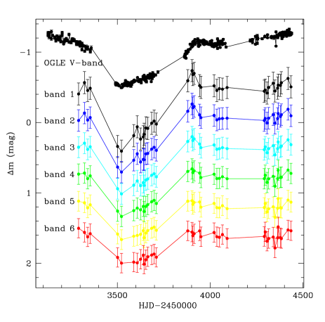
Based on this method, we could identify strong variations in the exponent $\alpha_{\nu}$ and intensity $f_{0}$ in the spectra of quasar images A and B. This indicates that the amplitude of the variations are significantly higher in the blue than in the red part of the spectra. In order to study in more detail these chromatic fluctuations of the continuum, we define six wavelength ranges, that we will use as photometric bands. The bands all have the same width and cover the whole wavelength range between 1500 and 3000 Å measured in the source frame, see Table 2. For each of these bands we compute the $\Delta m$ lightcurve by integrating the continuum power-law in the corresponding wavelength range. We give the corresponding AB magnitudes of the four quasar images in Table Microlensing variability in the gravitationally lensed quasar QSO 2237$+$0305 $\equiv$ the Einstein Cross . By subtracting the magnitude of image B from that of image A, we obtain six 39-epoch lightcurves, as displayed in Fig. 1. We immediately see that the lightcurves for the redder bands (e.g. band #6) vary less that the bluer ones (e.g. band #1).

Figure 1: The difference lightcurve $\Delta m$ between quasar images A and B measured in different wavelength bands. For clarity we shift the curves along the vertical direction. The binned OGLE observations with 181 data points measured in the V-band (Udalski et al., 2006). From our 39-epoch spectrophotometric monitoring, we compute the difference lightcurves of the continuum integrated in the six bands defined in Table 2.

Table 3: Macro-lensing parameters for images A and B from Kochanek (2004)

Image	$\kappa$	$\gamma$	$\mu_{macro}$
A	0.394	0.395	4.735
B	0.375	0.390	4.192

3 Microlensing Simulations

In order to simulate the microlensing effects, we have to choose a macro-model for the lensing galaxy. Many models have been proposed for the Einstein Cross (see for instance the summary in Table 2 of Wyithe et al., 2002). We choose the macro-model proposed by Kochanek (2004). The surface density $\kappa$, the shear $\gamma$, and the corresponding macro-magnifications $\mu_{macro}$ are given in Table 3. The convergence $\kappa$ is usually separated into a compact matter distribution $\kappa_{\star}$ and a smooth matter distribution $\kappa_{c}$ composed of gas and dark matter. However, as the quasar images are located within the bulge of the lensing galaxy, we do not expect a strong contribution from the smooth matter (Kochanek et al., 2007), so we neglect $\kappa_{c}$, which amounts to assuming the entire surface mass density is in stars (i.e. $\kappa=\kappa_{\star}$).

The next step is to define the mass distribution of the microlenses. Earlier investigations of microlensing have led to the conclusion that the magnification probability distribution is not very sensitive to the mass function of the microlenses (e.g. Wambsganss, 1992; Lewis & Irwin, 1995; Wyithe & Turner, 2001; Congdon et al., 2007), but that it depends on the mean microlens mass $\langle M\rangle$, which sets the parameter scales, such as the Einstein radius. The determination of $\langle M\rangle$ is not trivial because of the degeneracies existing between $\langle M\rangle$, the effective transverse velocity, and the source size. Several studies succeeded in getting an estimate of $\langle M\rangle$, and currently favor $\langle M\rangle\simeq 0.1\leavevmode\nobreak\ M_{\odot}$ (e.g. Wambsganss et al., 1990b; Lewis & Irwin, 1996). We will assume this value for all the microlenses distributed in the lens plane. This value is also consistent with the mean mass found by the MACHO collaboration who studied microlensing from objects located towards the bulge of the Milky Way (Alcock et al., 1997). See also Wyithe et al. (2000b), who give a summary of the determinations of microlens masses in other galaxies.

The masses of the microlenses sets the Einstein radius $r_{E}$. For QSO 2237$+$0305, the Einstein radius projects in the source plane as

$$r_{E}=D_{s}\leavevmode\nobreak\ \sqrt{\frac{4\mathrm{G}\langle M\rangle}{\mathrm{c}^{2}}\,\frac{D_{ls}}{D_{s}D_{l}}}=5.77\times 10^{16}\leavevmode\nobreak\ \langle M/0.1M_{\odot}\rangle^{1/2}\leavevmode\nobreak\ \textrm{cm.}$$

Having defined $\kappa$, $\gamma$ and the mass of the microlenses, we can go one step further in our simulations, and start generating large magnification patterns for the two quasar images A and B. We do this using the inverse ray-shooting method (Wambsganss, 1990; Wambsganss et al., 1990a). For each image, we shoot approximately $10^{11}$ rays from the observer through the lens plane back to the source plane, where the rays are collected in a $10,000$ by $10,000$ pixels array, corresponding to $100$ by $100$ Einstein radii.

In order to study a sample of different source sizes, the magnification patterns are convolved with a set of source profiles. Microlensing-induced flux variations are relatively insensitive to the source profile, but they depend on its characteristic size. Mortonson et al. (2005) showed that the half-light radius is the most important quantity for controlling the shape of microlensing light curves, whereas the source profile is less important. For simplicity we choose a Gaussian profile for the surface brightness, and we define the size of the source as the Full Width at Half Maximum (FWHM), which is twice as large as the half-light radius, and 2.35 greater than the Gaussian width $\sigma$.

The relative size of source with respect to the Einstein radius controls the smoothing of the magnification pattern. Very large source sizes (i.e. larger than $4\leavevmode\nobreak\ r_{E}$) produce magnification patterns that are so strongly smoothed, that they are unable to account for the amplitude (i.e. higher than $1$ mag) of the flux variations seen in the OGLE lightcurves. Hence, as was shown in previous studies (e.g. Wyithe et al., 2000a; Yonehara, 2001), we can safely rule out continuum source sizes larger than $4\leavevmode\nobreak\ r_{E}$. On the other hand, very small source sizes (i.e. smaller than $0.01\leavevmode\nobreak\ r_{E}$) give very moderately smoothed magnification patterns, which lead to sharp magnification events that are not observed in the OGLE lightcurves. The lower bound found in that way for the source size is $0.01\leavevmode\nobreak\ r_{E}$ (e.g. Kochanek, 2004; Anguita et al., 2008).

In the present study, we vary the FWHM of the Gaussian profile from 1 to 400 pixels, which corresponds to 0.01 $r_{E}$ and 4.00 $r_{E}$, respectively. We consider 45 different source sizes between these two extreme values. They are 1, 2, 4, 6, 8, 10, 12, 14, 16, 18, 20, 22, 24, 26, 28, 30, 35, 40, 45, 50, 55, 60, 65, 70, 75, 80, 85, 90, 95, 100, 120, 140, 160, 180, 200, 220, 240, 260, 280, 300, 320, 340, 360, 380, and 400 pixels.

4 Microlensing simulations fitting the OGLE data

Our simulations are conducted following the method described in Kochanek (2004). This technique is based on a Bayesian analysis, that determines the probability distributions for the physical parameters of interest by comparing trial lightcurves with the observed data. Because we want to infer probability distributions, we need to simulate a large number of these trial lightcurves in order to obtain a statistically significant sample. Thus, for each of our 45 source sizes, we simulate 10,000 light curves for both quasar images A and B by tracing source trajectories across the corresponding magnification patterns. We extract the pixel counts along the positions of the trajectory using bi-linear interpolation and we convert them into magnitudes. We subtract the simulated lightcurve of image B from that of image A, and obtain a total of $4.5\times 10^{5}$ difference lightcurves (10,000 for 45 different source sizes). Eventually, we want to compare this large library of simulated difference lightcurves to the $\Delta m$ observed in the OGLE data, but before we do that, we specify some characteristics of the simulated source trajectories.

The simulated lightcurves are obtained from source trajectories across the magnification patterns, and these trajectories are characterized by parameters of two kinds: physical and trajectory parameters. The physical parameters are the local magnification tensor $\kappa$ and $\gamma$, the mass $\langle M\rangle$ of the microlenses, the size $R_{s}$ of the source, the effective transverse velocity $V$ of the source, and the magnitude offset $m_{0}$ between the two images due to a combination of the macro-magnification, long-term microlensing, and differential extinction between the images. Because the scales of the magnification patterns are defined in terms of Einstein radii, our computational variables for the source size and velocity are in fact the scaled source size $\hat{R}_{s}=R_{s}/\langle M/0.1\leavevmode\nobreak\ M_{\odot}\rangle^{1/2}$ and the scaled transverse velocity $\hat{V}=V/\langle M/0.1\leavevmode\nobreak\ M_{\odot}\rangle^{1/2}$. Following these definitions, $\hat{R}_{s}$ is the relative size of the source with respect to the Einstein radius, and $\hat{V}$ is the velocity with which the source is moving across the magnification pattern.

Each source trajectory is also defined by the trajectory parameters $(\theta,\mathbf{x}_{0,A},\mathbf{x}_{0,B})$, where $\theta$ is the direction angle, $\mathbf{x}_{0,A}$ are the coordinates of the starting point in the magnification pattern of image A, and $\mathbf{x}_{0,B}$ in the pattern of image B. The trajectory is constrained to have identical directions $\theta$ and velocities $V$ across the patterns of images A and B. The direction is set to be the same in both patterns because the shear direction between images A and B is approximately the same Witt & Mao (1994), and because we assume the motion of the source to be primarily due to the bulk motion of the lensing galaxy rather than to the individual motions of the stars. Kundić & Wambsganss (1993) and Wambsganss & Kundić (1995) show that the velocity dispersion of the stars can statistically be interpreted as a bulk velocity artificially increased by an efficiency factor $a\simeq 1.3$.

For each particular choice of the parameters, that we write $p=(\kappa,\gamma,\langle M\rangle,\hat{R}_{s},\hat{V},m_{0},\theta,\mathbf{x}_{0,A},\mathbf{x}_{0,B})$, we get one simulated difference lightcurve $\Delta m^{\prime}_{k}(p)$, that can be compared to the observed data $D=\Delta m_{k}$ by measuring the goodness of fit with a $\chi^{2}$ statistic

$$\chi_{OGLE}^{2}(p)=\sum_{k=1}^{n_{obs}}\left(\frac{\Delta m_{k}-\Delta m_{k}^{\prime}(p)}{\sigma_{k}}\right)^{2}$$

where $\sigma_{k}$ are the uncertainties of the OGLE data, and $n_{obs}=181$ is the number of the binned OGLE data points. We determine the $\sigma_{k}$ from the photometric errors $\sigma_{OGLE}$ given by the OGLE project, from the standard deviation between the binned points $\sigma_{bin}$, and from the systematic error of the OGLE data $\sigma_{sys}$, with $\sigma_{k}^{2}=\sigma_{OGLE}^{2}+\sigma_{bin}^{2}+\sigma_{sys}^{2}$. We estimate the systematic error $\sigma_{sys}$ by carrying out a polynomial fit of the OGLE difference lightcurve $\Delta m_{k}$, using a polynomial of high enough order that the residuals are uncorrelated, i.e. such that the auto-correlation function of the residuals reduces to less than 0.5 within a separation of a few data points. We find that a polynomial on order 7 is sufficient, and $\sigma_{sys}=0.03$ mag.

By varying the parameters we construct our library of $4.5\times 10^{5}$ lightcurves. This produces an ensemble of models, which given the data and using Bayesian analysis (see Section 5) can infer the probability distributions for the parameters. The size of the magnification patterns is approximately one hundred times greater than the time scale of the observations multiplied by the effective velocity. Hence the available parameter space is huge, and it is relatively easy to find good fits to the data.

In our simulations we fix the values of $\kappa$, $\gamma$, and $\langle M\rangle$, and are left with the following set of variable parameters $p=(\hat{R}_{s},\hat{V},m_{0},\theta,\mathbf{x}_{0,A},\mathbf{x}_{0,B})$. The physical parameters that we want to investigate are the source size and the effective transverse velocity. The other parameters, i.e. $(m_{0},\theta,\mathbf{x}_{0,A},\mathbf{x}_{0,B})$, have no direct physical implications, and can be chosen arbitrarily. They are therefore called nuisance parameters. The influence of these parameters on the inferred probability distributions of $\hat{R}_{s}$ and $\hat{V}$ vanishes when using Bayesian analysis and a sufficiently large library of simulated lightcurves, as described in Section 5.

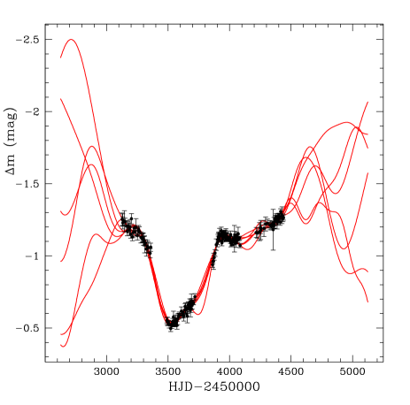
A first guess for the nuisance parameters $(m_{0},\theta,\mathbf{x}_{0,A},\mathbf{x}_{0,B})$ is chosen randomly following a uniform distribution. In the Bayesian analysis, lightcurves with low $\chi_{OGLE}^{2}$ values have relatively higher weights, and contribute more to the final probability distributions. An effective and fast method consists in searching for trajectories with low $\chi_{OGLE}^{2}$ values. To do this and hence minimize the necessary computing time, we follow the procedure described in Anguita et al. (2008), and optimize the seven parameters $(\hat{V},m_{0},\theta,\mathbf{x}_{0,A},\mathbf{x}_{0,B})$ with a $\chi^{2}$-based minimization algorithm using a Levenberg-Marquardt least squares routine in idl. We verify that this minimization technique still samples uniformly the whole magnification pattern. Finally we obtain a trajectory library containing $4.5\times 10^{5}$ trajectories (10,000 trajectories for 45 different source sizes) fitting the OGLE data. All the source trajectories have a reduced $\chi_{OGLE}^{2}/n_{dof}<10$, where $n_{dof}=345$ is the number of degrees of freedom, i.e. the number of observations minus the number of fitted parameters (here 7). Six examples of the simulated lightcurves are given in Fig. 2.

Figure 2: Examples of six simulated lightcurves fitting the observed OGLE difference lightcurve $\Delta m$ between quasar images A and B.

5 Bayesian analysis

In the previous section, we have described how we build our large library of trial lightcurves. We will now use these lightcurves to determine the probability distributions for the parameters $\hat{R}_{s}$ and $\hat{V}$ based on Bayesian analysis as described by Kochanek (2004). Following Bayes’ theorem the probability of the parameters $p=(\kappa,\gamma,\langle M\rangle,\hat{R}_{s},\hat{V},m_{0},\theta,\mathbf{x}_{0,A},\mathbf{x}_{0,B})$, given the data $D=\Delta m_{k}$, is

$$P(p|D)=\frac{P(D|p)\,P(p)}{P(D)}=\frac{L(D|p)}{N}\,P(p)$$

where $P(p)$ is the prior, $L(D|p)$ is the likelihood and $N$ is a normalization constant.

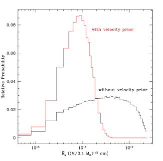
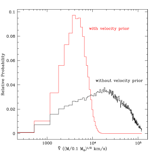
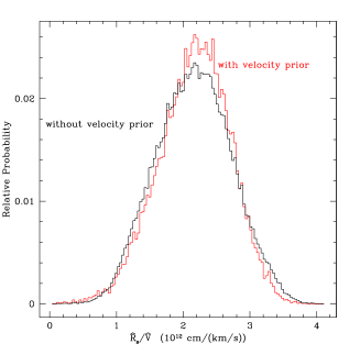
Figure 3: Left : The probability distributions for the FWHM $\hat{R}_{s}$ of the source, based on the OGLE data. We consider two cases, one with and another without the prior on the velocity. Center : Same as left panel, but for the effective transverse velocity $\hat{V}$. Right : The probability distributions for the ratio $\hat{R}_{s}/\hat{V}$.

We do not have any prior information either on the trajectory parameters $\theta,\mathbf{x}_{0,A},\mathbf{x}_{0,B}$ or on the magnitude offset $m_{0}$. Therefore we choose these parameters from a random and uniform distribution. This means that the corresponding priors $P(m_{0})$, $P(\theta)$, $P(\mathbf{x}_{0,A})$, and $P(\mathbf{x}_{0,B})$ are constant. We also assume that the parameters are independent, i.e. that

$$P(p)=P(\kappa)\,P(\gamma)\,P(\langle M\rangle)\,P(\hat{R}_{s})\,P(\hat{V})\,P(m_{0})\,P(\theta)\,P(\mathbf{x}_{0,A})\,P(\mathbf{x}_{0,B})\leavevmode\nobreak\ \textrm{.}$$

We define the relative likelihoods of the parameters $p$ based on the $\chi^{2}$ statistics. Usually, this is done following the standard approach for ensemble analysis (e.g., Sambridge, 1999), which uses the maximum likelihood estimator

$$L(D|p)=\exp\left(-\frac{1}{2}\,\chi^{2}(p)\right)\leavevmode\nobreak\ \textrm{.}$$

However, as noted by Kochanek (2004), using this standard estimator for the OGLE data works poorly because we are comparing the probabilities of completely different light curves rather than models related to each other by continuous changes of parameters. To circumvent this, we use the likelihood estimator proposed by Kochanek (2004)

$$L(D|p)=\Gamma\left[\frac{n_{dof}-2}{2},\frac{\chi^{2}(p)}{2}\right]$$

where $\Gamma$ is an incomplete Gamma function. Finally, all Bayesian parameter estimates have to be normalized by the requirement that the total probability is unity, i.e. $\int P(p|D)\leavevmode\nobreak\ \textrm{d}p=1$ and hence

$$N=\int L(D|p)\,P(p)\leavevmode\nobreak\ \textrm{d}p\leavevmode\nobreak\ \textrm{.}$$

In practice we sum the probabilities for our random sampling of trajectories, which is equivalent to using Monte Carlo integration methods to compute the integral over the ensemble of all possible trajectories. The sum over the random trajectories will converge to the true integral provided we consider a sufficiently large number of trajectories. The probability of a trajectory $j$ (defined by the set of parameters $p_{j}$) given the data $D$ is

$$P(p_{j}|D)=\frac{L(D|p_{j})\,P(\hat{R}_{s,j})\,P(\hat{V}_{j})}{\sum_{j=1}^{n}L(D|p_{j})\,P(\hat{R}_{s,j})\,P(\hat{V}_{j})}$$ (1)

where $n$ is the total number of trajectories in the library, and $P(\hat{R}_{s,j})$ and $P(\hat{V}_{j})$ are the priors on the source size and velocity, respectively. The priors on the other parameters are the same for all trajectories, and cancel out in the fraction above. The final probability distribution of the parameters are obtained by summing the probabilities $P(p_{j}|D)$ of all the trajectories $j$ of the library.

The prior $P(\hat{R}_{s,j})$ is required because we have not uniformly sampled the parameter space of the source size. We have to correct for this. The prior $P(\hat{R}_{s,j})$ is related to the density of trajectories as a function of $\hat{R}_{s,j}$ given our sampling of the source size in 45 different bins. Each bin contains 10,000 trajectories. Therefore, small bins have higher densities, and the corresponding $P(\hat{R}_{s,j})$ should be proportionally lower to compensate this effect, i.e. if the size of bin $b$ is $l_{b}$, and if $\hat{R}_{s,j}$ falls in this bin, then $P(\hat{R}_{s,j})\propto l_{b}$. Thus each bin has the same density of trajectories.

As already mentioned, there is a strong, essentially linear, correlation between $\hat{R}_{s}$ and $\hat{V}$, i.e. $\hat{R_{s}}\propto\hat{V}^{x}$ where $x\simeq 1$ (Kochanek, 2004). Furthermore, $\hat{R}_{s}$ and $\hat{V}$ are both defined as functions of $\langle M\rangle$, which imply degeneracies between $\langle M\rangle$, $\hat{V}$, and $\hat{R}_{s}$. However, since $R_{s}=\hat{R}_{s}\langle M/0.1M_{\odot}\rangle^{1/2}$ and $\langle M\rangle\propto(V/\hat{V})^{2}$, the physical size of the source $R_{s}\propto V\,\hat{V}^{x-1}\simeq V$ depends essentially on our estimate of the physical velocity $V$, and avoids the degeneracies between $\langle M\rangle$, $\hat{V}$, and $\hat{R}_{s}$.

Estimates of $V$ can be obtained from the observations of the motion of other galaxies or galaxy clusters (e.g. Benson et al., 2003), which show that peculiar velocities are typically not higher than $1,500$ km/s. In order to give a lower weight to trajectories having much higher velocities, we have to introduce a prior on the velocity. Previous studies have considered various priors (e.g. Kochanek, 2004; Gil-Merino et al., 2005). Some are more restrictive than others, but most of them have in common that they favor transverse velocities of $\sim 600$ km/s in the lens plane, which correspond to projected transverse velocities of $\sim 6,000$ km/s in the source plane of QSO 2237$+$0305 (Kayser et al., 1986).

The effective transverse velocity is the result of the relative motion between the source, the lens and the observer (Kayser et al., 1986), and is enhanced by a contribution from the velocity dispersion of the stars in the lensing galaxy (Kundić & Wambsganss, 1993; Wambsganss & Kundić, 1995). The problem is that we do not known the peculiar velocity of either the source, or the lens. The best we can do is to consider probability distributions for these unknown velocities, based on what we know from the peculiar motion of other galaxies (e.g. Mould et al., 1993; Benson et al., 2003). Kochanek (2004) shows that a good approximation for the probability distribution of the effective transverse velocity in the source-plane is

$$P(V)=\frac{V}{\bar{V}}\leavevmode\nobreak\ I_{0}\left[\frac{V\bar{V}}{\sigma^{2}}\right]\leavevmode\nobreak\ \exp\left(-\frac{V^{2}+\bar{V}^{2}}{2\sigma^{2}}\right)$$ (2)

where $I_{0}$ is a modified Bessel function, $\bar{V}\simeq 2500$ km/s is the mean velocity, and $\sigma\simeq 3500$ km/s is the total root mean square velocity obtained by considering all the different velocities contributing to the transverse effective velocity. In our analysis we assume $\langle M\rangle=0.1\leavevmode\nobreak\ M_{\odot}$, and we define the prior on the scaled velocity $\hat{V}$ as $P(\hat{V})=P(V)$.

Using Bayesian analysis, and considering both cases with and without velocity prior, we obtain the probability distributions of the source size $\hat{R}_{s}$, the effective transverse velocity $\hat{V}$, and the ratio $\hat{R}_{s}/\hat{V}$ plotted in Fig. 3. The results are given in Table 4.

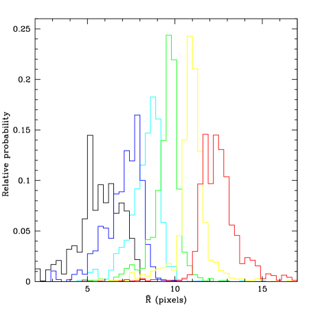
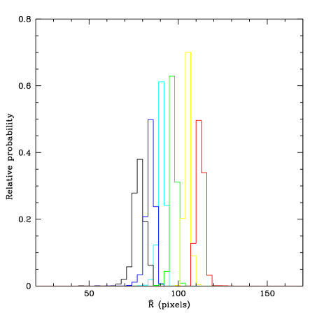
Figure 4: Top : The source FWHM ratio $R_{i}/R_{ref}=\hat{R}_{i}/\hat{R}_{ref}$ as a function of the wavelength ratio $\lambda_{i}/\lambda_{ref}$ obtained from the trajectories in the library having $\hat{R}_{s}=0.1\,r_{E}=10$ pixels (left) and $\hat{R}_{s}=1\,r_{E}=100$ pixels (right). The reference wavelength is $\lambda_{ref}=2125$ Å measured in the source frame. The error bars give the $1\sigma$ uncertainties. The solid line indicates the linear regression across the points. The dashed line shows the relation expected for the standard $R\propto\lambda^{4/3}$ scaling. Bottom : The corresponding probability distributions of the scaled source sizes $\hat{R}_{i}$ obtained in the six bands $i=1,2,...,6$, and using the same color code as in Fig. 1.

Table 4: Results from the microlensing simulations and Bayesian analysis applied to the OGLE data.

with velocity prior

$\qquad\hat{R}_{s}=\left(9.2^{+6.9}_{-5.8}\right)\times 10^{15}\,\langle M/0.1M_{\odot}\rangle^{1/2}$ cm $=\left(0.16^{+0.12}_{-0.10}\right)\leavevmode\nobreak\ r_{E}$

$\qquad\hat{V}=\left(3.9^{+3.0}_{-1.8}\right)\times 10^{3}\,\langle M/0.1M_{\odot}\rangle^{1/2}$ km/s

$\qquad\hat{R}_{s}/\hat{V}=\left(2.1\pm 0.5\right)\times 10^{12}$ cm/(km/s)

without velocity prior

$\qquad\hat{R}_{s}=\left(4.0^{+7.5}_{-3.5}\right)\times 10^{16}\,\langle M/0.1M_{\odot}\rangle^{1/2}$ cm $=\left(0.69^{+1.30}_{-0.60}\right)\leavevmode\nobreak\ r_{E}$

$\qquad\hat{V}=\left(1.8^{+2.8}_{-1.6}\right)\times 10^{4}\,\langle M/0.1M_{\odot}\rangle^{1/2}$ km/s

$\qquad\hat{R}_{s}/\hat{V}=\left(2.1\pm 0.6\right)\times 10^{12}$ cm/(km/s)

6 Energy profile of the quasar accretion disk

Accretion disk models for quasars generally make the assumption that the disk is optically thick and geometrically thin; both assumptions are required to cause efficient conversion of the gravitational potential energy of accreting matter into radiation (Pringle & Rees, 1972; Shakura & Sunyaev, 1973; Novikov & Thorne, 1973). Alternative models in which mass is lost in a wind (Kuncic & Bicknell, 2007), the disk accretes at greater than the Eddington limit and thus becomes geometrically thick, in which case advection or convection can dominate the radial heat transport (e.g. Abramowicz et al., 1988), or magnetic connections between the black hole and disk modify the rate of energy dissipation (Agol & Krolik, 2000).

The peak of the continuum emission in a typical quasar spectral energy distribution is in the ”Big Blue Bump”, and can be fitted well with a spectrum which scales as $F_{\nu}\propto\nu^{1/3}e^{h\nu/kT}$, with a characteristic temperature $T=7\times 10^{4}$ K (Krolik, 1998b). This is predicted by the standard thick accretion disk model in which $T\propto R^{-3/4}(1-(R_{in}/R)^{1/2})^{1/4}$, the functional form predicted by non-relativistic thin accretion disks with an inner edge $R_{in}$ at which the viscous stress disappears (relativity modifies this somewhat - Krolik, 1998a). At large radius $T\propto R^{-3/4}$, and the model predicts that the radiative flux $F$ (erg cm^-2 s^-1) at the surface of the disk at a radius $R$ is proportional to the energy production rate at that radius, resulting in $F\propto R^{-3}$. Since we are assuming a blackbody spectrum, $F\propto T^{4}$, and because the wavelength $\lambda$ of the peak of the black body spectrum is proportional to $T^{-1}$, most of the radiation at a given radius $R$ comes from near a radius

$$R\propto T^{-4/3}\propto\lambda^{4/3}\leavevmode\nobreak\ \textrm{.}$$

This defines the energy profile of the quasar, away from the inner edge of the disk, which is identical to the form obtained by Kochanek et al. (2007) from the standard thin accretion disk model of Shakura & Sunyaev (1973).

However, given that we are trying to test the accretion disk model, we allow the temperature to scale as a power-law with radius with arbitrary slope $T\propto R^{-\zeta}$ (Rauch & Blandford, 1991); this functional form is general enough to cover a variety of different alternatives to the standard accretion disk model.

There exist numerous models for quasar accretion disks in the literature. We can not consider all of them here, and we select only a few presenting an interesting variety. One particular model is motivated by the fact that the theoretical optical/UV continuum of a standard thin disk is $F_{\nu}\propto\nu^{1/3}$, which is inconsistent with $F_{\nu}\propto\nu^{-1}$ observed in many quasars. Hence, Gaskell (2008) suggests that the observed quasar spectra can be reproduced by accretion disks with a temperature gradient of $T\propto R^{-0.57}$ instead of $T\propto R^{-3/4}$. This implies

$$R\propto\lambda^{1.75}\leavevmode\nobreak\ \textrm{.}$$

Another model is proposed by Agol & Krolik (2000), and describes a disk which is powered by the spin of the central black hole. This changes the temperature profile to $T\propto r^{-7/8}$, and predicts

$$R\propto\lambda^{8/7}\leavevmode\nobreak\ \textrm{.}$$

The three models mentioned above all predict a power-law relation between the wavelength and the corresponding source size

$$R\propto\lambda^{\zeta}$$

with different values for the index $\zeta$. For two different radii $R$ and $R_{ref}$ emitting at the wavelengths $\lambda$ and $\lambda_{ref}$ respectively, we have

$$\frac{R}{R_{ref}}=\left(\frac{\lambda}{\lambda_{ref}}\right)^{\zeta}\qquad\Rightarrow\qquad\log\left(\frac{R}{R_{ref}}\right)=\zeta\leavevmode\nobreak\ \log\left(\frac{\lambda}{\lambda_{ref}}\right)\leavevmode\nobreak\ \textrm{.}$$

To distinguish between these different accretion disk models, we determine in the next section, which power-law is best compatible with our spectroscopic observations, and which of these models can be ruled out for QSO 2237$+$0305.

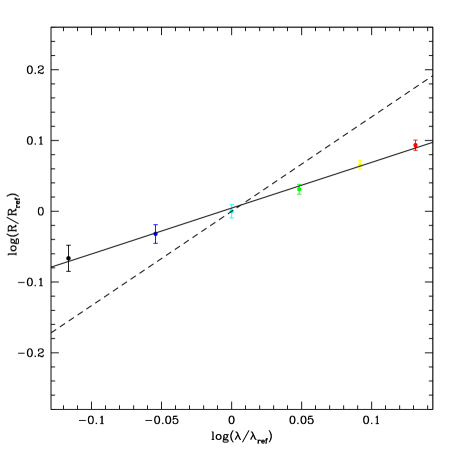
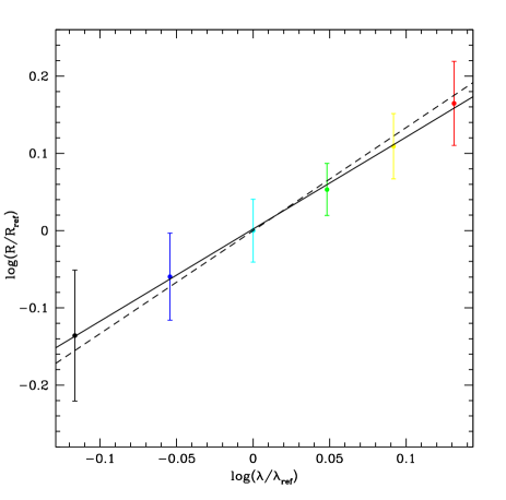
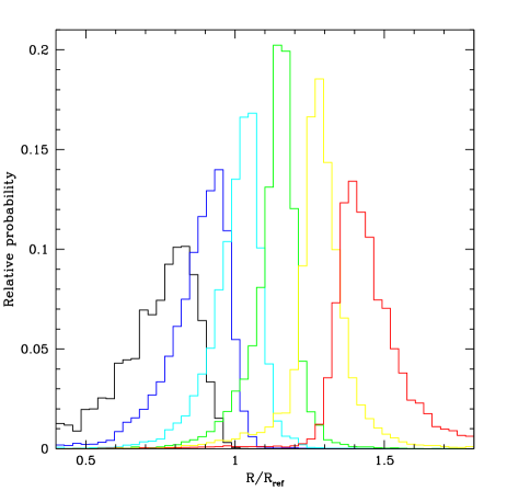
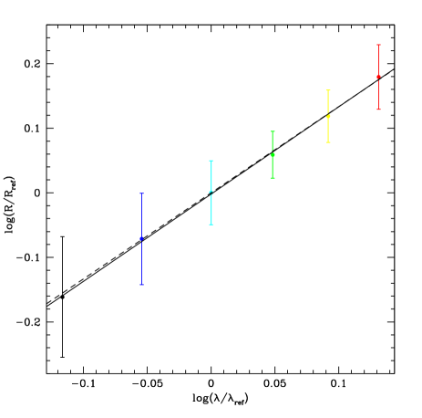
Figure 5: Left : The final energy profile obtained from the whole ensemble of source trajectories, including the prior on the velocity. The reference wavelength is $\lambda_{ref}=2125$ Å measured in the source frame. The error bars give the $1\sigma$ uncertainties. The solid line indicates the linear regression across the points. The dashed line shows the relation expected for the standard $R\propto\lambda^{4/3}$ scaling. Right : The corresponding probability distributions of the $R_{i}$ values obtained in the six bands $i=1,2,...,6$, and using the same color code as in Fig. 1.

7 Interpretation of the spectroscopic data

7.1 Method

We will now compare the theoretical energy profile with our observations. In the procedure described in the previous sections, we have built a library of simulated lightcurves by tracing a large number of source trajectories through the magnification patterns for various source sizes $\hat{R}_{s}$ in order to reproduce the OGLE V-band photometry $\Delta m$ of QSO 2237$+$0305. We use this ensemble of models as an input to extend our analysis to our spectroscopic observations. We consider the integrated lightcurves in the six color bands defined in Table 2 as shown in Fig. 1. For each band $i$, we have a lightcurve $\Delta m(\lambda_{i},t)$ with 39 epochs. The wavelength $\lambda_{i}$ is the central wavelength of band $i$ as defined in Table 2. We then determine which scaled source size $\hat{R}_{i}$ best reproduces the observed lightcurve in band $i$.

Each source trajectory $j$ in the library is defined by a set of the parameters $p_{j}=(\kappa_{j},\gamma_{j},\langle M\rangle_{j},\hat{R}_{s,j},\hat{V}_{j},m_{0,j},\theta_{j},\mathbf{x}_{0,A,j},\mathbf{x}_{0,B,j})$. For every trajectory $j$, we keep all these parameters fixed, except the source size $\hat{R}_{s,j}$, that we modify, i.e. we trace the same source trajectory in all the convolved magnification patterns. By doing this, we get the simulated difference lightcurve $\Delta m_{j}^{\prime}(t)$ corresponding to the 45 different source sizes defined in Section 3. We then interpolate the magnitude values of these extracted light curves to obtain continuous values for the source size. For every trajectory $j$, this defines a surface $\Delta m_{j}^{\prime}(\hat{R}_{s},t)$ in the three-dimensional space defined by $\hat{R}_{s}$, $t$ and $\Delta m$.

We use these $\Delta m_{j}^{\prime}(\hat{R}_{s},t)$ to interpret our spectroscopic data by determining which scaled source size $\hat{R}_{i}$ best reproduces the observed lighcurve $\Delta m(\lambda_{i},t)$ in band $i$. The size $\hat{R}_{i}$ is the value that minimizes the $\chi_{ij}^{2}$ between the spectrophotometric observations $\Delta m(\lambda_{i},t)$ and the simulated difference lightcurve $\Delta m_{j}^{\prime}(\hat{R}_{i},t)$. After this second fitting procedure, we update the relative likelihoods of the lightcurves

$$L(D|p_{j},i)=\Gamma\left[\frac{n_{dof}-2}{2},\frac{\chi_{OGLE}^{2}(p_{j})}{2}\right]\leavevmode\nobreak\ \times\leavevmode\nobreak\ \exp\left(-\frac{\chi_{ij}^{2}}{2}\right)$$

where $i$ refers to the considered band. In the fitting of the spectroscopic observations $\Delta m(\lambda_{i},t)$, we are comparing similar light curves, where only $\hat{R}_{i}$ is changing. This is a very different situation than when we were fitting the OGLE difference lightcurve and comparing simulations with very different parameters. Hence, we can use here the standard maximum likelihood estimator $\exp(-\chi_{ij}^{2}/2)$ to compute the likelihoods $L(D|p_{j},i)$. We run this procedure for all the simulated source trajectories $j$ in the library, and use these updated likelihoods to compute the final probability distribution for the parameters of interest, as described in section 5.

Figure 6: The power-law index $\zeta$ of the energy profile $R\propto\lambda^{\zeta}$ as a function of the scaled FWHM $\hat{R}_{s}$ of the source. The points are obtained from the subsamples of trajectories with given $\hat{R}_{s}$ fitting the OGLE data and including the prior on the velocity. The horizontal solid red lines indicate the index $\zeta$ and its $1\sigma$ deviation obtained by considering the whole library of trajectories and including the velocity prior. The dashed lines show the expected indices for the three indicated accretion-disk models.

7.2 Results

For each band $i$, we compute the probability distribution of the source-size ratio $\hat{R}_{i}/\hat{R}_{ref}$ following the Bayesian analysis described in Section 5 using equation (1). The reference radius $\hat{R}_{ref}$ at the reference wavelength $\lambda_{ref}$ can be chosen arbitrarily, and we simply define the middle band #3 as our reference. The scaling between $R_{s}$ and $\hat{R}_{s}$ is independent of the considered wavelength and $R_{i}/R_{ref}=\hat{R}_{i}/\hat{R}_{ref}$. Thus, the ratio $R_{i}/R_{ref}$ is not expected to depend on the assumed microlens mass $\langle M\rangle$. We plot the ratio $R_{i}/R_{ref}$ against the corresponding wavelength ratio $\lambda_{i}/\lambda_{ref}$, and determine the slope of the energy profile by fitting a power law

$$R\propto\lambda^{\zeta}\leavevmode\nobreak\ \textrm{.}$$

We do this for the entire library of source trajectories, but also individually for every subsample of the library with the same initial source size $\hat{R}_{s}$ used to fit the OGLE data. The resulting index $\zeta$ is plotted as a function of $\hat{R}_{s}$ in Fig. 6. We give two examples of energy profiles in Fig. 4 derived from subsamples of trajectories: one having $\hat{R}_{s}=0.1\,r_{E}=10$ pixels and another with $\hat{R}_{s}=1\,r_{E}=100$ pixels. The final energy profile obtained from the whole sample of source trajectories is shown in Fig. 5, given in Table 5, and yields $\zeta=1.2\pm 0.3$ when adding the velocity prior. Without this prior we get a flatter energy profile with $\zeta=1.1\pm 0.3$.

Table 5: The relative size $R_{i}/R_{ref}$ obtained for the six photometric bands, including the velocity prior.

Band	$\lambda_{c}$ [Å]	$R_{i}/R_{ref}$
1	1625	0.73 $\pm$ 0.14
2	1875	0.87 $\pm$ 0.11
3	2125	1.00 $\pm$ 0.09
4	2375	1.13 $\pm$ 0.09
5	2625	1.29 $\pm$ 0.13
6	2875	1.46 $\pm$ 0.18

8 Discussion

From the results of our microlensing simulations, we can extract several interesting facts. First, the source FWHM $\hat{R}_{s}=\left(0.16^{+0.12}_{-0.10}\right)\leavevmode\nobreak\ r_{E}$ we derive from the fitting of the OGLE data (including the prior on the velocity) is well compatible with the upper limit of $0.98\leavevmode\nobreak\ r_{E}$ given by Yonehara (2001). Our result is also in good agreement with the FWHM derived by Anguita et al. (2008), $\hat{R}_{s}=(0.06\pm 0.01)\leavevmode\nobreak\ r_{E}$, and by Kochanek (2004), $\hat{R}_{s}=\left(0.20^{+0.19}_{-0.12}\right)\leavevmode\nobreak\ r_{E}$. The differences between these estimates of $\hat{R}_{s}$ can have two origins. First, as mentioned by Kochanek (2004), the probability distributions obtained for the parameters depend on the choice of the period of observations. If the considered period is very active in terms of microlensing, the simulations will favor high transverse velocities and/or small source sizes. Second, the choice of the velocity prior has a strong effect on the derived source size. As we observe in Fig. 3, there is a strong correlation between the scaled source size $\hat{R}_{s}$ and the scaled effective transverse velocity $\hat{V}$. Independently of the velocity prior considered, we find that the source size is directly proportional to the transverse velocity, with the relation $\hat{R}_{s}/\hat{V}=\left(2.1\pm 0.6\right)\times 10^{12}$ cm/(km/s). This is in excellent agreement with Kochanek (2004), who also finds $\hat{R}_{s}/\hat{V}=2.1\times 10^{12}$ cm/(km/s), where $R_{s}$ is expressed as the FWHM. This defines the time scale of the observed microlensing-induced fluctuations, which is given by the half-light radius divided by the effective transverse velocity, i.e. $0.5\leavevmode\nobreak\ \hat{R}_{s}/\hat{V}=4.0\pm 1.0$ months, and which is independent of microlens masses or velocity priors.

The strong correlation between $\hat{R}_{s}$ and $\hat{V}$ (Kochanek, 2004) implies that the choice of the velocity prior and the selection of the observation period can both bias our estimate of the source size. The microlensing activity during our observations was not as important as during the periods studied by Kochanek (2004) and Anguita et al. (2008). Furthermore, Anguita et al. (2008) considered a shorter observation period, and used the velocity prior of Gil-Merino et al. (2005), which is more constraining towards high velocities (hence favoring smaller source sizes) than the one we considered in the present study. This explains, why our derived $\hat{R}_{s}$ is slightly larger. One possible solution to minimize the bias induced by the selection of the observation period is to consider the longest possible lightcurves, but this has the evident drawback of dramatically increasing the computing effort, making the problem rapidly intractable. However, as discussed in the following, the estimate of the source size has only a limited effect on our determination of the energy profile.

From our library of simulated source trajectories fitting the OGLE data, we extend our analysis to our spectroscopic data, and determine the energy profile $R\propto\lambda^{\zeta}$ of the quasar accretion disk. When we consider the whole library and include the prior on the velocity, we get $\zeta=1.2\pm 0.3$, which is in good agreement with the model of Agol & Krolik (2000) and with the $\zeta=4/3$ index expected from the standard accretion disk model. It is less compatible (at $1\sigma$) with the accretion disk model of Gaskell (2008). Our findings are also in good agreement with Anguita et al. (2008), who obtain $\left(6400\leavevmode\nobreak\ \textrm{\AA}/4700\leavevmode\nobreak\ \textrm{\AA}\right)^{\zeta}=1.45^{+0.90}_{-0.25}$, which yields a power-law index $\zeta=1.2^{+2.0}_{-0.6}$. Without the velocity prior, we get a lower value $\zeta=1.1\pm 0.3$, which is still compatible with $\zeta=8/7$ and $4/3$, but less with the model of Gaskell (2008). This is expected because, without the prior, large sources gain relatively more importance in the Bayesian analysis, and favor flatter energy profile, as shown in Fig. 6. However, as discussed earlier, large source sizes imply unlikely high transverse velocities, and hence a much more reliable result is obtained when including the velocity prior.

We observe that our result for the $R\propto\lambda^{\zeta}$ scaling is not very sensitive on the velocity prior with respect to other parameters. For instance, we know that the source size $\hat{R}_{s}$ is extremely sensitive to such a prior, and can vary over orders of magnitudes if the considered transverse velocity does. On the contrary, the index $\zeta$ varies only by a few percent, even if the considered velocities are modified by orders of magnitude. Hence, and independently of the determination of $\hat{V}$ and $\hat{R}_{s}$, the chromatic variations between two images of a lensed quasar are extremely efficient in constraining the relative sizes of different regions of the accretion disk. This is further confirmed by the fact that Anguita et al. (2008) obtain a value for $\zeta$ which is in good agreement with ours, even though they derive a slightly smaller source size.

The influence of the initial value of the parameter $\hat{R}_{s}$ (chosen to fit the OGLE data) on the resulting energy profile of the accretion disk is obvious in Fig. 6. Sources having sizes in the range $0.06\leq\hat{R}_{s}\leq 0.2\,r_{E}$ are in good agreement with the $\zeta=8/7$ and $4/3$ scalings, while larger sources give flatter energy profiles, and smaller sources steeper profiles. The same behavior is observed, when we omit the velocity prior.

9 Conclusion

We present the continuation of our spectrophotometric monitoring of QSO 2237$+$0305 conducted at the Very Large Telescope of the European Southern Observatory, which extends over more than three years from October 2004 to December 2007. Our program provides the spectra of the four lensed images at 43 epochs. Analysis of these data show that the continuum and the broad line region of the background quasar are microlensed, and that images A and B are particularly affected. In this paper, we focus on the observed variations in the continuum of the spectra of these two images, and use them to constrain the energy profile of the quasar.

We build microlensing magnification patterns with the inverse ray-shooting method (Wambsganss, 1990; Wambsganss et al., 1990a), and convolve them with different source sizes. We trace source trajectories through these convolved patterns and fit the observed OGLE difference lightcurve between image A and image B. Combining these simulations with Bayesian analysis following the method proposed by Kochanek (2004), we infer probability distributions for the effective transverse velocity $V$, and the source size $R_{s}$ of the quasar. Our results are compatible with previous studies.

Besides the OGLE broad-band photometry, we analyze the data of our spectroscopic monitoring and derived the corresponding difference lightcurves in six different photometric bands. Each band is 250 Å wide and together the bands cover the wavelength range between 1500 and 3000 Å (measured in the rest frame of the source). We compute the difference lightcurves between images A and B in these six bands, and observe that, as expected from the microlensing of an accretion disk, bands at bluer wavelengths exhibit stronger flux variations than bands at redder wavelengths.

Based on these chromatic variations and using the ensemble of the microlensing simulations that are fitting the OGLE data, we determine the relative sizes of the regions of the accretion disk emitting in the six photometric bands, i.e. we derive the energy profile of the accretion disk. We find that this profile follows a power-law $R\propto\lambda^{\zeta}$ with $\zeta=1.2\pm 0.3$, which is in good agreement with the standard thin accretion disk model of Shakura & Sunyaev (1973) ($\zeta=4/3$) and with the model of Agol & Krolik (2000) ($\zeta=8/7$), where the disk is powered by the spin of the central black hole. Our result is less compatible with the model of Gaskell (2008), which predicts a steeper energy profile ($\zeta=1.75$). Our result compares well with that obtained by Poindexter et al. (2008) from multi-band photometry of the lensed quasar HE 1104$-$1805. They analyzed microlensing lightcurves in eleven bands from the optical to the mid-infrared, and found that both the size and energy profile $\zeta=1.64^{+0.46}_{-0.56}$ (i.e. their $\beta^{-1}$) of the quasar accretion disk are consistent with the standard disk model of Shakura & Sunyaev (1973).

We observe that the determination of the power law-index is almost independent of the velocity prior used, whereas the determination of the scaled source size $\hat{R}_{s}$ is directly proportional to the scaled effective transverse velocity $\hat{V}$. This is easily explained by the fact that the scaling between $R_{s}$ and $\hat{R}_{s}$ is independent of the considered wavelength, and hence $R_{i}/R_{ref}=\hat{R}_{i}/\hat{R}_{ref}$. As a consequence, the determination of relative source sizes, and hence of the energy profile, is not expected to depend on the assumed microlens mass $\langle M\rangle$.

Quasar microlensing is hence able to resolve structures of accretion disks on scales reaching $0.1$ micro-arcsecond, which is more than $10,000$ times better than the resolution reached by today’s best telescopes. Finally, we should mention several recent studies that compare microlensing in the X-ray and optical domain, and that further demonstrate the efficiency of microlensing in probing the inner parts of quasars. For instance, Morgan et al. (2008) analyze the lightcurves of the lensed quasar PG 1115$+$080, and find that the effective radius of the X-ray emission is $1.3^{+1.1}_{-0.5}$ dex smaller than that of the optical emission, with the X-ray emission generated near the inner edge of the accretion disk while the optical emission comes from scales slightly larger than those expected for a standard thin disk. Pooley et al. (2008) observe extreme microlensing-induced (de-) magnification of the lensed images of PG 1115$+$080, and conclude that about 90% of the matter in the lensing galaxy is in smoothly distributed (dark) material and only about 10% is in compact (stellar) objects. Another example is given by Chartas et al. (2008), who combine X-ray and optical data of HE 1104$-$1805, and reveal that the X-ray emitting region is compact with a half-light radius smaller than six gravitational radius, i.e. smaller than $2\times 10^{15}$ cm, thus placing significant constraints on active galactic nuclei models.

References

• Abramowicz et al. (1988) Abramowicz, M. A., Czerny, B., Lasota, J. P., & Szuszkiewicz, E. 1988, ApJ, 332, 646
• Agol & Krolik (2000) Agol, E. & Krolik, J. H. 2000, ApJ, 528, 161
• Alcalde et al. (2002) Alcalde, D., Mediavilla, E., Moreau, O., et al. 2002, ApJ, 572, 729
• Alcock et al. (1997) Alcock, C., Allsman, R. A., Alves, D., et al. 1997, ApJ, 479, 119
• Anguita et al. (2008) Anguita, T., Schmidt, R. W., Turner, E. L., et al. 2008, A&A, 480, 327
• Benson et al. (2003) Benson, B. A., Church, S. E., Ade, P. A. R., et al. 2003, ApJ, 592, 674
• Chartas et al. (2008) Chartas, G., Kochanek, C. S., Dai, X., Poindexter, S., & Garmire, G. 2008, astro-ph/0805.4492
• Congdon et al. (2007) Congdon, A. B., Keeton, C. R., & Osmer, S. J. 2007, MNRAS, 376, 263
• Corrigan et al. (1991) Corrigan, R. T., Irwin, M. J., Arnaud, J., et al. 1991, AJ, 102, 34
• Eigenbrod et al. (2008) Eigenbrod, A., Courbin, F., Sluse, D., Meylan, G., & Agol, E. 2008, A&A, 480, 647
• Gaskell (2008) Gaskell, C. M. 2008, in Revista Mexicana de Astronomia y Astrofisica Conference Series, Vol. 32, Revista Mexicana de Astronomia y Astrofisica Conference Series, 1–11
• Gil-Merino et al. (2005) Gil-Merino, R., Wambsganss, J., Goicoechea, L. J., & Lewis, G. F. 2005, A&A, 432, 83
• Huchra et al. (1985) Huchra, J., Gorenstein, M., Kent, S., et al. 1985, AJ, 90, 691
• Kayser et al. (1986) Kayser, R., Refsdal, S., & Stabell, R. 1986, A&A, 166, 36
• Kochanek (2004) Kochanek, C. S. 2004, ApJ, 605, 58
• Kochanek et al. (2007) Kochanek, C. S., Dai, X., Morgan, C., Morgan, N., & Poindexter, S. C. G. 2007, in Astronomical Society of the Pacific Conference Series, Vol. 371, Statistical Challenges in Modern Astronomy IV, ed. G. J. Babu & E. D. Feigelson, 43
• Krolik (1998a) Krolik, J. H. 1998a, Active Galactic Nuclei: From the Central Black Hole to the Galactic Environment (Princeton University Press)
• Krolik (1998b) Krolik, J. H. 1998b, in Non-linear Phenomena in Accretion Disks around Black Holes, 134–147
• Kuncic & Bicknell (2007) Kuncic, Z. & Bicknell, G. V. 2007, Ap&SS, 311, 127
• Kundić & Wambsganss (1993) Kundić, T. & Wambsganss, J. 1993, ApJ, 404, 455
• Lewis & Irwin (1995) Lewis, G. F. & Irwin, M. J. 1995, MNRAS, 276, 103
• Lewis & Irwin (1996) Lewis, G. F. & Irwin, M. J. 1996, MNRAS, 283, 225
• Lynden-Bell (1969) Lynden-Bell, D. 1969, Nature, 223, 690
• Morgan et al. (2008) Morgan, C. W., Kochanek, C. S., Dai, X., Morgan, N. D., & Falco, E. E. 2008, astro-ph/0802.1210
• Morgan et al. (2007) Morgan, C. W., Kochanek, C. S., Morgan, N. D., & Falco, E. E. 2007, astro-ph/0707.0305
• Mortonson et al. (2005) Mortonson, M. J., Schechter, P. L., & Wambsganss, J. 2005, ApJ, 628, 594
• Mould et al. (1993) Mould, J. R., Akeson, R. L., Bothun, G. D., et al. 1993, ApJ, 409, 14
• Novikov & Thorne (1973) Novikov, I. D. & Thorne, K. S. 1973, in Black Holes (Les Astres Occlus), 343–450
• Ostensen et al. (1996) Ostensen, R., Refsdal, S., Stabell, R., et al. 1996, A&A, 309, 59
• Poindexter et al. (2008) Poindexter, S., Morgan, N., & Kochanek, C. S. 2008, ApJ, 673, 34
• Pooley et al. (2007) Pooley, D., Blackburne, J. A., Rappaport, S., & Schechter, P. L. 2007, ApJ, 661, 19
• Pooley et al. (2008) Pooley, D., Rappaport, S., Blackburne, J., et al. 2008, astro-ph/0808.3299
• Pringle & Rees (1972) Pringle, J. E. & Rees, M. J. 1972, A&A, 21, 1
• Rauch & Blandford (1991) Rauch, K. P. & Blandford, R. D. 1991, ApJ, 381, L39
• Rix et al. (1992) Rix, H.-W., Schneider, D. P., & Bahcall, J. N. 1992, AJ, 104, 959
• Sambridge (1999) Sambridge, M. 1999, Geophysical Journal International, 138, 727
• Schmidt et al. (2002) Schmidt, R. W., Kundić, T., Pen, U.-L., et al. 2002, A&A, 392, 773
• Schneider et al. (1988) Schneider, D. P., Turner, E. L., Gunn, J. E., et al. 1988, AJ, 95, 1619
• Shakura & Sunyaev (1973) Shakura, N. I. & Sunyaev, R. A. 1973, A&A, 24, 337
• Shields (1978) Shields, G. A. 1978, Nature, 272, 706
• Udalski et al. (2006) Udalski, A., Szymanski, M. K., Kubiak, M., et al. 2006, Acta Astronomica, 56, 293
• Wambsganss (1990) Wambsganss, J. 1990, PhD thesis, Thesis Ludwig-Maximilians-Univ., Munich (Germany, F. R.). Fakultät für Physik., (1990)
• Wambsganss (1992) Wambsganss, J. 1992, ApJ, 386, 19
• Wambsganss & Kundić (1995) Wambsganss, J. & Kundić, T. 1995, ApJ, 450, 19
• Wambsganss & Paczyński (1991) Wambsganss, J. & Paczyński, B. 1991, AJ, 102, 864
• Wambsganss & Paczyński (1994) Wambsganss, J. & Paczyński, B. 1994, AJ, 108, 1156
• Wambsganss et al. (1990a) Wambsganss, J., Paczyński, B., & Katz, N. 1990a, ApJ, 352, 407
• Wambsganss et al. (1990b) Wambsganss, J., Paczyński, B., & Schneider, P. 1990b, ApJ, 358, L33
• Witt & Mao (1994) Witt, H. J. & Mao, S. 1994, ApJ, 429, 66
• Woźniak et al. (2000a) Woźniak, P. R., Alard, C., Udalski, A., et al. 2000a, ApJ, 529, 88
• Woźniak et al. (2000b) Woźniak, P. R., Udalski, A., Szymański, M., et al. 2000b, ApJ, 540, L65
• Wyithe et al. (2002) Wyithe, J. S. B., Agol, E., & Fluke, C. J. 2002, MNRAS, 331, 1041
• Wyithe & Turner (2001) Wyithe, J. S. B. & Turner, E. L. 2001, MNRAS, 320, 21
• Wyithe et al. (2000a) Wyithe, J. S. B., Webster, R. L., & Turner, E. L. 2000a, MNRAS, 318, 762
• Wyithe et al. (2000b) Wyithe, J. S. B., Webster, R. L., & Turner, E. L. 2000b, MNRAS, 315, 51
• Yonehara (2001) Yonehara, A. 2001, ApJ, 548, L127
\LT@array
[x]cccccccc Continuum integrated AB magnitudes in the six photometric bands defined in Table 2.
ID HJD band 1 (mag) band 2 (mag) band 3 (mag) band 4 (mag) band 5 (mag) band 6 (mag)
\endfirsthead
Continued.
\endhead\endfoot
Image A
1 3292 17.97±0.05plus-or-minus17.970.0517.97\pm 0.05 17.81±0.05plus-or-minus17.810.0517.81\pm 0.05 17.67±0.05plus-or-minus17.670.0517.67\pm 0.05 17.54±0.06plus-or-minus17.540.0617.54\pm 0.06 17.43±0.06plus-or-minus17.430.0617.43\pm 0.06 17.33±0.05plus-or-minus17.330.0517.33\pm 0.05
2 3324 18.02±0.05plus-or-minus18.020.0518.02\pm 0.05 17.87±0.04plus-or-minus17.870.0417.87\pm 0.04 17.73±0.04plus-or-minus17.730.0417.73\pm 0.04 17.61±0.05plus-or-minus17.610.0517.61\pm 0.05 17.50±0.05plus-or-minus17.500.0517.50\pm 0.05 17.40±0.04plus-or-minus17.400.0417.40\pm 0.04
3 3341 18.02±0.06plus-or-minus18.020.0618.02\pm 0.06 17.85±0.05plus-or-minus17.850.0517.85\pm 0.05 17.71±0.05plus-or-minus17.710.0517.71\pm 0.05 17.59±0.06plus-or-minus17.590.0617.59\pm 0.06 17.47±0.06plus-or-minus17.470.0617.47\pm 0.06 17.37±0.05plus-or-minus17.370.0517.37\pm 0.05
4 3355 17.98±0.08plus-or-minus17.980.0817.98\pm 0.08 17.83±0.08plus-or-minus17.830.0817.83\pm 0.08 17.69±0.07plus-or-minus17.690.0717.69\pm 0.07 17.57±0.08plus-or-minus17.570.0817.57\pm 0.08 17.47±0.08plus-or-minus17.470.0817.47\pm 0.08 17.37±0.08plus-or-minus17.370.0817.37\pm 0.08
5 3502 18.07±0.04plus-or-minus18.070.0418.07\pm 0.04 17.88±0.04plus-or-minus17.880.0417.88\pm 0.04 17.72±0.04plus-or-minus17.720.0417.72\pm 0.04 17.57±0.04plus-or-minus17.570.0417.57\pm 0.04 17.44±0.04plus-or-minus17.440.0417.44\pm 0.04 17.33±0.04plus-or-minus17.330.0417.33\pm 0.04
6 3523 18.16±0.05plus-or-minus18.160.0518.16\pm 0.05 17.97±0.05plus-or-minus17.970.0517.97\pm 0.05 17.80±0.04plus-or-minus17.800.0417.80\pm 0.04 17.64±0.05plus-or-minus17.640.0517.64\pm 0.05 17.51±0.05plus-or-minus17.510.0517.51\pm 0.05 17.39±0.04plus-or-minus17.390.0417.39\pm 0.04
7 3553 18.23±0.04plus-or-minus18.230.0418.23\pm 0.04 18.03±0.04plus-or-minus18.030.0418.03\pm 0.04 17.85±0.03plus-or-minus17.850.0317.85\pm 0.03 17.69±0.04plus-or-minus17.690.0417.69\pm 0.04 17.55±0.04plus-or-minus17.550.0417.55\pm 0.04 17.42±0.03plus-or-minus17.420.0317.42\pm 0.03
8 3566 18.16±0.06plus-or-minus18.160.0618.16\pm 0.06 17.96±0.06plus-or-minus17.960.0617.96\pm 0.06 17.79±0.05plus-or-minus17.790.0517.79\pm 0.05 17.63±0.06plus-or-minus17.630.0617.63\pm 0.06 17.49±0.06plus-or-minus17.490.0617.49\pm 0.06 17.37±0.05plus-or-minus17.370.0517.37\pm 0.05
9 3589 18.24±0.04plus-or-minus18.240.0418.24\pm 0.04 18.04±0.04plus-or-minus18.040.0418.04\pm 0.04 17.87±0.03plus-or-minus17.870.0317.87\pm 0.03 17.71±0.04plus-or-minus17.710.0417.71\pm 0.04 17.57±0.04plus-or-minus17.570.0417.57\pm 0.04 17.45±0.03plus-or-minus17.450.0317.45\pm 0.03
10 3598 18.24±0.06plus-or-minus18.240.0618.24\pm 0.06 18.03±0.06plus-or-minus18.030.0618.03\pm 0.06 17.84±0.06plus-or-minus17.840.0617.84\pm 0.06 17.68±0.06plus-or-minus17.680.0617.68\pm 0.06 17.53±0.06plus-or-minus17.530.0617.53\pm 0.06 17.39±0.06plus-or-minus17.390.0617.39\pm 0.06
11 3608 18.21±0.03plus-or-minus18.210.0318.21\pm 0.03 18.02±0.03plus-or-minus18.020.0318.02\pm 0.03 17.86±0.03plus-or-minus17.860.0317.86\pm 0.03 17.71±0.04plus-or-minus17.710.0417.71\pm 0.04 17.58±0.04plus-or-minus17.580.0417.58\pm 0.04 17.47±0.03plus-or-minus17.470.0317.47\pm 0.03
12 3626 18.21±0.05plus-or-minus18.210.0518.21\pm 0.05 18.01±0.05plus-or-minus18.010.0518.01\pm 0.05 17.83±0.04plus-or-minus17.830.0417.83\pm 0.04 17.68±0.05plus-or-minus17.680.0517.68\pm 0.05 17.54±0.05plus-or-minus17.540.0517.54\pm 0.05 17.42±0.04plus-or-minus17.420.0417.42\pm 0.04
13 3641 18.11±0.05plus-or-minus18.110.0518.11\pm 0.05 17.90±0.05plus-or-minus17.900.0517.90\pm 0.05 17.73±0.05plus-or-minus17.730.0517.73\pm 0.05 17.57±0.05plus-or-minus17.570.0517.57\pm 0.05 17.43±0.05plus-or-minus17.430.0517.43\pm 0.05 17.30±0.05plus-or-minus17.300.0517.30\pm 0.05
14 3645 18.08±0.05plus-or-minus18.080.0518.08\pm 0.05 17.91±0.05plus-or-minus17.910.0517.91\pm 0.05 17.77±0.05plus-or-minus17.770.0517.77\pm 0.05 17.64±0.05plus-or-minus17.640.0517.64\pm 0.05 17.52±0.05plus-or-minus17.520.0517.52\pm 0.05 17.42±0.05plus-or-minus17.420.0517.42\pm 0.05
15 3655 18.10±0.04plus-or-minus18.100.0418.10\pm 0.04 17.92±0.04plus-or-minus17.920.0417.92\pm 0.04 17.77±0.03plus-or-minus17.770.0317.77\pm 0.03 17.63±0.04plus-or-minus17.630.0417.63\pm 0.04 17.51±0.04plus-or-minus17.510.0417.51\pm 0.04 17.39±0.03plus-or-minus17.390.0317.39\pm 0.03
16 3665 18.10±0.04plus-or-minus18.100.0418.10\pm 0.04 17.92±0.04plus-or-minus17.920.0417.92\pm 0.04 17.75±0.04plus-or-minus17.750.0417.75\pm 0.04 17.61±0.04plus-or-minus17.610.0417.61\pm 0.04 17.48±0.04plus-or-minus17.480.0417.48\pm 0.04 17.36±0.04plus-or-minus17.360.0417.36\pm 0.04
17 3686 17.93±0.06plus-or-minus17.930.0617.93\pm 0.06 17.77±0.06plus-or-minus17.770.0617.77\pm 0.06 17.63±0.06plus-or-minus17.630.0617.63\pm 0.06 17.50±0.07plus-or-minus17.500.0717.50\pm 0.07 17.39±0.07plus-or-minus17.390.0717.39\pm 0.07 17.28±0.06plus-or-minus17.280.0617.28\pm 0.06
18 3699 17.94±0.04plus-or-minus17.940.0417.94\pm 0.04 17.78±0.04plus-or-minus17.780.0417.78\pm 0.04 17.64±0.04plus-or-minus17.640.0417.64\pm 0.04 17.51±0.04plus-or-minus17.510.0417.51\pm 0.04 17.40±0.04plus-or-minus17.400.0417.40\pm 0.04 17.30±0.04plus-or-minus17.300.0417.30\pm 0.04
19 3711 17.88±0.07plus-or-minus17.880.0717.88\pm 0.07 17.71±0.07plus-or-minus17.710.0717.71\pm 0.07 17.57±0.07plus-or-minus17.570.0717.57\pm 0.07 17.44±0.07plus-or-minus17.440.0717.44\pm 0.07 17.33±0.07plus-or-minus17.330.0717.33\pm 0.07 17.22±0.07plus-or-minus17.220.0717.22\pm 0.07
20 3880 17.58±0.04plus-or-minus17.580.0417.58\pm 0.04 17.47±0.05plus-or-minus17.470.0517.47\pm 0.05 17.36±0.04plus-or-minus17.360.0417.36\pm 0.04 17.26±0.05plus-or-minus17.260.0517.26\pm 0.05 17.17±0.05plus-or-minus17.170.0517.17\pm 0.05 17.08±0.04plus-or-minus17.080.0417.08\pm 0.04
21 3903 17.50±0.03plus-or-minus17.500.0317.50\pm 0.03 17.40±0.04plus-or-minus17.400.0417.40\pm 0.04 17.30±0.04plus-or-minus17.300.0417.30\pm 0.04 17.20±0.04plus-or-minus17.200.0417.20\pm 0.04 17.12±0.04plus-or-minus17.120.0417.12\pm 0.04 17.04±0.04plus-or-minus17.040.0417.04\pm 0.04
22 3907 17.50±0.03plus-or-minus17.500.0317.50\pm 0.03 17.39±0.03plus-or-minus17.390.0317.39\pm 0.03 17.28±0.03plus-or-minus17.280.0317.28\pm 0.03 17.19±0.04plus-or-minus17.190.0417.19\pm 0.04 17.10±0.04plus-or-minus17.100.0417.10\pm 0.04 17.02±0.03plus-or-minus17.020.0317.02\pm 0.03
23 3914 17.51±0.02plus-or-minus17.510.0217.51\pm 0.02 17.41±0.03plus-or-minus17.410.0317.41\pm 0.03 17.30±0.03plus-or-minus17.300.0317.30\pm 0.03 17.21±0.03plus-or-minus17.210.0317.21\pm 0.03 17.12±0.03plus-or-minus17.120.0317.12\pm 0.03 17.04±0.03plus-or-minus17.040.0317.04\pm 0.03
24 3944 17.53±0.04plus-or-minus17.530.0417.53\pm 0.04 17.39±0.04plus-or-minus17.390.0417.39\pm 0.04 17.27±0.04plus-or-minus17.270.0417.27\pm 0.04 17.16±0.04plus-or-minus17.160.0417.16\pm 0.04 17.07±0.04plus-or-minus17.070.0417.07\pm 0.04 16.98±0.04plus-or-minus16.980.0416.98\pm 0.04
25 3951 17.51±0.03plus-or-minus17.510.0317.51\pm 0.03 17.39±0.03plus-or-minus17.390.0317.39\pm 0.03 17.28±0.03plus-or-minus17.280.0317.28\pm 0.03 17.18±0.03plus-or-minus17.180.0317.18\pm 0.03 17.10±0.04plus-or-minus17.100.0417.10\pm 0.04 17.02±0.03plus-or-minus17.020.0317.02\pm 0.03
26 4022 17.54±0.03plus-or-minus17.540.0317.54\pm 0.03 17.41±0.04plus-or-minus17.410.0417.41\pm 0.04 17.29±0.03plus-or-minus17.290.0317.29\pm 0.03 17.19±0.04plus-or-minus17.190.0417.19\pm 0.04 17.09±0.04plus-or-minus17.090.0417.09\pm 0.04 17.01±0.03plus-or-minus17.010.0317.01\pm 0.03
27 4037 17.53±0.03plus-or-minus17.530.0317.53\pm 0.03 17.40±0.03plus-or-minus17.400.0317.40\pm 0.03 17.29±0.03plus-or-minus17.290.0317.29\pm 0.03 17.19±0.04plus-or-minus17.190.0417.19\pm 0.04 17.09±0.04plus-or-minus17.090.0417.09\pm 0.04 17.01±0.03plus-or-minus17.010.0317.01\pm 0.03
28 4050 17.44±0.04plus-or-minus17.440.0417.44\pm 0.04 17.33±0.04plus-or-minus17.330.0417.33\pm 0.04 17.23±0.04plus-or-minus17.230.0417.23\pm 0.04 17.14±0.04plus-or-minus17.140.0417.14\pm 0.04 17.06±0.04plus-or-minus17.060.0417.06\pm 0.04 16.99±0.04plus-or-minus16.990.0416.99\pm 0.04
29 4067 17.41±0.05plus-or-minus17.410.0517.41\pm 0.05 17.29±0.05plus-or-minus17.290.0517.29\pm 0.05 17.19±0.05plus-or-minus17.190.0517.19\pm 0.05 17.09±0.05plus-or-minus17.090.0517.09\pm 0.05 17.01±0.05plus-or-minus17.010.0517.01\pm 0.05 16.93±0.05plus-or-minus16.930.0516.93\pm 0.05
31 4092 17.40±0.04plus-or-minus17.400.0417.40\pm 0.04 17.30±0.05plus-or-minus17.300.0517.30\pm 0.05 17.20±0.04plus-or-minus17.200.0417.20\pm 0.04 17.12±0.05plus-or-minus17.120.0517.12\pm 0.05 17.05±0.05plus-or-minus17.050.0517.05\pm 0.05 16.99±0.04plus-or-minus16.990.0416.99\pm 0.04
32 4292 17.51±0.03plus-or-minus17.510.0317.51\pm 0.03 17.36±0.03plus-or-minus17.360.0317.36\pm 0.03 17.22±0.03plus-or-minus17.220.0317.22\pm 0.03 17.10±0.03plus-or-minus17.100.0317.10\pm 0.03 16.99±0.03plus-or-minus16.990.0316.99\pm 0.03 16.89±0.03plus-or-minus16.890.0316.89\pm 0.03
33 4297 17.49±0.03plus-or-minus17.490.0317.49\pm 0.03 17.33±0.03plus-or-minus17.330.0317.33\pm 0.03 17.19±0.03plus-or-minus17.190.0317.19\pm 0.03 17.06±0.03plus-or-minus17.060.0317.06\pm 0.03 16.95±0.03plus-or-minus16.950.0316.95\pm 0.03 16.85±0.03plus-or-minus16.850.0316.85\pm 0.03
34 4307 17.42±0.03plus-or-minus17.420.0317.42\pm 0.03 17.31±0.03plus-or-minus17.310.0317.31\pm 0.03 17.21±0.03plus-or-minus17.210.0317.21\pm 0.03 17.12±0.04plus-or-minus17.120.0417.12\pm 0.04 17.04±0.04plus-or-minus17.040.0417.04\pm 0.04 16.97±0.03plus-or-minus16.970.0316.97\pm 0.03
35 4316 17.46±0.03plus-or-minus17.460.0317.46\pm 0.03 17.34±0.03plus-or-minus17.340.0317.34\pm 0.03 17.23±0.03plus-or-minus17.230.0317.23\pm 0.03 17.13±0.03plus-or-minus17.130.0317.13\pm 0.03 17.04±0.03plus-or-minus17.040.0317.04\pm 0.03 16.97±0.03plus-or-minus16.970.0316.97\pm 0.03
36 4340 17.43±0.04plus-or-minus17.430.0417.43\pm 0.04 17.29±0.04plus-or-minus17.290.0417.29\pm 0.04 17.17±0.04plus-or-minus17.170.0417.17\pm 0.04 17.06±0.04plus-or-minus17.060.0417.06\pm 0.04 16.97±0.04plus-or-minus16.970.0416.97\pm 0.04 16.88±0.04plus-or-minus16.880.0416.88\pm 0.04
37 4350 17.44±0.03plus-or-minus17.440.0317.44\pm 0.03 17.36±0.03plus-or-minus17.360.0317.36\pm 0.03 17.29±0.03plus-or-minus17.290.0317.29\pm 0.03 17.23±0.03plus-or-minus17.230.0317.23\pm 0.03 17.18±0.03plus-or-minus17.180.0317.18\pm 0.03 17.13±0.03plus-or-minus17.130.0317.13\pm 0.03
38 4364 17.40±0.03plus-or-minus17.400.0317.40\pm 0.03 17.28±0.03plus-or-minus17.280.0317.28\pm 0.03 17.18±0.03plus-or-minus17.180.0317.18\pm 0.03 17.09±0.03plus-or-minus17.090.0317.09\pm 0.03 17.00±0.03plus-or-minus17.000.0317.00\pm 0.03 16.93±0.03plus-or-minus16.930.0316.93\pm 0.03
39 4367 17.35±0.06plus-or-minus17.350.0617.35\pm 0.06 17.23±0.06plus-or-minus17.230.0617.23\pm 0.06 17.11±0.06plus-or-minus17.110.0617.11\pm 0.06 17.02±0.07plus-or-minus17.020.0717.02\pm 0.07 16.93±0.07plus-or-minus16.930.0716.93\pm 0.07 16.85±0.06plus-or-minus16.850.0616.85\pm 0.06
40 4379 17.39±0.02plus-or-minus17.390.0217.39\pm 0.02 17.26±0.02plus-or-minus17.260.0217.26\pm 0.02 17.15±0.02plus-or-minus17.150.0217.15\pm 0.02 17.05±0.03plus-or-minus17.050.0317.05\pm 0.03 16.96±0.03plus-or-minus16.960.0316.96\pm 0.03 16.87±0.02plus-or-minus16.870.0216.87\pm 0.02
41 4384 17.41±0.03plus-or-minus17.410.0317.41\pm 0.03 17.29±0.03plus-or-minus17.290.0317.29\pm 0.03 17.20±0.03plus-or-minus17.200.0317.20\pm 0.03 17.11±0.04plus-or-minus17.110.0417.11\pm 0.04 17.03±0.04plus-or-minus17.030.0417.03\pm 0.04 16.96±0.03plus-or-minus16.960.0316.96\pm 0.03
42 4420 17.39±0.05plus-or-minus17.390.0517.39\pm 0.05 17.25±0.05plus-or-minus17.250.0517.25\pm 0.05 17.13±0.05plus-or-minus17.130.0517.13\pm 0.05 17.02±0.05plus-or-minus17.020.0517.02\pm 0.05 16.93±0.05plus-or-minus16.930.0516.93\pm 0.05 16.84±0.05plus-or-minus16.840.0516.84\pm 0.05
43 4436 17.39±0.03plus-or-minus17.390.0317.39\pm 0.03 17.23±0.04plus-or-minus17.230.0417.23\pm 0.04 17.09±0.03plus-or-minus17.090.0317.09\pm 0.03 16.96±0.04plus-or-minus16.960.0416.96\pm 0.04 16.85±0.04plus-or-minus16.850.0416.85\pm 0.04 16.75±0.03plus-or-minus16.750.0316.75\pm 0.03
Image B
1 3293 19.08±0.12plus-or-minus19.080.1219.08\pm 0.12 18.94±0.12plus-or-minus18.940.1218.94\pm 0.12 18.82±0.11plus-or-minus18.820.1118.82\pm 0.11 18.71±0.13plus-or-minus18.710.1318.71\pm 0.13 18.62±0.13plus-or-minus18.620.1318.62\pm 0.13 18.53±0.11plus-or-minus18.530.1118.53\pm 0.11
2 3324 19.29±0.10plus-or-minus19.290.1019.29\pm 0.10 19.11±0.09plus-or-minus19.110.0919.11\pm 0.09 18.94±0.08plus-or-minus18.940.0818.94\pm 0.08 18.79±0.09plus-or-minus18.790.0918.79\pm 0.09 18.66±0.09plus-or-minus18.660.0918.66\pm 0.09 18.54±0.09plus-or-minus18.540.0918.54\pm 0.09
3 3341 19.18±0.14plus-or-minus19.180.1419.18\pm 0.14 18.99±0.14plus-or-minus18.990.1418.99\pm 0.14 18.83±0.12plus-or-minus18.830.1218.83\pm 0.12 18.69±0.14plus-or-minus18.690.1418.69\pm 0.14 18.57±0.14plus-or-minus18.570.1418.57\pm 0.14 18.45±0.13plus-or-minus18.450.1318.45\pm 0.13
4 3356 19.17±0.14plus-or-minus19.170.1419.17\pm 0.14 19.00±0.14plus-or-minus19.000.1419.00\pm 0.14 18.85±0.13plus-or-minus18.850.1318.85\pm 0.13 18.72±0.14plus-or-minus18.720.1418.72\pm 0.14 18.60±0.14plus-or-minus18.600.1418.60\pm 0.14 18.49±0.13plus-or-minus18.490.1318.49\pm 0.13
5 3503 18.43±0.05plus-or-minus18.430.0518.43\pm 0.05 18.35±0.05plus-or-minus18.350.0518.35\pm 0.05 18.28±0.04plus-or-minus18.280.0418.28\pm 0.04 18.22±0.05plus-or-minus18.220.0518.22\pm 0.05 18.17±0.05plus-or-minus18.170.0518.17\pm 0.05 18.12±0.05plus-or-minus18.120.0518.12\pm 0.05
6 3523 18.46±0.06plus-or-minus18.460.0618.46\pm 0.06 18.36±0.06plus-or-minus18.360.0618.36\pm 0.06 18.28±0.06plus-or-minus18.280.0618.28\pm 0.06 18.21±0.06plus-or-minus18.210.0618.21\pm 0.06 18.15±0.06plus-or-minus18.150.0618.15\pm 0.06 18.09±0.06plus-or-minus18.090.0618.09\pm 0.06
9 3589 18.76±0.05plus-or-minus18.760.0518.76\pm 0.05 18.61±0.06plus-or-minus18.610.0618.61\pm 0.06 18.48±0.05plus-or-minus18.480.0518.48\pm 0.05 18.37±0.06plus-or-minus18.370.0618.37\pm 0.06 18.26±0.06plus-or-minus18.260.0618.26\pm 0.06 18.17±0.05plus-or-minus18.170.0518.17\pm 0.05
11 3608 18.85±0.05plus-or-minus18.850.0518.85\pm 0.05 18.68±0.05plus-or-minus18.680.0518.68\pm 0.05 18.53±0.05plus-or-minus18.530.0518.53\pm 0.05 18.40±0.05plus-or-minus18.400.0518.40\pm 0.05 18.28±0.05plus-or-minus18.280.0518.28\pm 0.05 18.18±0.05plus-or-minus18.180.0518.18\pm 0.05
12 3626 18.67±0.06plus-or-minus18.670.0618.67\pm 0.06 18.55±0.06plus-or-minus18.550.0618.55\pm 0.06 18.44±0.06plus-or-minus18.440.0618.44\pm 0.06 18.35±0.07plus-or-minus18.350.0718.35\pm 0.07 18.26±0.07plus-or-minus18.260.0718.26\pm 0.07 18.18±0.06plus-or-minus18.180.0618.18\pm 0.06
13 3641 18.61±0.06plus-or-minus18.610.0618.61\pm 0.06 18.48±0.07plus-or-minus18.480.0718.48\pm 0.07 18.38±0.06plus-or-minus18.380.0618.38\pm 0.06 18.28±0.07plus-or-minus18.280.0718.28\pm 0.07 18.20±0.07plus-or-minus18.200.0718.20\pm 0.07 18.12±0.06plus-or-minus18.120.0618.12\pm 0.06
14 3645 18.62±0.07plus-or-minus18.620.0718.62\pm 0.07 18.49±0.08plus-or-minus18.490.0818.49\pm 0.08 18.38±0.07plus-or-minus18.380.0718.38\pm 0.07 18.28±0.08plus-or-minus18.280.0818.28\pm 0.08 18.19±0.08plus-or-minus18.190.0818.19\pm 0.08 18.11±0.07plus-or-minus18.110.0718.11\pm 0.07
15 3655 18.73±0.06plus-or-minus18.730.0618.73\pm 0.06 18.58±0.06plus-or-minus18.580.0618.58\pm 0.06 18.45±0.06plus-or-minus18.450.0618.45\pm 0.06 18.34±0.06plus-or-minus18.340.0618.34\pm 0.06 18.24±0.06plus-or-minus18.240.0618.24\pm 0.06 18.15±0.06plus-or-minus18.150.0618.15\pm 0.06
16 3665 18.72±0.06plus-or-minus18.720.0618.72\pm 0.06 18.58±0.06plus-or-minus18.580.0618.58\pm 0.06 18.46±0.06plus-or-minus18.460.0618.46\pm 0.06 18.35±0.07plus-or-minus18.350.0718.35\pm 0.07 18.25±0.07plus-or-minus18.250.0718.25\pm 0.07 18.16±0.06plus-or-minus18.160.0618.16\pm 0.06
17 3686 18.63±0.10plus-or-minus18.630.1018.63\pm 0.10 18.50±0.10plus-or-minus18.500.1018.50\pm 0.10 18.38±0.09plus-or-minus18.380.0918.38\pm 0.09 18.28±0.10plus-or-minus18.280.1018.28\pm 0.10 18.19±0.10plus-or-minus18.190.1018.19\pm 0.10 18.10±0.09plus-or-minus18.100.0918.10\pm 0.09
18 3699 18.66±0.08plus-or-minus18.660.0818.66\pm 0.08 18.53±0.08plus-or-minus18.530.0818.53\pm 0.08 18.41±0.08plus-or-minus18.410.0818.41\pm 0.08 18.31±0.09plus-or-minus18.310.0918.31\pm 0.09 18.22±0.09plus-or-minus18.220.0918.22\pm 0.09 18.13±0.08plus-or-minus18.130.0818.13\pm 0.08
19 3711 18.56±0.11plus-or-minus18.560.1118.56\pm 0.11 18.42±0.11plus-or-minus18.420.1118.42\pm 0.11 18.30±0.10plus-or-minus18.300.1018.30\pm 0.10 18.20±0.11plus-or-minus18.200.1118.20\pm 0.11 18.10±0.11plus-or-minus18.100.1118.10\pm 0.11 18.01±0.10plus-or-minus18.010.1018.01\pm 0.10
20 3880 18.83±0.12plus-or-minus18.830.1218.83\pm 0.12 18.74±0.13plus-or-minus18.740.1318.74\pm 0.13 18.59±0.12plus-or-minus18.590.1218.59\pm 0.12 18.47±0.14plus-or-minus18.470.1418.47\pm 0.14 18.35±0.14plus-or-minus18.350.1418.35\pm 0.14 18.25±0.12plus-or-minus18.250.1218.25\pm 0.12
21 3903 18.89±0.07plus-or-minus18.890.0718.89\pm 0.07 18.77±0.07plus-or-minus18.770.0718.77\pm 0.07 18.60±0.07plus-or-minus18.600.0718.60\pm 0.07 18.45±0.08plus-or-minus18.450.0818.45\pm 0.08 18.31±0.08plus-or-minus18.310.0818.31\pm 0.08 18.19±0.07plus-or-minus18.190.0718.19\pm 0.07
22 3907 18.83±0.06plus-or-minus18.830.0618.83\pm 0.06 18.71±0.07plus-or-minus18.710.0718.71\pm 0.07 18.53±0.07plus-or-minus18.530.0718.53\pm 0.07 18.38±0.07plus-or-minus18.380.0718.38\pm 0.07 18.25±0.07plus-or-minus18.250.0718.25\pm 0.07 18.12±0.07plus-or-minus18.120.0718.12\pm 0.07
23 3914 18.86±0.05plus-or-minus18.860.0518.86\pm 0.05 18.74±0.06plus-or-minus18.740.0618.74\pm 0.06 18.57±0.05plus-or-minus18.570.0518.57\pm 0.05 18.42±0.06plus-or-minus18.420.0618.42\pm 0.06 18.29±0.06plus-or-minus18.290.0618.29\pm 0.06 18.17±0.05plus-or-minus18.170.0518.17\pm 0.05
24 3944 18.76±0.07plus-or-minus18.760.0718.76\pm 0.07 18.60±0.07plus-or-minus18.600.0718.60\pm 0.07 18.47±0.06plus-or-minus18.470.0618.47\pm 0.06 18.35±0.07plus-or-minus18.350.0718.35\pm 0.07 18.24±0.07plus-or-minus18.240.0718.24\pm 0.07 18.15±0.06plus-or-minus18.150.0618.15\pm 0.06
25 3951 18.72±0.06plus-or-minus18.720.0618.72\pm 0.06 18.56±0.06plus-or-minus18.560.0618.56\pm 0.06 18.43±0.06plus-or-minus18.430.0618.43\pm 0.06 18.31±0.06plus-or-minus18.310.0618.31\pm 0.06 18.20±0.06plus-or-minus18.200.0618.20\pm 0.06 18.10±0.06plus-or-minus18.100.0618.10\pm 0.06
26 4022 18.76±0.06plus-or-minus18.760.0618.76\pm 0.06 18.61±0.06plus-or-minus18.610.0618.61\pm 0.06 18.48±0.05plus-or-minus18.480.0518.48\pm 0.05 18.36±0.06plus-or-minus18.360.0618.36\pm 0.06 18.25±0.06plus-or-minus18.250.0618.25\pm 0.06 18.15±0.05plus-or-minus18.150.0518.15\pm 0.05
27 4037 18.69±0.05plus-or-minus18.690.0518.69\pm 0.05 18.54±0.05plus-or-minus18.540.0518.54\pm 0.05 18.41±0.05plus-or-minus18.410.0518.41\pm 0.05 18.29±0.05plus-or-minus18.290.0518.29\pm 0.05 18.19±0.05plus-or-minus18.190.0518.19\pm 0.05 18.09±0.05plus-or-minus18.090.0518.09\pm 0.05
28 4050 18.63±0.09plus-or-minus18.630.0918.63\pm 0.09 18.49±0.09plus-or-minus18.490.0918.49\pm 0.09 18.36±0.08plus-or-minus18.360.0818.36\pm 0.08 18.25±0.09plus-or-minus18.250.0918.25\pm 0.09 18.15±0.09plus-or-minus18.150.0918.15\pm 0.09 18.06±0.08plus-or-minus18.060.0818.06\pm 0.08
29 4067 18.59±0.12plus-or-minus18.590.1218.59\pm 0.12 18.46±0.12plus-or-minus18.460.1218.46\pm 0.12 18.34±0.12plus-or-minus18.340.1218.34\pm 0.12 18.23±0.12plus-or-minus18.230.1218.23\pm 0.12 18.13±0.12plus-or-minus18.130.1218.13\pm 0.12 18.05±0.12plus-or-minus18.050.1218.05\pm 0.12
30 4089 18.57±0.14plus-or-minus18.570.1418.57\pm 0.14 18.45±0.14plus-or-minus18.450.1418.45\pm 0.14 18.34±0.13plus-or-minus18.340.1318.34\pm 0.13 18.25±0.14plus-or-minus18.250.1418.25\pm 0.14 18.16±0.14plus-or-minus18.160.1418.16\pm 0.14 18.08±0.13plus-or-minus18.080.1318.08\pm 0.13
31 4093 18.60±0.10plus-or-minus18.600.1018.60\pm 0.10 18.46±0.10plus-or-minus18.460.1018.46\pm 0.10 18.34±0.09plus-or-minus18.340.0918.34\pm 0.09 18.23±0.10plus-or-minus18.230.1018.23\pm 0.10 18.13±0.10plus-or-minus18.130.1018.13\pm 0.10 18.05±0.09plus-or-minus18.050.0918.05\pm 0.09
32 4292 18.66±0.06plus-or-minus18.660.0618.66\pm 0.06 18.49±0.07plus-or-minus18.490.0718.49\pm 0.07 18.34±0.06plus-or-minus18.340.0618.34\pm 0.06 18.21±0.07plus-or-minus18.210.0718.21\pm 0.07 18.09±0.06plus-or-minus18.090.0618.09\pm 0.06 17.98±0.06plus-or-minus17.980.0617.98\pm 0.06
33 4297 18.66±0.07plus-or-minus18.660.0718.66\pm 0.07 18.49±0.07plus-or-minus18.490.0718.49\pm 0.07 18.35±0.06plus-or-minus18.350.0618.35\pm 0.06 18.22±0.07plus-or-minus18.220.0718.22\pm 0.07 18.11±0.07plus-or-minus18.110.0718.11\pm 0.07 18.00±0.06plus-or-minus18.000.0618.00\pm 0.06
34 4307 18.54±0.09plus-or-minus18.540.0918.54\pm 0.09 18.40±0.09plus-or-minus18.400.0918.40\pm 0.09 18.28±0.08plus-or-minus18.280.0818.28\pm 0.08 18.17±0.09plus-or-minus18.170.0918.17\pm 0.09 18.08±0.09plus-or-minus18.080.0918.08\pm 0.09 17.99±0.08plus-or-minus17.990.0817.99\pm 0.08
35 4316 18.66±0.08plus-or-minus18.660.0818.66\pm 0.08 18.50±0.09plus-or-minus18.500.0918.50\pm 0.09 18.36±0.08plus-or-minus18.360.0818.36\pm 0.08 18.24±0.09plus-or-minus18.240.0918.24\pm 0.09 18.12±0.09plus-or-minus18.120.0918.12\pm 0.09 18.02±0.08plus-or-minus18.020.0818.02\pm 0.08
36 4340 18.69±0.13plus-or-minus18.690.1318.69\pm 0.13 18.51±0.13plus-or-minus18.510.1318.51\pm 0.13 18.35±0.12plus-or-minus18.350.1218.35\pm 0.12 18.20±0.13plus-or-minus18.200.1318.20\pm 0.13 18.07±0.13plus-or-minus18.070.1318.07\pm 0.13 17.96±0.12plus-or-minus17.960.1217.96\pm 0.12
37 4350 18.59±0.08plus-or-minus18.590.0818.59\pm 0.08 18.46±0.08plus-or-minus18.460.0818.46\pm 0.08 18.34±0.08plus-or-minus18.340.0818.34\pm 0.08 18.23±0.08plus-or-minus18.230.0818.23\pm 0.08 18.14±0.08plus-or-minus18.140.0818.14\pm 0.08 18.05±0.08plus-or-minus18.050.0818.05\pm 0.08
38 4364 18.60±0.09plus-or-minus18.600.0918.60\pm 0.09 18.44±0.09plus-or-minus18.440.0918.44\pm 0.09 18.31±0.09plus-or-minus18.310.0918.31\pm 0.09 18.20±0.10plus-or-minus18.200.1018.20\pm 0.10 18.09±0.09plus-or-minus18.090.0918.09\pm 0.09 18.00±0.09plus-or-minus18.000.0918.00\pm 0.09
39 4367 18.59±0.16plus-or-minus18.590.1618.59\pm 0.16 18.46±0.17plus-or-minus18.460.1718.46\pm 0.17 18.34±0.15plus-or-minus18.340.1518.34\pm 0.15 18.24±0.17plus-or-minus18.240.1718.24\pm 0.17 18.15±0.17plus-or-minus18.150.1718.15\pm 0.17 18.07±0.16plus-or-minus18.070.1618.07\pm 0.16
40 4379 18.62±0.05plus-or-minus18.620.0518.62\pm 0.05 18.45±0.06plus-or-minus18.450.0618.45\pm 0.06 18.30±0.05plus-or-minus18.300.0518.30\pm 0.05 18.17±0.06plus-or-minus18.170.0618.17\pm 0.06 18.05±0.06plus-or-minus18.050.0618.05\pm 0.06 17.94±0.05plus-or-minus17.940.0517.94\pm 0.05
41 4384 18.68±0.06plus-or-minus18.680.0618.68\pm 0.06 18.51±0.07plus-or-minus18.510.0718.51\pm 0.07 18.36±0.06plus-or-minus18.360.0618.36\pm 0.06 18.24±0.07plus-or-minus18.240.0718.24\pm 0.07 18.12±0.07plus-or-minus18.120.0718.12\pm 0.07 18.01±0.06plus-or-minus18.010.0618.01\pm 0.06
42 4421 18.72±0.09plus-or-minus18.720.0918.72\pm 0.09 18.54±0.09plus-or-minus18.540.0918.54\pm 0.09 18.39±0.08plus-or-minus18.390.0818.39\pm 0.08 18.25±0.09plus-or-minus18.250.0918.25\pm 0.09 18.13±0.09plus-or-minus18.130.0918.13\pm 0.09 18.02±0.08plus-or-minus18.020.0818.02\pm 0.08
43 4436 18.60±0.07plus-or-minus18.600.0718.60\pm 0.07 18.43±0.07plus-or-minus18.430.0718.43\pm 0.07 18.28±0.06plus-or-minus18.280.0618.28\pm 0.06 18.14±0.07plus-or-minus18.140.0718.14\pm 0.07 18.02±0.07plus-or-minus18.020.0718.02\pm 0.07 17.91±0.06plus-or-minus17.910.0617.91\pm 0.06
Image C
1 3293 19.08±0.11plus-or-minus19.080.1119.08\pm 0.11 18.92±0.12plus-or-minus18.920.1218.92\pm 0.12 18.78±0.11plus-or-minus18.780.1118.78\pm 0.11 18.65±0.13plus-or-minus18.650.1318.65\pm 0.13 18.54±0.13plus-or-minus18.540.1318.54\pm 0.13 18.44±0.11plus-or-minus18.440.1118.44\pm 0.11
2 3324 19.32±0.09plus-or-minus19.320.0919.32\pm 0.09 19.09±0.08plus-or-minus19.090.0819.09\pm 0.08 18.90±0.08plus-or-minus18.900.0818.90\pm 0.08 18.73±0.09plus-or-minus18.730.0918.73\pm 0.09 18.57±0.09plus-or-minus18.570.0918.57\pm 0.09 18.43±0.08plus-or-minus18.430.0818.43\pm 0.08
3 3341 19.22±0.14plus-or-minus19.220.1419.22\pm 0.14 19.01±0.14plus-or-minus19.010.1419.01\pm 0.14 18.82±0.13plus-or-minus18.820.1318.82\pm 0.13 18.65±0.14plus-or-minus18.650.1418.65\pm 0.14 18.50±0.14plus-or-minus18.500.1418.50\pm 0.14 18.37±0.12plus-or-minus18.370.1218.37\pm 0.12
4 3356 19.44±0.16plus-or-minus19.440.1619.44\pm 0.16 19.22±0.16plus-or-minus19.220.1619.22\pm 0.16 19.02±0.16plus-or-minus19.020.1619.02\pm 0.16 18.85±0.18plus-or-minus18.850.1818.85\pm 0.18 18.69±0.18plus-or-minus18.690.1818.69\pm 0.18 18.55±0.15plus-or-minus18.550.1518.55\pm 0.15
5 3503 19.28±0.08plus-or-minus19.280.0819.28\pm 0.08 19.09±0.08plus-or-minus19.090.0819.09\pm 0.08 18.93±0.08plus-or-minus18.930.0818.93\pm 0.08 18.79±0.09plus-or-minus18.790.0918.79\pm 0.09 18.66±0.08plus-or-minus18.660.0818.66\pm 0.08 18.54±0.08plus-or-minus18.540.0818.54\pm 0.08
6 3523 19.29±0.10plus-or-minus19.290.1019.29\pm 0.10 19.09±0.10plus-or-minus19.090.1019.09\pm 0.10 18.91±0.10plus-or-minus18.910.1018.91\pm 0.10 18.76±0.11plus-or-minus18.760.1118.76\pm 0.11 18.62±0.10plus-or-minus18.620.1018.62\pm 0.10 18.50±0.09plus-or-minus18.500.0918.50\pm 0.09
9 3589 19.46±0.09plus-or-minus19.460.0919.46\pm 0.09 19.23±0.09plus-or-minus19.230.0919.23\pm 0.09 19.02±0.08plus-or-minus19.020.0819.02\pm 0.08 18.83±0.09plus-or-minus18.830.0918.83\pm 0.09 18.67±0.09plus-or-minus18.670.0918.67\pm 0.09 18.52±0.08plus-or-minus18.520.0818.52\pm 0.08
11 3608 19.59±0.09plus-or-minus19.590.0919.59\pm 0.09 19.32±0.09plus-or-minus19.320.0919.32\pm 0.09 19.10±0.08plus-or-minus19.100.0819.10\pm 0.08 18.89±0.09plus-or-minus18.890.0918.89\pm 0.09 18.71±0.08plus-or-minus18.710.0818.71\pm 0.08 18.54±0.08plus-or-minus18.540.0818.54\pm 0.08
12 3626 19.38±0.10plus-or-minus19.380.1019.38\pm 0.10 19.17±0.11plus-or-minus19.170.1119.17\pm 0.11 18.99±0.10plus-or-minus18.990.1018.99\pm 0.10 18.83±0.11plus-or-minus18.830.1118.83\pm 0.11 18.68±0.11plus-or-minus18.680.1118.68\pm 0.11 18.55±0.10plus-or-minus18.550.1018.55\pm 0.10
13 3641 19.21±0.10plus-or-minus19.210.1019.21\pm 0.10 19.02±0.10plus-or-minus19.020.1019.02\pm 0.10 18.85±0.10plus-or-minus18.850.1018.85\pm 0.10 18.70±0.11plus-or-minus18.700.1118.70\pm 0.11 18.56±0.10plus-or-minus18.560.1018.56\pm 0.10 18.44±0.09plus-or-minus18.440.0918.44\pm 0.09
14 3645 19.25±0.12plus-or-minus19.250.1219.25\pm 0.12 19.04±0.12plus-or-minus19.040.1219.04\pm 0.12 18.86±0.12plus-or-minus18.860.1218.86\pm 0.12 18.70±0.13plus-or-minus18.700.1318.70\pm 0.13 18.56±0.13plus-or-minus18.560.1318.56\pm 0.13 18.43±0.11plus-or-minus18.430.1118.43\pm 0.11
15 3655 19.44±0.09plus-or-minus19.440.0919.44\pm 0.09 19.20±0.10plus-or-minus19.200.1019.20\pm 0.10 19.00±0.09plus-or-minus19.000.0919.00\pm 0.09 18.82±0.10plus-or-minus18.820.1018.82\pm 0.10 18.65±0.10plus-or-minus18.650.1018.65\pm 0.10 18.50±0.09plus-or-minus18.500.0918.50\pm 0.09
16 3665 19.41±0.10plus-or-minus19.410.1019.41\pm 0.10 19.19±0.10plus-or-minus19.190.1019.19\pm 0.10 18.99±0.09plus-or-minus18.990.0918.99\pm 0.09 18.81±0.10plus-or-minus18.810.1018.81\pm 0.10 18.66±0.10plus-or-minus18.660.1018.66\pm 0.10 18.51±0.09plus-or-minus18.510.0918.51\pm 0.09
17 3686 19.19±0.15plus-or-minus19.190.1519.19\pm 0.15 18.98±0.15plus-or-minus18.980.1518.98\pm 0.15 18.80±0.14plus-or-minus18.800.1418.80\pm 0.14 18.63±0.15plus-or-minus18.630.1518.63\pm 0.15 18.48±0.15plus-or-minus18.480.1518.48\pm 0.15 18.35±0.13plus-or-minus18.350.1318.35\pm 0.13
18 3699 19.24±0.12plus-or-minus19.240.1219.24\pm 0.12 19.03±0.12plus-or-minus19.030.1219.03\pm 0.12 18.84±0.11plus-or-minus18.840.1118.84\pm 0.11 18.68±0.12plus-or-minus18.680.1218.68\pm 0.12 18.53±0.12plus-or-minus18.530.1218.53\pm 0.12 18.40±0.11plus-or-minus18.400.1118.40\pm 0.11
19 3711 18.94±0.14plus-or-minus18.940.1418.94\pm 0.14 18.74±0.14plus-or-minus18.740.1418.74\pm 0.14 18.57±0.14plus-or-minus18.570.1418.57\pm 0.14 18.42±0.15plus-or-minus18.420.1518.42\pm 0.15 18.28±0.15plus-or-minus18.280.1518.28\pm 0.15 18.16±0.13plus-or-minus18.160.1318.16\pm 0.13
20 3880 18.86±0.18plus-or-minus18.860.1818.86\pm 0.18 18.76±0.20plus-or-minus18.760.2018.76\pm 0.20 18.61±0.20plus-or-minus18.610.2018.61\pm 0.20 18.47±0.22plus-or-minus18.470.2218.47\pm 0.22 18.35±0.21plus-or-minus18.350.2118.35\pm 0.21 18.24±0.19plus-or-minus18.240.1918.24\pm 0.19
21 3903 19.19±0.12plus-or-minus19.190.1219.19\pm 0.12 19.05±0.14plus-or-minus19.050.1419.05\pm 0.14 18.84±0.13plus-or-minus18.840.1318.84\pm 0.13 18.67±0.14plus-or-minus18.670.1418.67\pm 0.14 18.51±0.14plus-or-minus18.510.1418.51\pm 0.14 18.36±0.13plus-or-minus18.360.1318.36\pm 0.13
22 3907 19.12±0.13plus-or-minus19.120.1319.12\pm 0.13 18.98±0.14plus-or-minus18.980.1418.98\pm 0.14 18.77±0.14plus-or-minus18.770.1418.77\pm 0.14 18.59±0.15plus-or-minus18.590.1518.59\pm 0.15 18.43±0.15plus-or-minus18.430.1518.43\pm 0.15 18.29±0.13plus-or-minus18.290.1318.29\pm 0.13
23 3914 19.15±0.10plus-or-minus19.150.1019.15\pm 0.10 19.01±0.12plus-or-minus19.010.1219.01\pm 0.12 18.81±0.11plus-or-minus18.810.1118.81\pm 0.11 18.63±0.12plus-or-minus18.630.1218.63\pm 0.12 18.47±0.12plus-or-minus18.470.1218.47\pm 0.12 18.32±0.11plus-or-minus18.320.1118.32\pm 0.11
24 3944 19.01±0.08plus-or-minus19.010.0819.01\pm 0.08 18.83±0.09plus-or-minus18.830.0918.83\pm 0.09 18.67±0.08plus-or-minus18.670.0818.67\pm 0.08 18.52±0.09plus-or-minus18.520.0918.52\pm 0.09 18.39±0.09plus-or-minus18.390.0918.39\pm 0.09 18.28±0.08plus-or-minus18.280.0818.28\pm 0.08
25 3951 18.99±0.07plus-or-minus18.990.0718.99\pm 0.07 18.80±0.08plus-or-minus18.800.0818.80\pm 0.08 18.64±0.07plus-or-minus18.640.0718.64\pm 0.07 18.50±0.08plus-or-minus18.500.0818.50\pm 0.08 18.37±0.07plus-or-minus18.370.0718.37\pm 0.07 18.25±0.07plus-or-minus18.250.0718.25\pm 0.07
26 4022 19.14±0.11plus-or-minus19.140.1119.14\pm 0.11 18.94±0.12plus-or-minus18.940.1218.94\pm 0.12 18.76±0.11plus-or-minus18.760.1118.76\pm 0.11 18.61±0.12plus-or-minus18.610.1218.61\pm 0.12 18.46±0.12plus-or-minus18.460.1218.46\pm 0.12 18.34±0.10plus-or-minus18.340.1018.34\pm 0.10
27 4037 19.07±0.11plus-or-minus19.070.1119.07\pm 0.11 18.87±0.11plus-or-minus18.870.1118.87\pm 0.11 18.70±0.10plus-or-minus18.700.1018.70\pm 0.10 18.55±0.11plus-or-minus18.550.1118.55\pm 0.11 18.41±0.11plus-or-minus18.410.1118.41\pm 0.11 18.29±0.10plus-or-minus18.290.1018.29\pm 0.10
28 4050 18.83±0.11plus-or-minus18.830.1118.83\pm 0.11 18.65±0.11plus-or-minus18.650.1118.65\pm 0.11 18.50±0.11plus-or-minus18.500.1118.50\pm 0.11 18.36±0.12plus-or-minus18.360.1218.36\pm 0.12 18.24±0.11plus-or-minus18.240.1118.24\pm 0.11 18.12±0.11plus-or-minus18.120.1118.12\pm 0.11
29 4067 18.78±0.19plus-or-minus18.780.1918.78\pm 0.19 18.61±0.20plus-or-minus18.610.2018.61\pm 0.20 18.47±0.19plus-or-minus18.470.1918.47\pm 0.19 18.34±0.20plus-or-minus18.340.2018.34\pm 0.20 18.22±0.20plus-or-minus18.220.2018.22\pm 0.20 18.11±0.19plus-or-minus18.110.1918.11\pm 0.19
30 4089 18.80±0.21plus-or-minus18.800.2118.80\pm 0.21 18.62±0.23plus-or-minus18.620.2318.62\pm 0.23 18.47±0.22plus-or-minus18.470.2218.47\pm 0.22 18.33±0.23plus-or-minus18.330.2318.33\pm 0.23 18.21±0.23plus-or-minus18.210.2318.21\pm 0.23 18.10±0.20plus-or-minus18.100.2018.10\pm 0.20
31 4093 18.92±0.20plus-or-minus18.920.2018.92\pm 0.20 18.72±0.20plus-or-minus18.720.2018.72\pm 0.20 18.55±0.19plus-or-minus18.550.1918.55\pm 0.19 18.40±0.21plus-or-minus18.400.2118.40\pm 0.21 18.27±0.20plus-or-minus18.270.2018.27\pm 0.20 18.15±0.18plus-or-minus18.150.1818.15\pm 0.18
32 4292 18.75±0.06plus-or-minus18.750.0618.75\pm 0.06 18.57±0.06plus-or-minus18.570.0618.57\pm 0.06 18.42±0.06plus-or-minus18.420.0618.42\pm 0.06 18.28±0.06plus-or-minus18.280.0618.28\pm 0.06 18.16±0.06plus-or-minus18.160.0618.16\pm 0.06 18.05±0.06plus-or-minus18.050.0618.05\pm 0.06
33 4297 18.73±0.06plus-or-minus18.730.0618.73\pm 0.06 18.57±0.07plus-or-minus18.570.0718.57\pm 0.07 18.42±0.06plus-or-minus18.420.0618.42\pm 0.06 18.29±0.07plus-or-minus18.290.0718.29\pm 0.07 18.18±0.07plus-or-minus18.180.0718.18\pm 0.07 18.07±0.06plus-or-minus18.070.0618.07\pm 0.06
34 4307 18.57±0.08plus-or-minus18.570.0818.57\pm 0.08 18.43±0.09plus-or-minus18.430.0918.43\pm 0.09 18.31±0.08plus-or-minus18.310.0818.31\pm 0.08 18.20±0.09plus-or-minus18.200.0918.20\pm 0.09 18.11±0.09plus-or-minus18.110.0918.11\pm 0.09 18.02±0.08plus-or-minus18.020.0818.02\pm 0.08
35 4316 18.71±0.08plus-or-minus18.710.0818.71\pm 0.08 18.55±0.09plus-or-minus18.550.0918.55\pm 0.09 18.42±0.08plus-or-minus18.420.0818.42\pm 0.08 18.29±0.09plus-or-minus18.290.0918.29\pm 0.09 18.18±0.09plus-or-minus18.180.0918.18\pm 0.09 18.08±0.08plus-or-minus18.080.0818.08\pm 0.08
36 4340 18.79±0.12plus-or-minus18.790.1218.79\pm 0.12 18.59±0.13plus-or-minus18.590.1318.59\pm 0.13 18.42±0.12plus-or-minus18.420.1218.42\pm 0.12 18.26±0.13plus-or-minus18.260.1318.26\pm 0.13 18.12±0.13plus-or-minus18.120.1318.12\pm 0.13 17.99±0.12plus-or-minus17.990.1217.99\pm 0.12
37 4350 18.79±0.09plus-or-minus18.790.0918.79\pm 0.09 18.63±0.09plus-or-minus18.630.0918.63\pm 0.09 18.50±0.08plus-or-minus18.500.0818.50\pm 0.08 18.38±0.09plus-or-minus18.380.0918.38\pm 0.09 18.27±0.09plus-or-minus18.270.0918.27\pm 0.09 18.18±0.08plus-or-minus18.180.0818.18\pm 0.08
38 4364 18.80±0.09plus-or-minus18.800.0918.80\pm 0.09 18.62±0.10plus-or-minus18.620.1018.62\pm 0.10 18.46±0.09plus-or-minus18.460.0918.46\pm 0.09 18.32±0.10plus-or-minus18.320.1018.32\pm 0.10 18.19±0.10plus-or-minus18.190.1018.19\pm 0.10 18.08±0.09plus-or-minus18.080.0918.08\pm 0.09
39 4367 18.50±0.14plus-or-minus18.500.1418.50\pm 0.14 18.37±0.15plus-or-minus18.370.1518.37\pm 0.15 18.26±0.14plus-or-minus18.260.1418.26\pm 0.14 18.17±0.16plus-or-minus18.170.1618.17\pm 0.16 18.08±0.16plus-or-minus18.080.1618.08\pm 0.16 18.00±0.14plus-or-minus18.000.1418.00\pm 0.14
40 4379 18.98±0.07plus-or-minus18.980.0718.98\pm 0.07 18.77±0.08plus-or-minus18.770.0818.77\pm 0.08 18.58±0.07plus-or-minus18.580.0718.58\pm 0.07 18.41±0.08plus-or-minus18.410.0818.41\pm 0.08 18.26±0.07plus-or-minus18.260.0718.26\pm 0.07 18.12±0.07plus-or-minus18.120.0718.12\pm 0.07
41 4384 19.03±0.09plus-or-minus19.030.0919.03\pm 0.09 18.82±0.10plus-or-minus18.820.1018.82\pm 0.10 18.64±0.09plus-or-minus18.640.0918.64\pm 0.09 18.48±0.10plus-or-minus18.480.1018.48\pm 0.10 18.34±0.10plus-or-minus18.340.1018.34\pm 0.10 18.21±0.09plus-or-minus18.210.0918.21\pm 0.09
42 4421 19.18±0.13plus-or-minus19.180.1319.18\pm 0.13 18.94±0.13plus-or-minus18.940.1318.94\pm 0.13 18.74±0.12plus-or-minus18.740.1218.74\pm 0.12 18.55±0.14plus-or-minus18.550.1418.55\pm 0.14 18.39±0.13plus-or-minus18.390.1318.39\pm 0.13 18.24±0.12plus-or-minus18.240.1218.24\pm 0.12
43 4436 19.06±0.09plus-or-minus19.060.0919.06\pm 0.09 18.83±0.10plus-or-minus18.830.1018.83\pm 0.10 18.63±0.10plus-or-minus18.630.1018.63\pm 0.10 18.45±0.10plus-or-minus18.450.1018.45\pm 0.10 18.29±0.10plus-or-minus18.290.1018.29\pm 0.10 18.14±0.09plus-or-minus18.140.0918.14\pm 0.09
Image D
1 3292 19.11±0.14plus-or-minus19.110.1419.11\pm 0.14 18.91±0.14plus-or-minus18.910.1418.91\pm 0.14 18.73±0.14plus-or-minus18.730.1418.73\pm 0.14 18.57±0.15plus-or-minus18.570.1518.57\pm 0.15 18.42±0.15plus-or-minus18.420.1518.42\pm 0.15 18.29±0.13plus-or-minus18.290.1318.29\pm 0.13
2 3324 19.23±0.12plus-or-minus19.230.1219.23\pm 0.12 19.03±0.12plus-or-minus19.030.1219.03\pm 0.12 18.86±0.12plus-or-minus18.860.1218.86\pm 0.12 18.71±0.13plus-or-minus18.710.1318.71\pm 0.13 18.58±0.13plus-or-minus18.580.1318.58\pm 0.13 18.45±0.12plus-or-minus18.450.1218.45\pm 0.12
3 3341 19.18±0.14plus-or-minus19.180.1419.18\pm 0.14 18.98±0.14plus-or-minus18.980.1418.98\pm 0.14 18.79±0.14plus-or-minus18.790.1418.79\pm 0.14 18.63±0.15plus-or-minus18.630.1518.63\pm 0.15 18.49±0.15plus-or-minus18.490.1518.49\pm 0.15 18.36±0.13plus-or-minus18.360.1318.36\pm 0.13
4 3355 19.04±0.18plus-or-minus19.040.1819.04\pm 0.18 18.84±0.19plus-or-minus18.840.1918.84\pm 0.19 18.67±0.18plus-or-minus18.670.1818.67\pm 0.18 18.51±0.21plus-or-minus18.510.2118.51\pm 0.21 18.38±0.20plus-or-minus18.380.2018.38\pm 0.20 18.25±0.18plus-or-minus18.250.1818.25\pm 0.18
5 3502 19.25±0.11plus-or-minus19.250.1119.25\pm 0.11 19.02±0.11plus-or-minus19.020.1119.02\pm 0.11 18.81±0.10plus-or-minus18.810.1018.81\pm 0.10 18.63±0.11plus-or-minus18.630.1118.63\pm 0.11 18.47±0.11plus-or-minus18.470.1118.47\pm 0.11 18.32±0.10plus-or-minus18.320.1018.32\pm 0.10
6 3523 19.29±0.11plus-or-minus19.290.1119.29\pm 0.11 19.08±0.11plus-or-minus19.080.1119.08\pm 0.11 18.89±0.11plus-or-minus18.890.1118.89\pm 0.11 18.73±0.12plus-or-minus18.730.1218.73\pm 0.12 18.58±0.12plus-or-minus18.580.1218.58\pm 0.12 18.45±0.11plus-or-minus18.450.1118.45\pm 0.11
7 3553 19.42±0.10plus-or-minus19.420.1019.42\pm 0.10 19.20±0.10plus-or-minus19.200.1019.20\pm 0.10 19.01±0.09plus-or-minus19.010.0919.01\pm 0.09 18.84±0.11plus-or-minus18.840.1118.84\pm 0.11 18.68±0.10plus-or-minus18.680.1018.68\pm 0.10 18.55±0.09plus-or-minus18.550.0918.55\pm 0.09
8 3566 19.26±0.14plus-or-minus19.260.1419.26\pm 0.14 19.01±0.14plus-or-minus19.010.1419.01\pm 0.14 18.80±0.13plus-or-minus18.800.1318.80\pm 0.13 18.61±0.15plus-or-minus18.610.1518.61\pm 0.15 18.44±0.14plus-or-minus18.440.1418.44\pm 0.14 18.28±0.13plus-or-minus18.280.1318.28\pm 0.13
9 3589 19.44±0.09plus-or-minus19.440.0919.44\pm 0.09 19.23±0.09plus-or-minus19.230.0919.23\pm 0.09 19.04±0.09plus-or-minus19.040.0919.04\pm 0.09 18.87±0.10plus-or-minus18.870.1018.87\pm 0.10 18.73±0.10plus-or-minus18.730.1018.73\pm 0.10 18.59±0.09plus-or-minus18.590.0918.59\pm 0.09
10 3598 19.35±0.15plus-or-minus19.350.1519.35\pm 0.15 19.10±0.15plus-or-minus19.100.1519.10\pm 0.15 18.87±0.14plus-or-minus18.870.1418.87\pm 0.14 18.68±0.15plus-or-minus18.680.1518.68\pm 0.15 18.50±0.15plus-or-minus18.500.1518.50\pm 0.15 18.34±0.13plus-or-minus18.340.1318.34\pm 0.13
11 3608 19.43±0.09plus-or-minus19.430.0919.43\pm 0.09 19.22±0.09plus-or-minus19.220.0919.22\pm 0.09 19.05±0.08plus-or-minus19.050.0819.05\pm 0.08 18.89±0.10plus-or-minus18.890.1018.89\pm 0.10 18.75±0.10plus-or-minus18.750.1018.75\pm 0.10 18.62±0.09plus-or-minus18.620.0918.62\pm 0.09
12 3626 19.43±0.12plus-or-minus19.430.1219.43\pm 0.12 19.20±0.12plus-or-minus19.200.1219.20\pm 0.12 18.99±0.11plus-or-minus18.990.1118.99\pm 0.11 18.81±0.12plus-or-minus18.810.1218.81\pm 0.12 18.65±0.12plus-or-minus18.650.1218.65\pm 0.12 18.50±0.11plus-or-minus18.500.1118.50\pm 0.11
13 3641 19.27±0.12plus-or-minus19.270.1219.27\pm 0.12 19.02±0.12plus-or-minus19.020.1219.02\pm 0.12 18.79±0.11plus-or-minus18.790.1118.79\pm 0.11 18.60±0.13plus-or-minus18.600.1318.60\pm 0.13 18.42±0.13plus-or-minus18.420.1318.42\pm 0.13 18.26±0.11plus-or-minus18.260.1118.26\pm 0.11
14 3645 19.26±0.12plus-or-minus19.260.1219.26\pm 0.12 19.03±0.12plus-or-minus19.030.1219.03\pm 0.12 18.83±0.11plus-or-minus18.830.1118.83\pm 0.11 18.65±0.13plus-or-minus18.650.1318.65\pm 0.13 18.50±0.13plus-or-minus18.500.1318.50\pm 0.13 18.35±0.11plus-or-minus18.350.1118.35\pm 0.11
15 3655 19.33±0.10plus-or-minus19.330.1019.33\pm 0.10 19.13±0.10plus-or-minus19.130.1019.13\pm 0.10 18.96±0.09plus-or-minus18.960.0918.96\pm 0.09 18.81±0.11plus-or-minus18.810.1118.81\pm 0.11 18.67±0.11plus-or-minus18.670.1118.67\pm 0.11 18.54±0.10plus-or-minus18.540.1018.54\pm 0.10
16 3665 19.33±0.11plus-or-minus19.330.1119.33\pm 0.11 19.10±0.11plus-or-minus19.100.1119.10\pm 0.11 18.91±0.10plus-or-minus18.910.1018.91\pm 0.10 18.73±0.12plus-or-minus18.730.1218.73\pm 0.12 18.58±0.11plus-or-minus18.580.1118.58\pm 0.11 18.43±0.10plus-or-minus18.430.1018.43\pm 0.10
17 3686 19.03±0.15plus-or-minus19.030.1519.03\pm 0.15 18.82±0.15plus-or-minus18.820.1518.82\pm 0.15 18.64±0.15plus-or-minus18.640.1518.64\pm 0.15 18.48±0.16plus-or-minus18.480.1618.48\pm 0.16 18.33±0.16plus-or-minus18.330.1618.33\pm 0.16 18.20±0.14plus-or-minus18.200.1418.20\pm 0.14
18 3699 19.14±0.11plus-or-minus19.140.1119.14\pm 0.11 18.94±0.11plus-or-minus18.940.1118.94\pm 0.11 18.76±0.11plus-or-minus18.760.1118.76\pm 0.11 18.60±0.12plus-or-minus18.600.1218.60\pm 0.12 18.46±0.12plus-or-minus18.460.1218.46\pm 0.12 18.33±0.10plus-or-minus18.330.1018.33\pm 0.10
19 3711 18.95±0.17plus-or-minus18.950.1718.95\pm 0.17 18.75±0.18plus-or-minus18.750.1818.75\pm 0.18 18.58±0.17plus-or-minus18.580.1718.58\pm 0.17 18.42±0.19plus-or-minus18.420.1918.42\pm 0.19 18.28±0.18plus-or-minus18.280.1818.28\pm 0.18 18.16±0.16plus-or-minus18.160.1618.16\pm 0.16
20 3880 19.00±0.11plus-or-minus19.000.1119.00\pm 0.11 18.83±0.13plus-or-minus18.830.1318.83\pm 0.13 18.66±0.12plus-or-minus18.660.1218.66\pm 0.12 18.51±0.14plus-or-minus18.510.1418.51\pm 0.14 18.37±0.13plus-or-minus18.370.1318.37\pm 0.13 18.25±0.12plus-or-minus18.250.1218.25\pm 0.12
21 3903 19.08±0.10plus-or-minus19.080.1019.08\pm 0.10 18.93±0.12plus-or-minus18.930.1218.93\pm 0.12 18.77±0.11plus-or-minus18.770.1118.77\pm 0.11 18.63±0.13plus-or-minus18.630.1318.63\pm 0.13 18.50±0.13plus-or-minus18.500.1318.50\pm 0.13 18.39±0.11plus-or-minus18.390.1118.39\pm 0.11
22 3907 19.07±0.08plus-or-minus19.070.0819.07\pm 0.08 18.92±0.09plus-or-minus18.920.0918.92\pm 0.09 18.75±0.09plus-or-minus18.750.0918.75\pm 0.09 18.61±0.10plus-or-minus18.610.1018.61\pm 0.10 18.48±0.10plus-or-minus18.480.1018.48\pm 0.10 18.36±0.09plus-or-minus18.360.0918.36\pm 0.09
23 3914 19.13±0.07plus-or-minus19.130.0719.13\pm 0.07 18.98±0.08plus-or-minus18.980.0818.98\pm 0.08 18.83±0.07plus-or-minus18.830.0718.83\pm 0.07 18.70±0.08plus-or-minus18.700.0818.70\pm 0.08 18.58±0.08plus-or-minus18.580.0818.58\pm 0.08 18.47±0.08plus-or-minus18.470.0818.47\pm 0.08
24 3944 19.08±0.12plus-or-minus19.080.1219.08\pm 0.12 18.87±0.12plus-or-minus18.870.1218.87\pm 0.12 18.69±0.12plus-or-minus18.690.1218.69\pm 0.12 18.52±0.13plus-or-minus18.520.1318.52\pm 0.13 18.38±0.13plus-or-minus18.380.1318.38\pm 0.13 18.24±0.11plus-or-minus18.240.1118.24\pm 0.11
25 3951 19.04±0.11plus-or-minus19.040.1119.04\pm 0.11 18.85±0.10plus-or-minus18.850.1018.85\pm 0.10 18.68±0.10plus-or-minus18.680.1018.68\pm 0.10 18.53±0.11plus-or-minus18.530.1118.53\pm 0.11 18.40±0.11plus-or-minus18.400.1118.40\pm 0.11 18.28±0.10plus-or-minus18.280.1018.28\pm 0.10
26 4022 19.06±0.07plus-or-minus19.060.0719.06\pm 0.07 18.88±0.08plus-or-minus18.880.0818.88\pm 0.08 18.72±0.07plus-or-minus18.720.0718.72\pm 0.07 18.58±0.08plus-or-minus18.580.0818.58\pm 0.08 18.46±0.08plus-or-minus18.460.0818.46\pm 0.08 18.34±0.07plus-or-minus18.340.0718.34\pm 0.07
27 4037 19.03±0.07plus-or-minus19.030.0719.03\pm 0.07 18.85±0.07plus-or-minus18.850.0718.85\pm 0.07 18.70±0.07plus-or-minus18.700.0718.70\pm 0.07 18.56±0.08plus-or-minus18.560.0818.56\pm 0.08 18.44±0.08plus-or-minus18.440.0818.44\pm 0.08 18.32±0.07plus-or-minus18.320.0718.32\pm 0.07
28 4050 18.93±0.12plus-or-minus18.930.1218.93\pm 0.12 18.75±0.12plus-or-minus18.750.1218.75\pm 0.12 18.59±0.12plus-or-minus18.590.1218.59\pm 0.12 18.45±0.13plus-or-minus18.450.1318.45\pm 0.13 18.32±0.13plus-or-minus18.320.1318.32\pm 0.13 18.20±0.12plus-or-minus18.200.1218.20\pm 0.12
29 4067 18.84±0.11plus-or-minus18.840.1118.84\pm 0.11 18.65±0.11plus-or-minus18.650.1118.65\pm 0.11 18.49±0.10plus-or-minus18.490.1018.49\pm 0.10 18.35±0.12plus-or-minus18.350.1218.35\pm 0.12 18.22±0.12plus-or-minus18.220.1218.22\pm 0.12 18.11±0.10plus-or-minus18.110.1018.11\pm 0.10
31 4092 18.87±0.09plus-or-minus18.870.0918.87\pm 0.09 18.70±0.09plus-or-minus18.700.0918.70\pm 0.09 18.55±0.09plus-or-minus18.550.0918.55\pm 0.09 18.42±0.10plus-or-minus18.420.1018.42\pm 0.10 18.30±0.10plus-or-minus18.300.1018.30\pm 0.10 18.19±0.09plus-or-minus18.190.0918.19\pm 0.09
32 4292 19.00±0.09plus-or-minus19.000.0919.00\pm 0.09 18.78±0.09plus-or-minus18.780.0918.78\pm 0.09 18.58±0.09plus-or-minus18.580.0918.58\pm 0.09 18.41±0.10plus-or-minus18.410.1018.41\pm 0.10 18.25±0.09plus-or-minus18.250.0918.25\pm 0.09 18.11±0.08plus-or-minus18.110.0818.11\pm 0.08
33 4297 18.95±0.08plus-or-minus18.950.0818.95\pm 0.08 18.73±0.08plus-or-minus18.730.0818.73\pm 0.08 18.53±0.08plus-or-minus18.530.0818.53\pm 0.08 18.36±0.09plus-or-minus18.360.0918.36\pm 0.09 18.21±0.08plus-or-minus18.210.0818.21\pm 0.08 18.07±0.08plus-or-minus18.070.0818.07\pm 0.08
34 4307 18.81±0.11plus-or-minus18.810.1118.81\pm 0.11 18.63±0.12plus-or-minus18.630.1218.63\pm 0.12 18.48±0.12plus-or-minus18.480.1218.48\pm 0.12 18.34±0.13plus-or-minus18.340.1318.34\pm 0.13 18.22±0.13plus-or-minus18.220.1318.22\pm 0.13 18.11±0.11plus-or-minus18.110.1118.11\pm 0.11
35 4316 18.85±0.11plus-or-minus18.850.1118.85\pm 0.11 18.69±0.12plus-or-minus18.690.1218.69\pm 0.12 18.54±0.11plus-or-minus18.540.1118.54\pm 0.11 18.41±0.12plus-or-minus18.410.1218.41\pm 0.12 18.30±0.12plus-or-minus18.300.1218.30\pm 0.12 18.20±0.11plus-or-minus18.200.1118.20\pm 0.11
36 4340 18.73±0.13plus-or-minus18.730.1318.73\pm 0.13 18.55±0.13plus-or-minus18.550.1318.55\pm 0.13 18.39±0.13plus-or-minus18.390.1318.39\pm 0.13 18.24±0.14plus-or-minus18.240.1418.24\pm 0.14 18.12±0.14plus-or-minus18.120.1418.12\pm 0.14 18.00±0.12plus-or-minus18.000.1218.00\pm 0.12
37 4350 18.86±0.11plus-or-minus18.860.1118.86\pm 0.11 18.75±0.12plus-or-minus18.750.1218.75\pm 0.12 18.65±0.12plus-or-minus18.650.1218.65\pm 0.12 18.57±0.14plus-or-minus18.570.1418.57\pm 0.14 18.50±0.14plus-or-minus18.500.1418.50\pm 0.14 18.43±0.12plus-or-minus18.430.1218.43\pm 0.12
38 4364 18.76±0.10plus-or-minus18.760.1018.76\pm 0.10 18.59±0.11plus-or-minus18.590.1118.59\pm 0.11 18.44±0.10plus-or-minus18.440.1018.44\pm 0.10 18.31±0.11plus-or-minus18.310.1118.31\pm 0.11 18.19±0.11plus-or-minus18.190.1118.19\pm 0.11 18.09±0.10plus-or-minus18.090.1018.09\pm 0.10
39 4367 18.59±0.18plus-or-minus18.590.1818.59\pm 0.18 18.41±0.19plus-or-minus18.410.1918.41\pm 0.19 18.26±0.18plus-or-minus18.260.1818.26\pm 0.18 18.12±0.20plus-or-minus18.120.2018.12\pm 0.20 17.99±0.20plus-or-minus17.990.2017.99\pm 0.20 17.88±0.18plus-or-minus17.880.1817.88\pm 0.18
40 4379 18.70±0.07plus-or-minus18.700.0718.70\pm 0.07 18.52±0.08plus-or-minus18.520.0818.52\pm 0.08 18.36±0.08plus-or-minus18.360.0818.36\pm 0.08 18.22±0.08plus-or-minus18.220.0818.22\pm 0.08 18.09±0.08plus-or-minus18.090.0818.09\pm 0.08 17.97±0.07plus-or-minus17.970.0717.97\pm 0.07
41 4384 18.74±0.09plus-or-minus18.740.0918.74\pm 0.09 18.57±0.10plus-or-minus18.570.1018.57\pm 0.10 18.42±0.10plus-or-minus18.420.1018.42\pm 0.10 18.29±0.11plus-or-minus18.290.1118.29\pm 0.11 18.18±0.11plus-or-minus18.180.1118.18\pm 0.11 18.07±0.09plus-or-minus18.070.0918.07\pm 0.09
42 4420 18.61±0.12plus-or-minus18.610.1218.61\pm 0.12 18.43±0.13plus-or-minus18.430.1318.43\pm 0.13 18.27±0.13plus-or-minus18.270.1318.27\pm 0.13 18.13±0.14plus-or-minus18.130.1418.13\pm 0.14 18.01±0.14plus-or-minus18.010.1418.01\pm 0.14 17.89±0.13plus-or-minus17.890.1317.89\pm 0.13
43 4436 18.59±0.09plus-or-minus18.590.0918.59\pm 0.09 18.39±0.10plus-or-minus18.390.1018.39\pm 0.10 18.21±0.09plus-or-minus18.210.0918.21\pm 0.09 18.05±0.10plus-or-minus18.050.1018.05\pm 0.10 17.91±0.10plus-or-minus17.910.1017.91\pm 0.10 17.78±0.09plus-or-minus17.780.0917.78\pm 0.09