Modeling the magnetic field in the protostellar source NGC 1333 IRAS 4A

Abstract

Context. Magnetic fields are believed to play a crucial role in the process of star formation.

Aims. We compare high-angular resolution observations of the submillimeter polarized emission of NGC 1333 IRAS 4A, tracing the magnetic field around a low-mass protostar, with models of the collapse of magnetized molecular cloud cores.

Methods. Assuming a uniform dust alignment efficiency, we computed the Stokes parameters and synthetic polarization maps from the model density and magnetic field distribution by integrations along the line-of-sight and convolution with the interferometric response.

Results. The synthetic maps are in good agreement with the data. The best-fitting models were obtained for a protostellar mass of 0.8 $M_{\odot}$, of age $9\times 10^{4}$ yr, formed in a cloud with an initial mass-to-flux ratio $\sim 2$ times the critical value.

Conclusions. The magnetic field morphology in NGC 1333 IRAS 4A is consistent with the standard theoretical scenario for the formation of solar-type stars, where well-ordered, large-scale, rather than turbulent, magnetic fields control the evolution and collapse of the molecular cloud cores from which stars form.

1 Introduction

NGC 1333 IRAS 4A (herafter IRAS 4A) is one of the prototypical low-mass young stellar systems in the earliest stages of evolution, and it is still deeply embedded in an infalling dense molecular and dusty envelope (Sandell et al. 1991; Di Francesco et al. 2001) and powering a well-collimated outflow (Blake et al. 1995; Choi 2005; Choi et al. 2006). The BIMA spectropolarimetric observations have detected and partially resolved the polarization in both the dust (at 1.3mm) and line (CO $J=2$–1) emission (Girart et al. 1999). Recent observations with the submillimeter Array (SMA) at 877 $\mu$m (see Fig. 1) show that the magnetic field associated with the infalling envelope has a well-defined hourglass morphology on scales of a few hundred AU (Girart et al. 2006, hereafter GRM06). In this paper, we perform a quantitive comparison of the observed submillimeter polarization data with models of the collapse of magnetized molecular cloud cores and show that the data support the theoretical scenario where the ordered, mean component of the interstellar magnetic field controls the evolution and collapse of the molecular cloud cores from which stars form (see e.g. Shu et al. 1987, 1999; Machida et al. 2005a,b; Banerjee & Pudritz 2006).

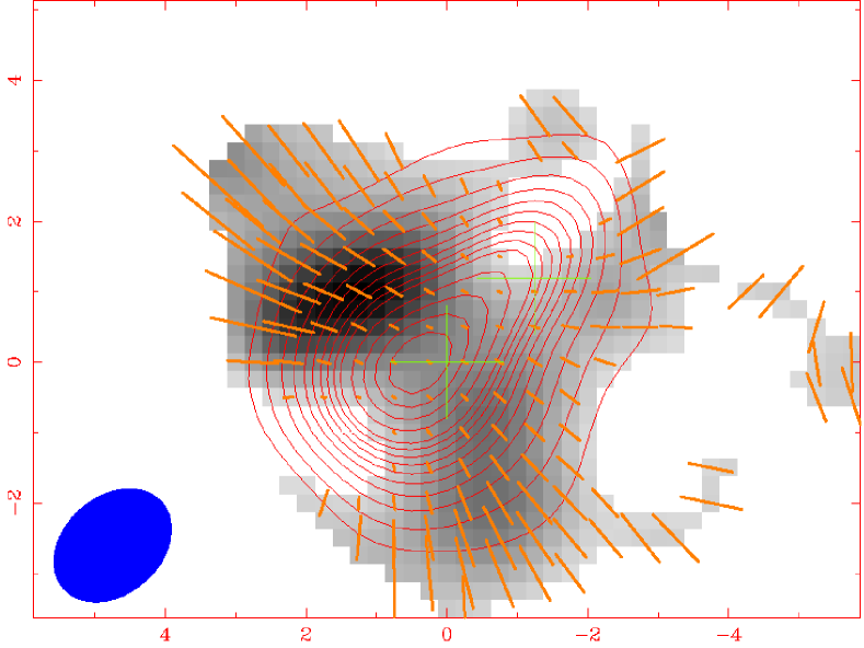
Figure 1: Map of NGC 1333 IRAS 4A, from GRM06. Contours show the continuum emission at 877 $\mu$m, bars indicate the direction and degree of polarization (magnetic field vectors), and the color map shows the polarized intensity. At the distance of 300 pc, $1\arcsec$ corresponds to 300 AU.

2 The models

We have adopted two models for the magnetic field in of IRAS 4A. The first is an axisymmetric, time-dependent, calculation of the inside-out collapse of an uniformly magnetized cloud with ambipolar diffusion (Galli & Shu 1993a,b, hereafter GS93). The second is a steady-state, axisymmetric calculation of the accretion flow on a low-mass protostar and the associated magnetic field, including the effects of Ohmic dissipation (Shu et al. 2006, hereafter S06). Both studies ignore the effects of rotation on the collapse (for this, see Galli et al. 2006).

The study of GS93 focused on the formation of a large flattened structure (“pseudo-disk”) around an accreting protostar due to the effect of the strong non-radial component of the Lorentz force on the collapsing matter. According to GS93, ambipolar diffusion during the dynamical collapse phase plays a minor role on scales larger than a few $10^{2}$ AU, especially at very early times after the onset of collapse. Under quasi-field freezing, the infalling gas pulls the magnetic field towards the center, strongly pinching the field lines near the protostar. The parameters of the GS93 model are the spatial scale of the core prior to collapse, $r_{0}$, and the nondimensional time elapsed since the onset of collapse, $\tau$. The scale $r_{0}$ is defined in terms of the effective sound speed $a_{\rm eff}$ (including thermal, turbulent and magnetic support) and the initial magnetic field $B_{0}$ by the expression $r_{0}=2a_{\rm eff}^{2}/(G^{1/2}B_{0})$, where $G$ is the universal gravity constant. The physical conditions in the core that gave birth to IRAS 4A are difficult to derive. In particular, no Zeeman measurement of the magnetic field strength in the surroundings of IRAS 4A is available. Thus, we adopted the “fiducial” values of GS93, $a_{\rm eff}=0.35$ km s^-1, and $B_{0}=30$ $\mu$G. Then $r_{0}=2.1\times 10^{4}$ AU, and the nondimensional time $\tau$ is given by $\tau=t/t_{0}$ with $t_{0}=r_{0}/a_{\rm eff}=2.9\times 10^{5}$ yr. The results can be easily scaled to different values of $r_{0}$.

The only parameter of the S06 model is the Ohm’s radius, a spatial scale associated with Ohmic dissipation and defined as $r_{\rm Ohm}=\eta^{2}/(2GM_{\star})$, where $\eta$ is the Ohmic resistivity, assumed to be spatially constant. With a non-zero resistivity, the magnetic field lines strongly bent inward by the pull of the infalling gas relax to an almost straight and uniform field configuration in a region of a size $\sim r_{\rm Ohm}$, with the enclosed magnetic flux reduced with respect to the field-freezing value (by a factor of $\sim 100$ at $r=r_{\rm Ohm}$). The value of $\eta$ depends on the ionization, temperature, and chemical composition of the gas close to the source and is not well-constrained. Moreover, the value of $\eta$ is probably associated to macroscopic plasma instabilities rather than microscopic collisional processes (Shu et al. 2007). Estimates of $r_{\rm Ohm}$ are in the range 1–100 AU for a solar-mass star (S06).

3 The method

In spite of the idealization of the models, a comparison with the data is not straightforward. First, the orientation in space of the models is specified by two viewing angles, the position angle $\phi$ of the polar axis with respect to a reference direction in the plane of the sky (with $\phi=0$ corresponding to a polar axis aligned north-south), and the inclination $\psi$ of the meridional plane of the model with respect to the plane of the sky (with $\psi=0$ corresponding to a polar axis in the plane of the sky). These orientation parameters are well-constrained by the observations. In addition, the GS93 model depends on two parameters, a spatial scale $r_{0}$ and time, whereas the steady-state S06 model depends on a single parameter, the Ohm’s radius $r_{\rm Ohm}$. The latter in particular is not well-constrained by the theory (S06). Thus, the data must be compared with an extensive set of model density and magnetic field distributions obtained for different values of the model parameters and the orientation angles $\phi$ and $\psi$.

First from a grid of density and magnetic field models we obtained a large number of maps of Stokes parameters $I$, $Q$, and $U$, using the same method as described in Gonçalves et al. (2005). Once the models were generated, they were convolved with the SMA interferometric response. This was done by converting the modeled map to visibilities using the same distribution of visibilities in the $u,v$ plane and the same $u$, $v$ weighting as the SMA observations of IRAS 4A. This procedure was followed independently for the Stokes $I$, $Q$, and $U$. Once the synthetic SMA–like Stokes $I$, $Q$, $U$ maps were obtained, the polarization intensity and position angle were obtained in the same way for the SMA data and for the models. Since this convolution is nonlinear, it is necessary to scale the model intensity with that of the observations, which is equivalent to selecting a specific value for each map for the product $\kappa B(T)$, or, in other words, a mass calibration factor. This is performed with an iterative procedure.

The third and last step was to compare the modeled and observed polarization angle at each observed position. A quantitive evaluation of the goodness of the fit is given by the standard deviation of the distribution of the residuals between the modeled and the measured polarization angles. The continuum emission and the polarized intensity predicted by the model were also used as additional constraints.

4 Results

4.1 The GS93 model

We have computed a total of 270 maps for $\tau=0.3$, 0.5, and 0.7, with different values of $\phi$ and $\psi$. The best-fit models have $\phi=50^{\circ}$–$60^{\circ}$, $\psi=0^{\circ}$–$30^{\circ}$, $r_{0}=3.2\times 10^{17}$ cm, and $\tau=0.3$. Although the fit is not very sensitive to the value of $\psi$, the best results are obtained for small inclinations of the model with respect to the plane of the sky, with the pseudo-disk seen almost edge-on. In Fig. 2 we show the histograms of the residuals in polarization angles (differences between predicted and observed values) for the three values of $\tau$. The standard deviations are $\sigma=14.8^{\circ}$, $15.6^{\circ}$, and $18.5^{\circ}$ for $\tau=0.3$, $0.5$, and $0.7$ (the instrumental uncertainty on the polarization angles is $\sigma_{\rm instr.}=6.2^{\circ}$, see GRM06).

Although the polarization angles and the intensity profile of IRAS 4A can also be satisfactorily reproduced by models with $\tau=0.5$–0.7, the isocontours of the emitted flux are flatter in these cases than observed, and the polarized flux intensity not reproduced as well as in the $\tau=0.3$ case. For $\tau=0.7$, neither the shape of the isodensity contours nor the polarized intensity distribution can be reasonably reproduced for any possible viewing angle. In Fig. 3 we show a comparison of the modeled and observed intensity and polarization map for the best-fit value $\tau=0.3$. For this case, the largest contribution to $\sigma$ comes from a systematic deviation of the polarization vectors on the top-left side of the map.

With our choice of parameters, the best-fit model with $\tau=0.3$ implies an age for this protostar of $t_{\star}=8.6\times 10^{4}$ yr and a mass of $M_{\star}\approx a_{\rm eff}^{3}t_{\star}/G=0.8$ $M_{\odot}$. The mass of the infalling envelope within a radius $r=10^{3}$ AU from the source is $0.5$ $M_{\odot}$, in agreement with the mass distribution derived by Belloche et al. (2006) from interferometric and single-dish continuum observations ($0.7$ and $0.9$ $M_{\odot}$, respectively). From the best-fit model, the magnetic flux enclosed in a radius $r=10^{3}$ AU is $\Phi=2.4\times 10^{30}$ G cm², so the mass-to-flux ratio of the envelope plus star is $\sim 1.7$ times the critical value $(M/\Phi)_{\rm cr}=(2\pi G^{1/2})^{-1}$, in agreement with the independent estimate of GRM06. Since the effects of ambipolar diffusion are negligible on the collapse time scale in the GS93 model, this value characterizes the mass-to-flux ratio of the original 1.3 $M_{\odot}$ of cloud core that have collapsed to form the protostar and the envelope.

Figure 2: Histogram of residuals in polarization angles for the GS93 models. Solid line, $\tau=0.3$; short-dashed line, $\tau=0.5$ AU; long-dashed line, $\tau=0.7$ (histograms slightly displaced for clarity). The dotted curve shows the Gaussian distribution of the measurement uncertainty with $\sigma_{\rm instr.}=6.2^{\circ}$ (GRM06).

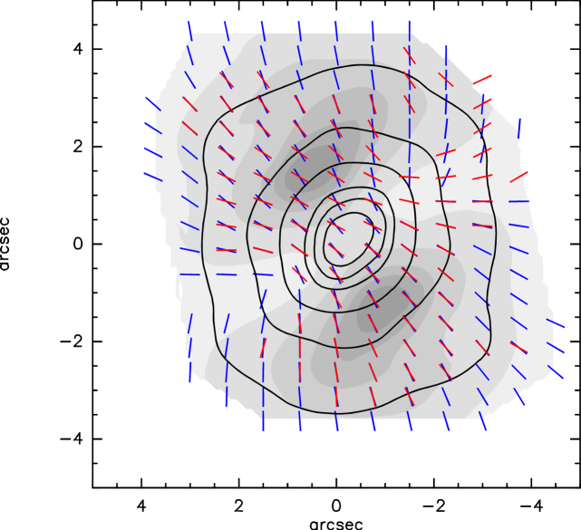
Figure 3: Synthetic maps for the GS93a model: continuum emission (contours), polarized emission (greyscale), polarization degree (segments). Red segments show the observed polarization vectors. Model GS93 with $\tau=0.3$, $\psi=30^{\circ}$, $\phi=55^{\circ}$.

4.2 The S06 model

The S06 model is only applicable to a small region with respect to $a_{\rm eff}t$ ($\approx 6000$ AU with the parameters of Sect. 4.1), and assumes steady-state over this region. Thus, no ages or stellar masses can be derived for this model. In principle, a comparison of the polarization data for IRAS 4A with the S06 model is able to constrain the value of $r_{\rm Ohm}$ without relying on uncertain estimates for the Ohmic resistivity.

For the S06 model, we computed a total of $\sim 450$ synthetic maps with different values of $\phi$ and $\psi$ and values of $r_{\rm Ohm}$ ranging from 5 to 500 AU. Best-fitting models are obtained with $\phi=60^{\circ}$–$65^{\circ}$ and $\psi=25^{\circ}$–$55^{\circ}$. The results for the GS93 model discussed in Sect. 4.1 are not very sensitive to the value of $\psi$, and the observed polarization pattern alone is not sufficient for constraining the model parameters. Models with high values of $r_{\rm Ohm}$ ($r_{\rm Ohm}\approx 200$–500 AU) are not able to reproduce the observed polarization pattern very well or even the two-lobe structure of the polarized continuum emission. The best fit to the polarization angles is obtained for models with $r_{\rm Ohm}\la 50$ AU, suggesting that the actual value of $r_{\rm Ohm}$ may be close to or below the spatial resolution of the observations ($\sim 10^{2}$ AU). In fact, the two-lobe shape of the polarized intensity emission evident in Fig. 1 can only be reproduced with very low values of the Ohm’s radius, $r_{\rm Ohm}=5$–50 AU, suggesting, in agreement with the findings of Sect. 4.1, that the magnetic field down to the scale of resolution is dominated by a pinched, rather than uniform, component. Figure 4 shows the histograms of the polarization angle residuals for the models with $r_{\rm Ohm}=5$, 50 and 500 AU, characterized by standard deviations $\sigma=11.7^{\circ}$, $13.8^{\circ}$, and $22.6^{\circ}$. The polarization and intensity map for the case $r_{\rm Ohm}=5$ AU is shown in Fig. 5.

Figure 4: Histogram of residuals in polarization angles for the S06 models. Solid line, $r_{\rm Ohm}=5$ AU; short-dashed line, $r_{\rm Ohm}=50$ AU; long-dashed line, $r_{\rm Ohm}=500$ AU (histograms slightly displaced for clarity). The dotted curve shows the measurement uncertainty as in Fig. 2.

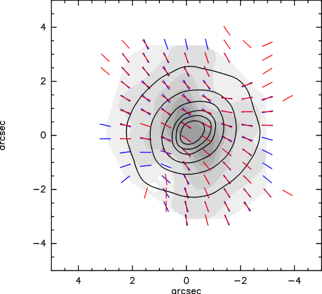
Figure 5: Synthetic maps for the S06 model: continuum emission (contours), polarized intensity (contours and greyscale), polarization degree (segments). Red segments show the observed polarization vectors. Model with $r_{\rm Ohm}=5$ AU, $\psi=54^{\circ}$, $\phi=65^{\circ}$.

5 Discussion and conclusions

From the discussion of Sect. 4, it is clear that the agreement of magnetic collapse models with the continuum polarization data for IRAS 4A is very good, supporting the standard theoretical scenario for the formation of low-mass stars from magnetized molecular cloud cores. The residuals distributions indicate that the best agreement with the data is obtained with GS93 models with early ages ($\sigma=14.8^{\circ}$ for $\tau=0.3$) or for S06 models with low values of the Ohm’s radius ($\sigma=11.7^{\circ}$ for $r_{\rm Ohm}=5$ AU). The low value of $r_{\rm Ohm}$ obtained from the best-fitting S06 model ($r_{\rm Ohm}=5$–50 AU) might also indicate that the steady-state conditions assumed in that model have not yet been reached, and the size of the region of strong magnetic dissipation is below the resolution limit of the observation. At any rate, both models suggest that the magnetic field lines in a region of radius $\sim 500$ AU from the central source(s) are almost radial, as expected for collapse under ideal MHD conditions.

The almost radial geometry of magnetic field lines in IRAS 4A is also supported by the distribution of polarized intensity shown in Fig. 1. In fact, only models with strong central concentration of magnetic field lines reproduce the observed two-lobe structure of the observed polarized intensity, with two large “polarization holes” in the midplane of the pseudo-disk, on both sides of the central protostar. Rather than a variable efficiency alignement of dust grains, the presence and extent of these “holes” seem to indicate a combination of geometrical effect (many field lines point to the observer in a strongly pinched geometry) combined with beam dilution effects (the pinched region is smaller than the beam), resulting in a cancellation of Stokes parameters along the line-of-sight.

Some amount of field dissipation must have already occurred in the central regions of IRAS 4A. The presence of two continuum peaks in IRAS 4A separated by $1.8\arcsec$ (Looney et al 2000; Reipurth et al 2002), corresponding to 540 AU at the assumed distance of 300 pc, suggests that some fragmentation of the pseudo-disk has already occurred, leading to the formation of a (possibly bound) protobinary system. Without field dissipation, the catastrophic magnetic braking associated to the concentration of magnetic fields in ideal-MHD collapse calculation provides a fierce opposition to fragmentation and to the formation of circumstellar disks (Galli et al. 2006; Hennebelle & Fromang 2008; Mellon & Li 2008).

From the distribution of residuals of the fit, it is possible to estimate the relative magnitude of the turbulent vs. the ordered component of the magnetic field using the formula $|\delta{\bf B}|/|{\bf B}|\approx(\sigma^{2}-\sigma_{\rm instr.}^{2})^{1/2}$ (GRM06). With the $\sigma$ obtained for the best-fitting GS93 and S06 models, we derive $|\delta{\bf B}|/|{\bf B}|\approx 20\%$. This is probably an upper limit on the intensity of the turbulent field. Thus, The magnetic field morphology in IRAS 4A is consistent with the standard theoretical scenario for the formation of low-mass stars from cores threaded by ordered rather than turbulent magnetic fields.