Exploring Effective Three-body Forces

Abstract

Topics related to the construction, phenomenological determination, and effects of the effective three-body forces within the traditional nuclear shell model approach are discussed. The manifestations of the three-body forces in realistic nuclei in the $0f_{7/2}$ and $1s0d$ shell model valence spaces are explored.

1 Introduction

In this work we investigate the role that three-body forces play within the nuclear shell model (SM) approach. Establishment of the effective interaction parameters, study of hierarchy in strength from single-particle (s.p.) to two-body, three-body, and beyond, manifestations in energy spectra and transitions rates, comparison with different traditional SM calculations, and overall assessment for the need of beyond-two-body SM are the topics for this discussion. Previous works in this direction have shown an improved description of nuclear spectra Eisenstein:1973 ; Poves:1981 ; Hees:1989 ; Hees:1990 ; Volya:2008 ; Volya:arxiv and the significance of three-body monopole renormalizations Zuker:2003 .

The effective interaction Hamiltonian of rank $k$ is a sum

$$H_{k}=\sum_{n=1}^{k}H^{(n)},\,\,\,{\rm where}\,\,H^{(n)}=\sum_{\alpha\beta}\sum_{L}V_{L}^{(n)}(\alpha\beta)\sum_{M=-L}^{L}\,T_{LM}^{(n)^{\dagger}}(\alpha)\,T_{LM}^{(n)}(\beta),$$ (1)

is the $n$-body rotationally invariant component of the interaction. The $n$-particle creation operators $T_{LM}^{(n)^{\dagger}}(\alpha)$ with the total angular momentum $L$ and magnetic projection $M$ are normalized $\langle 0|T_{L^{\prime}M^{\prime}}^{(n)}(\alpha^{\prime})\,T_{LM}^{(n)^{\dagger}}(\alpha)|0\rangle=\delta_{\alpha\alpha^{\prime}}\delta_{LL^{\prime}}\delta_{MM^{\prime}}$ and expressed through the s.p. creation operators as $T_{LM}^{(n)^{\dagger}}(\alpha)=\sum_{12\dots n}C_{12\dots n}^{LM}(\alpha)\,a_{1}^{\dagger}a_{2}^{\dagger}\dots a_{n}^{\dagger},$ where index $1$ labels a s.p. state. The choice of coefficients $C_{12\dots n}^{LM}(\alpha)$ that defines a full set of orthogonal operators $T_{LM}^{(n)}(\alpha)$ is generally not unique. For numerical work it is most convenient to use a full set of orthogonal eigenstates $|n;LM\alpha\rangle=T_{LM}^{(n)^{\dagger}}(\alpha)|0\rangle$ of some $n$-particle system Volya:2008 . In the $m$-scheme SM we generate states only for a particular value of the total magnetic projection $M$, the remaining states are obtained by the raising and lowering angular momentum operators. It is possible Volya:2008 , to select a single reference two-body Hamiltonian which then can be used to define all many-body operators $T_{LM}^{(n)^{\dagger}}(\alpha)$ for $n>2.$ The traditional SM Hamiltonian is $H_{2}=H^{(1)}+H^{(2)},$ where the two-body operators $T_{LM}^{(2)^{\dagger}}(\alpha)$ are determined with the help of the Clebsch-Gordan coefficients.

2 Manifestation of three-body forces in f_7/2-shell nuclei

As a first example we present here a study of a single-$j$ $0f_{7/2}$ shell, related discussion may be found in Ref. Volya:arxiv . We consider two types of systems $N=28$ isotones starting from ⁴⁸Ca with protons filling the $0f_{7/2}$ shell and the Z=20, ^40-48Ca isotopes with valence neutrons. The states in these systems that are identified by experiments with the $f_{7/2}$ valence space are listed in Tab. 1. The $f_{7/2}$ shell is unique because of symmetries associated with the quasispin and particle-hole conjugation Talmi:1957 ; Ginocchio:1963 ; McCullen:1964 ; Eisenstein:1973 ; Volya:2002PRC . These symmetries are violated if interaction is beyond the two-body.

		$N=28$			$Z=20$
spin	$\nu$	name	Binding	3B$f_{7/2}$	name	Binding	3B$f_{7/2}$
0	0	48Ca	0	0	40Ca	0	0
7/2	1	49Sc	9.626	9.753	41Ca	8.360	8.4870
0	0	50Ti	21.787	21.713	42Ca	19.843	19.837
2	2	1.554	20.233	20.168	1.525	18.319	18.314
4	2	2.675	19.112	19.158	2.752	17.091	17.172
6	2	3.199	18.588	18.657	3.189	16.654	16.647
7/2	1	51V	29.851	29.954	43Ca	27.776	27.908
5/2	3	0.320	29.531	29.590	.373	27.404	27.630
3/2	3	0.929	28.922	28.992	.593	27.183	27.349
11/2	3	1.609	28.241	28.165	1.678	26.099	26.128
9/2	3	1.813	28.037	28.034	2.094	25.682	25.747
15/2	3	2.700	27.151	27.106	2.754	25.022	24.862
0	0	52Cr	40.355	40.292	44Ca	38.908	38.736
2	$2^{*}$	1.434	38.921	38.813	1.157	37.751	37.509
4	$4^{*}$	2.370	37.986	38.002	2.283	36.625	36.570
4	$2^{*}$	2.768	37.587	37.643	3.044	35.864	36.009
2	$4^{*}$	2.965	37.390	37.183	2.657	36.252	35.741
6	2	3.114	37.241	37.353	3.285	35.623	35.606
5	4	3.616	36.739	36.789	-	-	35.180
8	4	4.750	35.605	35.445	(5.088)	(33.821)	33.520
7/2	1	53Mn	46.915	47.009	45Ca	46.323	46.406
5/2	3	0.378	46.537	46.560	.174	46.149	46.280
3/2	3	1.290	45.625	45.695	1.435	44.888	44.991
11/2	3	1.441	45.474	45.454	1.554	44.769	44.763
9/2	3	1.620	45.295	45.309	-	-	44.933
15/2	3	2.693	44.222	44.175	(2.878)	(43.445)	43.214
0	0	54Fe	55.769	55.712	46Ca	56.717	56.728,
2	2	1.408	54.360	54.286	1.346	55.371	55.501
4	2	2.538	53.230	53.307	2.575	54.142	54.332
6	2	2.949	52.819	52.890	2.974	53.743	53.659
7/2	2	55Co	60.833	60.893	47Ca	63.993	64.014
0	0	56Ni	67.998	67.950	48Ca	73.938	73.846

Table 1: States in $f_{7/2}$ valence space with spin and seniority listed in the first and second columns. The $*$ denotes seniority mixed states in 3B$f_{7/2}$. Following are columns with data for $N=28$ isotones and $Z=20$ isotopes. Three columns for each type of valence particles list name and excitation energy, experimental binding energy, and energy from the three-body SM calculation discussed in the text. All data is in units of MeV.

2.1 Particle-hole symmetry

The violation of the particle-hole symmetry is due to monopole terms that are non-liner in the particle-number density. These terms in the Hamiltonian appear from three-body and higher rank interactions Zuker:2003 . For a single-$j$ and a standard two-body SM the symmetry is exact and it makes the spectra of $N$ and $\tilde{N}=\Omega-N$ particle systems identical, apart from a constant shift in energy, here $\Omega=2j+1$. The particle-hole conjugation operator $\mathcal{C}$ that acts on a s.p. state as $\tilde{a}_{jm}^{\dagger}\equiv\mathcal{C}a_{jm}^{\dagger}\mathcal{C}^{-1}=(-1)^{j-m}a_{j-m},$ transforms an arbitrary $n$-body interaction into itself plus some Hamiltonian of a lower interaction-rank $H^{\prime}_{n-1},$ namely $\tilde{H}^{(n)}=(-1)^{n}H^{(n)}+H^{\prime}_{n-1}.$ The $n=1$ case represents a particles to holes transformation $\tilde{N}=-N+\Omega.$ For the $n=2$ it leads to a monopole shift

$$\tilde{H}^{(2)}=H^{(2)}+(\Omega-2N)M,\,\,M=\frac{1}{\Omega}\sum(2L+1)V_{L}^{(2)}.$$ (2)

Within a single-$j$ one-body Hamiltonian is a constant of motion, being always proportional to $N.$ Thus, following Eq. (2), the two-body interaction is identical for particles and holes, apart from some constant-of-motion term. The interaction of rank 3 and higher violate this symmetry making excitation spectra of $N$ and $\tilde{N}=\Omega-N$ particle systems different. The experimental data in Tab. 1 shows the particle-hole symmetry violations, for example the excitation energies of $\nu=2$ states in $N=2$ system are systematically higher then those in the 6-particle case, indicating a reduced ground state binding. Using this information a monopole component of the three-body force can be extracted from the differences in excitation energies between particle and hole systems, see Fig. 1 and discussion below.

2.2 Seniority

The $j=7/2$ is the largest single-$j$ shell for which the number of unpaired nucleons $\nu$, the seniority, is an integral of motion for any one- and two-body interaction Schwartz:1954 ; Talmi:1957 . Formally, the pair operators $T_{00}^{(2)}$, $T_{00}^{(2)\dagger},$ and particle number $N$ form an SU(2) rotational group, which because of its analogy to angular momentum is referred to as quasispin. The relation is established by the operators

$${\mathcal{L}}_{z}=\frac{N}{2}-\frac{\Omega}{4}\,,\quad\mathcal{L}=\frac{\Omega}{4}-\frac{\nu}{2}$$

with $\mathcal{L}(\mathcal{L}+1)$ being an eigenvalue of the quasispin vector squared and $\mathcal{L}_{z}$ its magnetic projection.

For a spectrum, the invariance under seniority sets relations between states of the same $\mathcal{L}$ but different projection $\mathcal{L}_{z}$. For example, the excitation energies of $\nu=2$ states from the $\nu=0,$ $0^{+}$ ground state are identical in all even-particle systems. Using Wigner-Eckart theorem a full set of relations can be established, see for example sec IIIB in ref. Volya:2002PRC or Ref. Talmi:1993 . The invariance under quasispin rotations allows to classify operators in close analogy to the usual rotations. The s.p. operators associated with the particle transfer reactions carry $\mathcal{L}=1/2$ and thus permit seniority change $\Delta\nu=1$. The reactions ⁵¹V(³He, d)⁵²Cr and ⁴³Ca(d,p)⁴⁴Ca indicate seniority mixing as $\nu=4$ final states are populatedAuerbach:1967 ; Bjerregaard:1967 . The one-body multipole operators are quasispin scalars for odd angular momentum, and quasispin vectors for even. Thus, the $M1$ electromagnetic transitions are given by the quasiscalar operators that do not change quasispin. The $E2$ operator is a quasivector. In the mid-shell for ⁵²Cr and ⁴⁴Ca, where $N=\Omega/2$ and $\mathcal{L}_{z}=0$ the $E2$ transitions between states of the same seniority are forbidden. Seniority can be used to classify the many-body operators $T_{LM}^{(n)}$ and interaction parameters. The three-body interactions mix seniorities, one exception is the interaction between $\nu=1$ nucleon triplets given by the strength $V_{7/2}^{(3)}.$

2.3 Parameter fit and evidence for three-body forces

To obtain the parameters of the effective Hamiltonian with the three-body forces we conduct a full least-square $p=$11 parameter fit to $d=$31 data-point (27 in the case of Ca isotopes). The procedure is similar to a two-body fit outlined for this model space in sec. 3.2 of Ref. Lawson:1980 . Schematically ${\bf E=AV}$ where ${\bf E}$ is a set of 31 energies, ${\bf V}$ is a list of 11 interaction parameters and ${\bf A}$ is 31 by 11 matrix created from the linear form of the Hamiltonian operator Eq. (1). Due to the seniority mixing ${\bf A}$ depends on the eigenstates, which in turn are determined by the interactions ${\bf V};$ thus the overall fitting procedure is iterative Brown:2006 . In this example seniority mixing occurs only in 4 states of the $N=4$ system, in consequence most of the matrix elements of ${\bf A}$ are constants. Using the set of experimental data in Tab. 1, denoted here as ${\bf E}_{ex},$ we determine ${\bf V}=({\bf A}^{T}{\bf A})^{-1}{\bf A}^{T}{\bf E}_{ex}$, where $T$ and $-1$ superscripts indicate transposed and inverted matrices. The obtained interaction parameters are used to update non-constant elements of ${\bf A}.$ The procedure is iterated several times so that the interaction-dependent components of ${\bf A}$ converge. In Tab. 2 the resulting parameters are listed for the $N=28$ proton system, and for the neutron $Z=20$ system. The two columns in each case correspond to fits without (left) and with (right) the three-body forces. The root-mean-square deviation (RMS) $|{\bf E}_{ex}-{\bf AV}|/\sqrt{d}$ is given for each fit. The confidence limits given in brackets are inferred from the variances for each fit parameter

$$\sigma^{2}(V_{j})=\frac{|{\bf E}_{ex}-{\bf AV}|^{2}}{d-p}({\bf A}^{T}{\bf A})_{jj}^{-1}.$$

	$N$=28		$Z$=20
	2B$f_{7/2}$	3B$f_{7/2}$	2B$f_{7/2}$	3B$f_{7/2}$
$\epsilon$	-9827(16)	-9753(30)	-8542(35)	-8486.98(72)
$V_{0}^{(2)}$	-2033(60)	-2207(97)	-2727(122)	-2863(229)
$V_{2}^{(2)}$	-587(39)	-661(72)	-1347(87)	-1340(176)
$V_{4}^{(2)}$	443(25)	348(50)	-164(49)	-198(130)
$V_{6}^{(2)}$	887(20)	849(38)	411(43)	327(98)
$V_{7/2}^{(3)}$		55(28)		53(70)
$V_{5/2}^{(3)}$		-18(70)		2(185)
$V_{3/2}^{(3)}$		-128(88)		-559(273)
$V_{11/2}^{(3)}$		102(43)		51(130)
$V_{9/2}^{(3)}$		122(41)		272(98)
$V_{15/2}^{(3)}$		-53(29)		-24(73)
RMS	120	80	220	170

Table 2: Interaction parameters of 2B$f_{7/2}$ and 3B$f_{7/2}$ SM Hamiltonians determined with the least-square fit are given in keV.

The reduction of the RMS deviation, for example for $Z=28$ isotones it drops from 120 keV to about 80 keV, is not the only evidence in support of the three-body forces. The fit parameters are stable within quoted error-bars even if some questionable data-points are removed. The energies from the three-body fit listed in Tab. 1. are comparable or even better than the results from many two-body SM calculations in the expanded model space Lips:1970 ; Poves:2001 . However, such comparisons are difficult since different models have different number of parameters and were fit to different sets of nuclei.

In Tab. 3 we discuss the renormalization of pairing by considering a minimal fit limited to the ground states and a single three-body term. The fit is similar to Ref. Talmi:1957 , but has a seniority conserving three-body force given by the $\nu=1$ triplet operator $T_{jm}^{(3)}\sim a_{jm}^{\dagger}T_{00}^{(2)}$ with the strength $V_{7/2}^{(3)}$. This interaction is equivalent to a density-dependent pairing force Zelevinsky:2006 . In a single-$j$ shell the renormalization of pairing by a particle-number dependent strength

$$V_{0}^{(2)^{\prime}}=V_{0}^{(2)}+\Omega\frac{N-2}{\Omega-2}V_{j}^{(3)}$$ (3)

allows for an exact treatment of the three-body term. The ground state energies with $\nu=0$ or 1 are

$$E=\epsilon N+\frac{N-\nu}{\Omega-2}\left((\Omega-N-\nu)\frac{V_{0}^{(2)^{\prime}}}{2}+(N-2+\nu)M^{\prime}\right),$$ (4)

which is a usual expression Talmi:1957 ; Volya:2002PRC , but includes a renormalized pairing strength denoted with prime. The results from the minimal fit are shown in Tab. 3, they are consistent with the full fit in Tab. 2.

	$N=28$		$Z=20$
$\epsilon$	-9703(40)	-9692(40)	-8423(51)	-8403(55)
$V_{0}^{(2)}$	-2354(80)	-2409(110)	-3006(120)	-3105(156)
$M$	1196(40)	1166(50)	-823(55)	-876(76)
$V_{7/2}^{(3)}$	-	18(20)	-	31(31)
RMS	50	46	73	65

Table 3: Interaction parameters for the minimal $f_{7/2}$ SM determined with the linear least-squared fit of 8 binding energies. In brackets the variances for each parameter are shown. The two columns for isotopes and isotones are fits without and with the three-body term.

In Fig. 1 we give a cumulative picture showing the $V_{7/2}^{(3)}$ term found with different methods. As discussed above, due to the particle-hole symmetry and seniority conservation, excitation energies of $\nu=2$: $2^{+},\>4^{+},$ and $6^{+}$ states in $N=2,4,$ and 6 -particle systems should be identical. The $V_{7/2}^{(3)}$ coefficient can be found assuming that it is responsible for most of the mass difference. For example, the difference in excitation energies of these states between ⁵⁰Ti and ⁵²Cr equals to $8V_{7/2}^{(3)}/3$. The independent result on $V_{7/2}^{(3)}$ inferred from these observations, the binding energy fit, and the fit to all states in the $N=28$ isotones with 4 parameters are summarized in Fig. 1. The point that corresponds to the $4^{+}$ state in ⁵²Cr in Fig. 1 is not in agreement with the rest of the data, it demonstrates the seniority mixing discussed below.

Figure 1: Cumulative data on $V_{7/2}^{(3)}$ seniority $\nu=1$ effective three-body force in $N=48$ isotones, left, and $Z=40$ isotopes to the right. The point labeled as BE comes from a fit to 8 binding energies in Tab.3 and includes a fitting error-bars. The point labeled as “Full Fit” corresponds to a fit of all 31 levels in $N=28$ isotones with 6 parameters for s.p. energy, two-body force and $V_{7/2}^{(3)}$. Other individual points correspond to extraction of $V_{7/2}^{(3)}$ from excitation energy, always compared to $N=2$ system (⁵⁰Ti or ⁴²Ca)

It follows from Tabs. 2 and 3, and Fig. 1 that within the error-bars the three-body interaction is isospin invariant; it is the same for proton and neutron valence spaces.

2.4 Seniority mixing in ⁵²Cr

The mid-shell case of ⁵²Cr, see Fig.2, is interesting to discuss. Here, in addition to 2B$f_{7/2}$ and 3B$f_{7/2}$ interactions from Tab. 2 we perform a large scale SM calculation 2B$f_{7/2}p$ (includes $p_{1/2}$ and $p_{3/2}$) and 2B$fp$ (entire $fp$-shell, truncated to $10^{7}$ projected m-scheme states) using FPBP two-body SM Hamiltonian Brown:2001 . Similar results in a more restrictive valence space can be found in Ref. Lips:1970 .

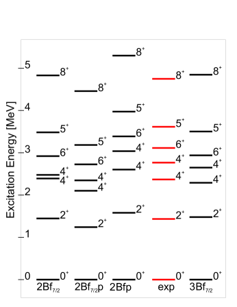
Figure 2: Spectrum of $52$Cr.

The level repulsion between neighboring $4_{1}^{+}$ and $4_{2}^{+}$ states is generated by the seniority mixing, the observed energy difference of 400 keV is not reproduced by the 2B$f_{7/2}$ (84 keV) model. As seen in Fig. 2 the discrepancy remains in the extended two-body model 2B$f_{7/2}p$ (200 keV). Although, the full 2B$fp$ model reproduces the splitting, the excessive intruder admixtures over-bind the ground state and effectively push all states up in excitation energy. The 3B$f_{7/2}$ model is in good agreement with experiment; its predictions for the seniority mixing are $\nu(4_{1}^{+})=2.82$ and $\nu(4_{2}^{+})=2.71,$ as calculated from the expectation value of the pair operator $\langle T_{00}^{(2)^{\dagger}}T_{00}^{(2)}\rangle=(N-\nu)(2j+3-N-\nu)/(4j+2).$ The $2_{1}^{+}$ state is relatively pure $\nu(2_{1}^{+})=2.006$.

The seniority mixing violates quasispin selection rules Armstrong:1965 ; Bjerregaard:1967 ; McCullen:1964 ; Monahan:1968 ; Pellegrini:1973 which in the past have been explained by the two-body models beyond the single-$j$ Auerbach:1967 ; Engeland:1966 ; Ginocchio:1963 ; Lips:1970 ; McCullen:1964 , however such models not always describe all of the features observed in experiment. In particular, to explain electromagnetic transitions sizable variations of effective charges are needed Brown:1974 and the particle transfer spectroscopic factors do not show large amount of strength outside the $f_{7/2}$ valence space Armstrong:1965 . In Tab. 4 $B(E2)$ transitions rates from all models are compared to experiment. To make a fair comparison the combination of the nuclear radial overlap and effective charge is normalized using observed $E2$ rate for the transition $2_{1}\rightarrow 0_{1}$ in the 2B$f_{7/2}$, 2B$f_{7/2}p,$ and 2B$fp$ models. The parameter for the 3B$f_{7/2}$ model is identical to the one used in the 2B$f_{7/2}.$ The small difference in $2_{1}\rightarrow 0_{1}$ $B(E2)$ between the 3B$f_{7/2}$ and 2B$f_{7/2}$ models is a result of the $\nu=4$ admixture in the $2_{1}^{+}$ state. The strong $\nu=4$ and $\nu=2$ seniority mixing between $4_{1}^{+}$ and $4_{2}^{+}$ states impacts forbidden transitions; for example, $E2$ transitions $4_{2}\rightarrow 2_{1}$ and $6_{1}\rightarrow 4_{2}$ become allowed.

	2B$f_{7/2}$	2B$f_{7/2}p$	2B$fp$	3B$f_{7/2}$	Experiment
$2_{1}\rightarrow 0_{1}$(∗)	118.0	118.0	118	117.5	118$\pm 35$
$4_{1}\rightarrow 2_{1}$	130.4	122.5	105.8	73.2	83$\pm 15$(1,2)
$4_{2}\rightarrow 2_{1}$	0	3.3	15.1	56.8	69$\pm 18$
$4_{2}\rightarrow 4_{1}$	125.2	59.3	2.6	0.5
$2_{2}\rightarrow 0_{1}$	0	0.003	0.9	0.5	0.06$\pm 0.05$
$2_{2}\rightarrow 2_{1}$	119.2	102.2	101.9	117.1	150$\pm 35$
$2_{2}\rightarrow 4_{1}$	0	10.8	34.4	19.9
$2_{2}\rightarrow 4_{2}$	57.8	7.2	5.2	38.7
$6_{1}\rightarrow 4_{1}$	108.9	86.2	56.3	57.8	59$\pm 20^{(1)}$
$6_{1}\rightarrow 4_{2}$	0	9.3	27.6	51.1	30$\pm 10^{(1)}$

Table 4: B(E2) transition summary on ⁵²Cr expressed in units $e^{2}$fm⁴. The data is taken from Huo:2007 . ^(∗)In the 2B $f_{7/2}p$ and 2B$fp$ models we use $0.5$(neutron) and $1.5$(proton) effective charges, the overall radial scaling is fixed by the B(E2,$2_{1}\rightarrow 0_{1}$). ⁽¹⁾The life-time error-bars were used. ⁽²⁾There are conflicting results on life-time; we use DSAM (HI, x$n\gamma$) data from Ref. Huo:2007 , which is consistent with Brown:1974 .

The proton removal spectroscopic factors in Tab. 5 show a similar picture, where the seniority mixing has a strong impact on transitions. In support of the three-body forces as a source of the mixing it was argued in Ref. Armstrong:1965 that the sum of spectroscopic factors for $4^{+}$ states is close to 4/3 which is consistent with the observation in Ref. Armstrong:1965 and does not support the expanded valence space where spectroscopic factors are reduced due to fragmentation of the single-particle strength.

	2B$f_{7/2}$	2B$f_{7/2}p$	2B$fp$	3B$f_{7/2}$	Exp
$0{}_{1}^{+}$	4.00	3.73	3.40	4.00	4.00
$2{}_{1}^{+}$	1.33	1.14	0.94	1.33	1.08
$4{}_{1}^{+}$	0.00	0.13	0.34	0.63	0.51
$4{}_{2}^{+}$	1.33	1.11	0.70	0.71	0.81
$6{}_{1}^{+}$	1.33	1.28	1.28	1.33	1.31

Table 5: Proton removal spectroscopic factors. The experimental data is taken from ⁵¹V(³He,d)⁵²Cr reaction Armstrong:1965 . Within error-bars this data is consistent with results Huo:2007 .

3 Three-body forces in oxygen isotopes

The above single-$j$ example is remarkable due to its transparency and simplicity. The general SM case, however, is complicated by an enormously large number of parameters and thus difficulty of the fit Poves:1981 ; Hees:1989 ; Hees:1990 ; Zuker:2003 . Selecting dynamically relevant components of the many-body forces requires an in-depth microscopic understanding of their origin. Establishment of the physically relevant set of the operator basis $T_{LM}^{(n)^{\dagger}}(\alpha)$ is an important start. As discussed in the introduction, for $n>2$ the index $\alpha$ must include an additional information about the coupling scheme, the choice of which is not unique. Previous ideas on selecting the best set of triplet operators include a possibility of using the $\nu=1$ operators for each single-particle level Zelevinsky:2006 . For $j=7/2$ the three-body force associated with this operator, discussed in Fig. 1, is indeed a dominating component in binding. However, it is not clear if such construction, built upon s.p. levels, is the best choice in a general case given renormalization of the s.p. effective degrees of freedom by the two-body interaction. The two-body Hamiltonian of the pairing type would, for instance, suggest the use of quasiparticles.

Perusing this idea we propose an alternative approach which assumes a hierarchy of forces, where higher rank components of the Hamiltonian are perturbative, and the operator basis are selected using the many-body dynamics.

Consider $H_{n-1}$, $n\geq 3$ Hamiltonian to be determined by some procedure. While building a higher rank forces $H_{n}=H_{n-1}+H^{(n)}$, we assume $H^{(n)}$ to be perturbatively small. Thus, within the lowest order perturbation theory the $n$-particle wave-functions of $H_{n-1}$ and $H_{n}$ are the same and can be found by diagonalizing $H_{n-1}$

$$H_{n-1}|n;LM\alpha\rangle=E_{n;L}(\alpha)\,|n;LM\alpha\rangle.$$

We use these eigenstates to define a full set of $n$-body operators $T_{LM}^{(n)}(\alpha)$ as $|n;LM\alpha\rangle=T_{LM}^{(n)^{\dagger}}(\alpha)|0\rangle,$ which we view as the most relevant basis. With a perturbative nature in mind the term $H^{(n)}$ is diagonal in these basis, $V_{L}^{(n)}(\alpha\beta)=0$ if $\alpha\neq\beta.$ Thus, the number of parameters is reduced. Further steps can be taken to discuss the significance of the diagonal parameters. When pairing is important one can take only those states (basis operators) that correspond to the lowest quasiparticle excitations. Experimental data can be used for guidance. For example, if the $n$-particle states are known and identified experimentally to have energies $E_{L}^{(exp)}(n;\alpha),$ a direct fit can be done by setting the corresponding $n$-body interaction parameters as $V_{L}^{(n)}(\alpha,\alpha)=E_{n;L}^{(exp)}(\alpha)-E_{n;L}(\alpha),$ so that the new Hamiltonian reproduces exactly the experimental energies.

There are some issues to stress. Certainly, the transition from $n=1$ to $n=2$, is not a subject to this approach. One has to have a starting SM Hamiltonian $H_{SM}^{(2)}$ determined from G-matrix techniques or by other methods, see Brown:2001 and references therein. It is possible to rewrite the two-body Hamiltonian as a diagonal structure by introducing new pair operators, this is useful for perturbative adjustments of the two-body interactions.

The two-body SM Hamiltonian can be used as a primary component of interaction, defining many-body operators, and treating all higher rank forces as perturbations. It is important for this approach to stay within the perturbation theory. Departing a perturbative form, it is feasible with this construction to create a Hamiltonian that exactly reproduces energies of all states within a given valence space, tests show that in this case the many-body forces have an inverse hierarchy with higher rank ones giving a bigger contribution.

It is an established practice in the SM approach to include a mass dependence of the two-body forces. For a short range delta-type interaction the radial overlap integrals scale as $R^{-3/2}$, where $R$ is the radius of the nucleus. Thus, in terms of the mass-number $A$ the two-body interaction $H^{(2)}\sim A^{-1/2}.$ At the opposite extreme the long-range Coulomb leads to an $A^{-1/6}$ scaling. The fits to experimental data lead to a compromising middle value $A^{-0.3}$Brown:2006 . The many-body forces are expected to be short range, requiring all participating particles to be localized. The resulting scaling that follows from this argument is

$$H^{(n)}\sim A^{(1-n)/2}\,,{\rm so}\quad H^{(n)}(A)=\left(\frac{A_{c}+n}{A}\right)^{(n-1)/2}H^{(n)}(A_{c}),$$ (5)

where $A_{c}$ is the mass of the core. At this stage it is not clear if this argument is valid and if scaling should be included.

As a demonstration we discuss here a 3-body force in the case of oxygen isotopes. For the two-body interaction Hamiltonian we take a USD shell model USD . The total number of triplet operators, not counting magnetic projections, is 37 which in a general 3-body interaction Hamiltonian gives a large number of parameters. Examination of experimental data for ¹⁹O and results from the different shell model Hamiltonians USD, USDA and USDB Brown:2006 show a rather systematic difference; in particular for the lowest $5/2^{+}_{1}$, $3/2^{+}_{1}$ and $1/2^{+}_{1}$ states. These are one quasiparticle excitations. Thereby, we define the corresponding triplet operators $T_{jm}^{(3)^{\dagger}}$ with $j=5/2,\,3/2,$ and 1/2 from the three-particle eigenstates of the USD Hamiltonian; and specify the three-body interaction in the diagonal form

$$H^{(3)}=\sum_{j=5/2,3/2,1/2}\,V_{j}^{(3)}\sum_{m=-j}^{j}\,T_{jm}^{(n)^{\dagger}}\,T_{jm}^{(n)}.$$ (6)

For Fig. 3 we fit the three parameters in Eq. (6) to the ground states in even systems and to the three lowest states with one unpaired particle in the odd systems for mass $A=19$ to 22 oxygen isotopes. The values from the best fit are $V^{(3)}_{5/2}=45$ keV, $V^{(3)}_{3/2}=-179$ keV, and $V^{(3)}_{3/2}=-231$ keV.

The improvement in the spectrum, seen in Fig. 3 is significant. Certainly, this first study is to be continued, there is a possibility to examine more interaction terms, discuss scaling of the matrix elements, and to consider fitting all parameters for one-, two-, and three-body components together. Modifying perturbatively the two-body part should not invalidate the quality of the USD-defined three-body basis.

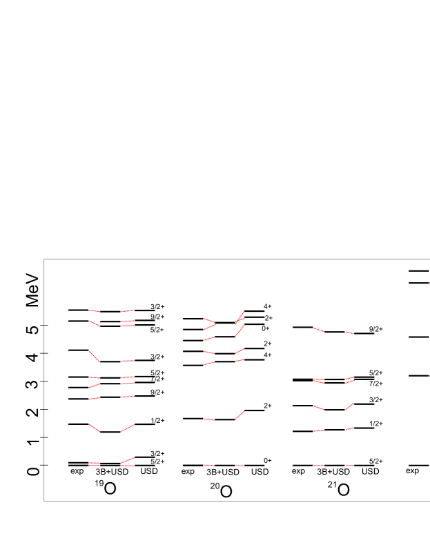
Figure 3: Spectrum of ^19-22O isotopes. For every nucleus, experimentally observed states are compared with the spectrum that includes three-body forces and with the two-body USD SM Hamiltonian, from left to right, as identified at the bottom.

4 Conclusion

Dealing with many-body forces, understanding their origins, structure, and hierarchy of renormalizations is an important component for a successful solution of a many-body problem. This presentations aims to continue the discussion in Ref. Eisenstein:1973 ; Poves:1981 ; Hees:1989 ; Hees:1990 ; Zuker:2003 ; Volya:2008 ; Volya:arxiv related to the phenomenological three-body forces within the context of the nuclear shell model approach. The study of nuclei in the $0f_{7/2}$ shell shows evidence of such forces through an overall fit to data with full examination of uncertainties, via examination of binding energies and associated differences in excitation spectra, and with an in-depth analysis of violations of symmetries in the structure of wave functions.

The general SM problem with many-body forces is complicated by a large number of parameters, the absence of a good microscopic approach, difficulties in fits and questions related to renormalizations of strengths. These issues are discussed and some methods for dealing with them are proposed. In particular, in analogy to a Hartree-Fock procedure where single-particle states are defined in the way to best represent the dynamics of the system, we propose here methods to identify the most relevant many-body operators. These techniques are demonstrated using a chain of oxygen isotopes.

Support from the U. S. Department of Energy, grant DE-FG02-92ER40750 is acknowledged.

References

- (1) I. Eisenstein and M. W. Kirson, Phys. Lett. B, 47, 315 (1973).
- (2) A. Poves and A. Zuker, Phys. Rep. 70, 235 (1981).
- (3) A. van Hees, J. Booten, and P. Glaudemans, Phys.Rev.Lett. 62, 2245 (1989).
- (4) A. van Hees, J. Booten, and P. Glaudemans, Nucl. Phys. A, 507, 55 (1990).
- (5) A. Volya, Phys. Rev. Lett. 100, 162501 (2008).
- (6) A. Volya, (2008), arXiv:0805.0291, accepted for publication in Phys. Rev. C.
- (7) A. P. Zuker, Phys.Rev.Lett. 90, 042502 (2003).
- (8) I. Talmi, Phys.Rev. 107, 326 (1957).
- (9) J. N. Ginocchio and J. B. French, Phys. Lett. 7, 137 (1963).
- (10) J. D. McCullen, B. F. Bayman, and L. Zamick, Phys.Rev. 134, B515 (1964).
- (11) A. Volya, Phys. Rev. C 65, 044311 (2002).
- (12) C. Schwartz and A. deShalit, Phys.Rev. 94, 1257 (1954).
- (13) I. Talmi, Simple Models of Complex Nuclei: The Shell Model and Interacting Boson Model (Harwood Academic Pub, 1993).
- (14) N. Auerbach, Phys. Lett. B, 24, 260 (1967).
- (15) J. H. Bjerregaard and O. Hansen, Phys.Rev. 155, 1229 (1967).
- (16) R. D. Lawson, Theory of the nuclear shell model (Clarendon Press, 1980).
- (17) B. A. Brown and W. A. Richter, Phys. Rev. C 74, 034315 (2006).
- (18) K. Lips and M. T. McEllistrem, Phys.Rev.C 1, 1009 (1970).
- (19) A. Poves, J. Sanchez-Solano, E. Caurier, and F. Nowacki, Nucl. Phys. A 694, 157 (2001).
- (20) V. Zelevinsky, T. Sumaryada, and A. Volya, 2006, BAPS.2006.APR.C8.4.
- (21) B. A. Brown, Prog. Part. Nucl. Phys. 47, 517 (2001).
- (22) D. D. Armstrong and A. G. Blair, Phys.Rev. 140, B1226 (1965).
- (23) C. F. Monahan, et.al., Nucl. Phys. A, 120, 460 (1968).
- (24) F. Pellegrini, I. Filosofo, M. I. E. Zaiki, and I. Gabrielli, Phys.Rev.C 8, 1547 (1973).
- (25) T. Engeland and E. Osnes, Phys. Lett. 20, 424 (1966).
- (26) B. A. Brown, et.al., Phys.Rev.C 9, 1033 (1974).
- (27) J. Huo, S. Huo, and C. Ma, Nuclear Data Sheets, 108, 773 (2007).
- (28) E. K. Warburton and B. A. Brown, Phys. Rev. C 46, 923 (1992).