Root polytopes and growth series of root lattices

Abstract.

The convex hull of the roots of a classical root lattice is called a root polytope. We determine explicit unimodular triangulations of the boundaries of the root polytopes associated to the root lattices $A_{n}$, $C_{n}$ and $D_{n}$, and compute their $f$-and $h$-vectors. This leads us to recover formulae for the growth series of these root lattices, which were first conjectured by Conway–Mallows–Sloane and Baake–Grimm and proved by Conway–Sloane and Bacher–de la Harpe–Venkov.

1. Introduction

A lattice ${\mathcal{L}}$ is a discrete subgroup of ${\mathbb{R}}^{n}$ for some $n\in{\mathbb{Z}}_{>0}$. The rank of a lattice is the dimension of the subspace spanned by the lattice. We say that a lattice ${\mathcal{L}}$ is generated as a monoid by a finite collection of vectors ${\mathcal{M}}=\{{\mathbf{a}}_{1},\dots,{\mathbf{a}}_{r}\}$ if each ${\mathbf{u}}\in{\mathcal{L}}$ is a nonnegative integer combination of the vectors in ${\mathcal{M}}$. For convenience, we often write the vectors from ${\mathcal{M}}$ as columns of a matrix $M\in{\mathbb{R}}^{n\times r}$, and to make the connection between ${\mathcal{L}}$ and $M$ more transparent, we refer to the lattice generated by $M$ as ${\mathcal{L}}_{M}$. The word length of ${\mathbf{u}}$ with respect to ${\mathcal{M}}$, denoted $\operatorname{w}({\mathbf{u}})$, is $\min(\sum c_{i})$ taken over all expressions ${\mathbf{u}}=\sum c_{i}{\mathbf{a}}_{i}$ with $c_{i}\in{\mathbb{Z}}_{\geq 0}$. The growth function $\operatorname{S}(k)$ counts the number of elements ${\mathbf{u}}\in{\mathcal{L}}$ with word length $\operatorname{w}({\mathbf{u}})=k$ with respect to ${\mathcal{M}}$. We define the growth series to be the generating function $G(x):=\sum_{k\geq 0}\operatorname{S}(k)\,x^{k}$. It is a rational function $G(x)=\frac{h(x)}{(1-x)^{d}}$ where $h(x)$ is a polynomial of degree less than or equal to the rank $d$ of ${\mathcal{L}}_{M}$ [4]. We call $h(x)$ the coordinator polynomial of the growth series. It is important to keep in mind that these functions all depend on the choice of generators for the monoid.

In this paper we examine the growth series for the classical root lattices $A_{n}$, $C_{n}$ and $D_{n}$, generated as monoids by their standard set of generators. Conway and Sloane [7] proved an explicit formula for the growth series for $A_{n}$ and, with Mallows’s help, conjectured one for the $D_{n}$ case. Baake and Grimm [1] later conjectured formulae for the $B_{n}$ and $C_{n}$ cases. Bacher, de la Harpe, and Venkov [2] subsequently provided the proofs of all these cases. We give alternative proofs of the formulae in the cases $A_{n},C_{n},$ and $D_{n}$, by computing the $f$-vector of a unimodular triangulation of the corresponding root polytope.

The approach presented here is a natural extension of the proofs related to the growth series of cyclotomic lattices given in [3]. We let ${\mathcal{P}}_{{\mathcal{M}}}$ be the polytope formed by the convex hull of the generating vectors in ${\mathcal{M}}$. For the lattices we consider, this polytope is the root polytope of the corresponding lattice. We determine explicit unimodular triangulations of these polytopes and show that the $h$-polynomial of these triangulations (hence, of any unimodular triangulation) is identical to the coordinator polynomial $h(x)$ for the respective root lattice. Our method implies that $h(x)$ is necessarily palindromic and must have nonnegative coefficients; this is confirmed by the formulae. Incidentally, since the coordinator polynomial for the growth series of the root lattice $B_{n}$ is not palindromic, our approach would need to be modified to prove the formula in the $B_{n}$ case.

To state our main results, let $A_{n}$, $C_{n}$, and $D_{n}$ be the classical root lattices generated as monoids by

$${\mathcal{M}}_{A_{n}} = \{{\mathbf{e}}_{i}-{\mathbf{e}}_{j}:0\leq i,j\leq n+1\}$$

$${\mathcal{M}}_{C_{n}} = \{\pm 2{\mathbf{e}}_{i}:1\leq i\leq n\,;\,\pm{\mathbf{e}}_{i}\pm{\mathbf{e}}_{j}:1\leq i\neq j\leq n\},$$

$${\mathcal{M}}_{D_{n}} = \{\pm{\mathbf{e}}_{i}\pm{\mathbf{e}}_{j}:1\leq i\neq j\leq n\},$$

respectively, and define the classical root polytopes ${\mathcal{P}}_{A_{n}}=\operatorname{conv}{\mathcal{M}}_{A_{n}}$, ${\mathcal{P}}_{C_{n}}=\operatorname{conv}{\mathcal{M}}_{C_{n}}$, and ${\mathcal{P}}_{D_{n}}=\operatorname{conv}{\mathcal{M}}_{D_{n}}$ to be the convex hulls of these generating sets.

The $f$-vector of a simplicial complex $\Gamma$ is given by $f(\Gamma)=(f_{-1},f_{0},f_{1},\dots,f_{n-1})$ where $f_{i}$ is the number of $i$-dimensional faces of $\Gamma$; by convention $f_{-1}=1$. The $f$ and $h$-polynomials of $\Gamma$ are defined [17] to be

$$f_{\Gamma}(x)=\sum_{i=-1}^{d}f_{i}\,x^{d-i}\qquad h_{\Gamma}(x)=f_{\Gamma}(x-1)=\sum_{i=-1}^{d}f_{i}\,(x-1)^{d-i}.$$

Theorem 1.

Let $f_{A_{n}}(x)$, $f_{C_{n}}(x)$, and $f_{D_{n}}(x)$ be the $f$-polynomials of any unimodular triangulations of the boundaries of the classical root polytopes. Then

$$f_{A_{n}}(x) = \sum_{m=0}^{n}{n+m\choose m,m,n-m}x^{n-m},$$

$$f_{C_{n}}(x) = \sum_{m=0}^{n}\frac{n\,2^{2m}}{n+m}\binom{n+m}{2m}x^{n-m},$$

$$f_{D_{n}}(x) = \sum_{k=0}^{n}\left(\frac{n\,2^{2m}}{n+m}\binom{n+m}{2m}-\frac{n(2n-m-1)2^{m-1}}{n-m}{n-2\choose m-1}\right)x^{n-m}.$$

Theorem 2.

[2, 7] The coordinator polynomial of the growth series of the classical root lattices $A_{n},C_{n},$ and $D_{n}$ with respect to the generating sets ${\mathcal{M}}_{A_{n}},{\mathcal{M}}_{C_{n}}$, and ${\mathcal{M}}_{D_{n}}$ is equal to the $h$-polynomial of any unimodular triangulation of the respective polytopes ${\mathcal{P}}_{A_{n}}$, ${\mathcal{P}}_{C_{n}}$, and ${\mathcal{P}}_{D_{n}}$. These polynomials are palindromic and have nonnegative coefficients. More specifically,

$$h_{A_{n}}(x)=\sum_{k=0}^{n}\binom{n}{k}^{2}x^{k},\quad h_{C_{n}}(x)=\sum_{k=0}^{n}\binom{2n}{2k}x^{k},\quad h_{D_{n}}(x)=\sum_{k=0}^{n}\left[\binom{2n}{2k}-\frac{2k(n-k)}{n-1}\binom{n}{k}\right]x^{k}.$$

2. Finding growth series from unimodular triangulations

Our proof of Theorem 1 is combinatorial, and now we show how to deduce Theorem 2 from it. First we need some definitions. The $h^{*}$-polynomial of a $d$-dimensional lattice polytope $P$ in a lattice ${\mathcal{L}}$ is defined by

$$1+\sum_{r>0}|rP\cap{\mathcal{L}}|\,\,t^{r}=\frac{h^{*}_{P}(t)}{(1-t)^{d+1}}.$$

Theorem 3.

[5, 15] If $P$ is a $d$-dimensional lattice point configuration and $\Gamma$ is a unimodular triangulation of $P$, then $h^{*}_{\operatorname{conv}(P)}(t)=t^{d}\,h_{\Gamma}(\frac{1}{t})$.

For ${\mathcal{M}}={\mathcal{M}}_{A_{n}},{\mathcal{M}}_{C_{n}},{\mathcal{M}}_{D_{n}}$, we will construct an explicit unimodular triangulation $\Gamma_{{\mathcal{M}}}$ of the boundary of the root polytope $P_{{\mathcal{M}}}$ (and of the point configuration ${\mathcal{M}}\cup 0$ by coning through the origin; this operation doesn’t affect the $h$-vector). The $h$-polynomial of $\Gamma_{\mathcal{M}}$ will give us the $h^{*}$-polynomial of $P_{\mathcal{M}}$, which equals the coordinator polynomial of ${\mathcal{L}}_{\mathcal{M}}$ since $P_{\mathcal{M}}$ has a unimodular triangulation.

The point of view of monoid algebras will also be useful. We start with the $(n\times r)$-matrix $M=({\mathbf{a}}_{1},{\mathbf{a}}_{2},\dots,{\mathbf{a}}_{r})$ whose columns generate ${\mathcal{L}}_{M}\subset{\mathbb{R}}^{n}$ as a monoid. We define ${\mathcal{P}}_{M}$ to be the convex hull of these generators, namely the polytope

$${\mathcal{P}}_{M}=\operatorname{conv}\{{\mathbf{a}}_{1},\ldots,{\mathbf{a}}_{r}\}=\left\{{\mathbf{p}}\in{\mathbb{R}}^{n}:{\mathbf{p}}=\sum_{i=1}^{r}\lambda_{i}{\mathbf{a}}_{i},\,\lambda_{i}\geq 0\,\,\text{and}\,\,\sum_{i=1}^{r}\lambda_{i}=1\right\}.$$

In the cases we study, the polytope ${\mathcal{P}}_{M}$ has ${\mathbf{a}}_{1},\ldots,{\mathbf{a}}_{r}$ and the origin as its only lattice points. Moreover, the origin is the unique interior lattice point. Motivated by this we let

$$M^{\prime}=\left(\begin{array}[]{ccccc}1&1&\dots&1&1\\ {\mathbf{a}}_{1}&{\mathbf{a}}_{2}&\dots&{\mathbf{a}}_{r}&0\\ \end{array}\right).$$

We also define ${\mathcal{S}}(M^{\prime})\subset{\mathbb{R}}^{n+1}$ as the monoid generated by the columns of $M^{\prime}$. This monoid is contained in the rational polyhedral cone

$$\operatorname{cone}(M^{\prime})=\left\{\left(\begin{array}[]{c}k\\ {\mathbf{u}}\end{array}\right)\in{\mathbb{R}}^{n+1}:\left(\begin{array}[]{c}k\\ {\mathbf{u}}\end{array}\right)=\sum_{i=1}^{r}\lambda_{i}\left(\begin{array}[]{c}1\\ {\mathbf{a}}_{i}\end{array}\right)+\lambda_{r+1}\left(\begin{array}[]{c}1\\ {\mathbf{0}}\end{array}\right)\,\,\text{and}\,\,\lambda_{1},\ldots,\lambda_{r+1}\geq 0\right\}.$$

Note that for any $k\in{\mathbb{R}}_{>0}$ we have $\left\{{\mathbf{u}}\in{\mathbb{R}}^{n}:(k,{\mathbf{u}})\in\operatorname{cone}(M^{\prime})\right\}=k{\mathcal{P}}_{M}$. In general, ${\mathcal{S}}(M^{\prime})\subset\operatorname{cone}(M^{\prime})\cap{\mathbb{Z}}^{n+1}$, and if the two sets are equal we call ${\mathcal{S}}(M^{\prime})$ normal. The monoid ${\mathcal{S}}(M^{\prime})$ is normal if and only if $\left\{{\mathbf{u}}\in{\mathbb{Z}}^{n}:(k,{\mathbf{u}})\in\operatorname{cone}(M^{\prime})\right\}=k{\mathcal{P}}_{M}\cap{\mathbb{Z}}^{n}$ for all $k\in{\mathbb{Z}}_{>0}$.

Now let $K$ be any field and let $K[{\mathbf{x}}]=K[x_{1},\dots,x_{r},x_{r+1}]$ be the ring of polynomials with coefficients in $K$. A monomial of $K[{\mathbf{x}}]$ is a product of powers of variables, ${\mathbf{x}}^{\mathbf{u}}=x_{1}^{u_{1}}x_{2}^{u_{2}}\dots x_{r+1}^{u_{r+1}}$ where ${\mathbf{u}}=(u_{1},u_{2},\dots,u_{r+1})$ is the exponent vector. Similarly, we let $T=K[s,t_{1},t_{1}^{-1},\dots,t_{n},t_{n}^{-1}]$ be the Laurent polynomial ring where the monomials can have exponent vectors with negative coordinates (except in the first position). The monoid algebra $K[M^{\prime}]=K[s{\mathbf{t}}^{{\mathbf{a}}_{1}},s{\mathbf{t}}^{{\mathbf{a}}_{2}},\ldots,s{\mathbf{t}}^{{\mathbf{a}}_{r}},s]$ is the subalgebra of $T$ consisting of $K$-linear combinations of monomials $s^{k}{\mathbf{t}}^{\mathbf{u}}$ where $(k,{\mathbf{u}})\in{\mathcal{S}}(M^{\prime})$. The ring homomorphism $\psi:K[{\mathbf{x}}]\rightarrow T$ defined by $\psi(x_{i})=s{\mathbf{t}}^{{\mathbf{a}}_{i}}$ for $i=1,\ldots,r$ and $\psi(x_{r+1})=s$ is a surjection onto $K[M^{\prime}]$. Therefore $K[{\mathbf{x}}]/I_{M^{\prime}}\cong K[M^{\prime}]$ where $I_{M^{\prime}}$, known as the toric ideal of $M^{\prime}$, is the kernel of $\psi$. The monoid algebra $K[M^{\prime}]$ is graded where the degree of the monomial $s^{k}{\mathbf{t}}^{{\mathbf{u}}}$ is  $k$. The toric ideal $I_{M^{\prime}}$ is homogenous with respect to the same grading.

Definition 1.

The Hilbert series of $K[M^{\prime}]$ is the generating function

$$H(K[M^{\prime}];x):=\sum_{k\geq 0}\dim(K[M^{\prime}]_{k})\,x^{k},$$

where $K[M^{\prime}]_{k}$ is the $K$-vector space of the monomials in $K[M^{\prime}]$ of degree $k$.

The following theorem is a standard result from algebraic geometry.

Theorem 4.

[9] The Hilbert series of $K[M^{\prime}]$ can be written as

$$H(K[M^{\prime}];x)\,=\,\frac{h(x)}{(1-x)^{d+1}},$$

where $h(x)$, the $h$-polynomial of $K[M^{\prime}]$, is a polynomial of degree at most $d=\mathrm{rank}(M)$.

By our construction, the set of vectors $\{u:s^{k}{\mathbf{t}}^{{\mathbf{u}}}\in K[M^{\prime}]\}$ are in bijection with the set of vectors in ${\mathcal{L}}_{M}$ with word length at most $k$; that is,

$$\dim(K[M^{\prime}]_{k})=\sum_{i=0}^{k}\operatorname{S}(i).$$

This observation gives us the following.

Proposition 5.

The $h$-polynomial of $K[M^{\prime}]$ is precisely the coordinator polynomial of the growth series of ${\mathcal{L}}_{M}$.

It follows that computing the coordinator polynomials of $A_{n}$, $C_{n}$, and $D_{n}$ is equivalent to computing the $h$-polynomials of the corresponding monoid algebras. We will use this point of view in Section 4.

Finally, we show that the $h$-polynomial of $K[M^{\prime}]$ is essentially the $h$-polynomial of any unimodular triangulation of $\operatorname{cone}(M^{\prime})$.

Theorem 6.

Let $\Gamma$ be a unimodular triangulation of $\operatorname{cone}(M^{\prime})$, and denote by $K[\Gamma]$ the Stanley-Reisner ring of $\Gamma$ as a simplicial complex. Then $H(K[M^{\prime}];x)=H(K[\Gamma];x)$; hence, the $h$-polynomial of $K[M^{\prime}]$ is equal to $t^{d}h_{\Gamma}(\frac{1}{t})$.

Proof.

Since $\Gamma$ is unimodular, the monoid ${\mathcal{S}}(M^{\prime})$ is the disjoint union of all sets of the form

$$\left\{\left(\begin{array}[]{c}k\\ {\mathbf{u}}\end{array}\right)+\sum_{i\in\sigma}n_{i}\left(\begin{array}[]{c}1\\ {\mathbf{a}}_{i}\end{array}\right)\,\,:\,\,n_{i}\in{\mathbb{N}}\right\},$$

where $\sigma\subset\{1,\ldots,r+1\}$ is a face of $\Gamma$ with $|\sigma|=k$ and ${\mathbf{u}}=\sum_{i\in\sigma}{\mathbf{a}}_{i}$. This means that

$$H(K[M^{\prime}];x)=\sum_{\sigma\in\Gamma}\frac{x^{|\sigma|}}{(1-x)^{|\sigma|}},$$

and the above expression is precisely $H(K[\Gamma];x)$. ∎

3. The Lattice $A_{n}$

We now take a closer look at the root lattice $A_{n}$; it is the subgroup of ${\mathbb{Z}}^{n+1}$ given by $A_{n}=\left\{{\mathbf{x}}\in{\mathbb{Z}}^{n+1}\,|\,\sum_{i=0}^{n}x_{i}=0\right\}.$

Proposition 7.

The lattice $A_{n}$ is generated as a monoid by the root system of the Coxeter group $A_{n}$; that is, the set of vectors ${\mathcal{M}}_{A_{n}}=\{{\mathbf{e}}_{i}-{\mathbf{e}}_{j}\,:\,0\leq i\neq j\leq n+1\}$.

Proof.

Define $|{\mathbf{x}}|=\sum|x_{i}|$. Any ${\mathbf{x}}\in A_{n}$ with $|{\mathbf{x}}|>0$ must have a positive entry $x_{i}$ and a negative entry $x_{j}$. Subtracting ${\mathbf{e}}_{i}-{\mathbf{e}}_{j}$ from ${\mathbf{x}}$ gives the vector ${\mathbf{y}}={\mathbf{x}}-({\mathbf{e}}_{i}-{\mathbf{e}}_{j})$, which is also in $A_{n}$ and satisfies $|{\mathbf{y}}|<|{\mathbf{x}}|$. Iterating this process yields a way to write ${\mathbf{x}}$ as a non-negative integer combination of ${\mathcal{M}}_{A_{n}}$. ∎

The polytope ${\mathcal{P}}_{{\mathcal{M}}_{A_{n}}}$ is the root polytope of the lattice $A_{n}$, and we will denote this polytope by ${\mathcal{P}}_{A_{n}}$. Each root ${\mathbf{e}}_{i}-{\mathbf{e}}_{j}$ is a vertex of ${\mathcal{P}}_{A_{n}}$ since it uniquely maximizes the functional $x_{i}-x_{j}$. It will be convenient to let ${\mathbf{v}}_{ij}={\mathbf{e}}_{i}-{\mathbf{e}}_{j}$ and organize these vectors in the $(n+1)\times(n+1)$ matrix ${\mathcal{V}}_{n}$ whose entries are ${\mathbf{v}}_{ij}$ for $i\neq j$ and 0 if $i=j$.

Example 1.

The root polytope ${\mathcal{P}}_{A_{3}}$ can be written as $\operatorname{conv}({\mathcal{V}}_{3})$, the convex hull of the entries of

$${\mathcal{V}}_{3}={\scriptsize\left(\begin{array}[]{cccc}0&{\mathbf{v}}_{01}&{\mathbf{v}}_{02}&{\mathbf{v}}_{03}\\ {\mathbf{v}}_{10}&0&{\mathbf{v}}_{12}&{\mathbf{v}}_{13}\\ {\mathbf{v}}_{20}&{\mathbf{v}}_{21}&0&{\mathbf{v}}_{23}\\ {\mathbf{v}}_{30}&{\mathbf{v}}_{31}&{\mathbf{v}}_{32}&0\\ \end{array}\right)}.$$

The root polytope ${\mathcal{P}}_{A_{3}}$ can be obtained by joining the midpoints of the edges of a cube, as shown in Figure 1. To see this, let ${\mathbf{a}}_{1}=(\frac{3}{2},-\frac{1}{2},-\frac{1}{2},-\frac{1}{2})$ and define ${\mathbf{a}}_{2},{\mathbf{a}}_{3},{\mathbf{a}}_{4}$ analogously; these are the vertices of a regular tetrahedron centered at the origin which lies on the hyperplane $x_{1}+x_{2}+x_{3}+x_{4}=0$ of ${\mathbb{R}}^{4}$. These vectors, together with their negatives, are the vertices of a $3$-cube. The midpoints of the edges of this cube are the vectors $\frac{1}{2}({\mathbf{a}}_{i}-{\mathbf{a}}_{j})={\mathbf{v}}_{ij}$. In the diagram, $i$, $-i$, and $ij$ represent ${\mathbf{a}}_{i}$, $-{\mathbf{a}}_{i}$, and ${\mathbf{v}}_{ij}$, respectively.

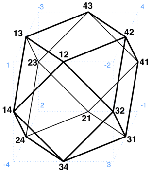
Figure 1. The root polytope ${\mathcal{P}}_{A_{3}}$.

For a finite set $A$ let $\Delta_{A}$ be the standard $(|A|-1)$-dimensional simplex whose vertices are the unit vectors in ${\mathbb{R}}^{|A|}$. The following proposition summarizes several useful properties of the root polytope $P_{A_{n}}$.

Proposition 8.

The polytope ${\mathcal{P}}_{A_{n}}$ is an $n$-dimensional polytope in ${\mathbb{R}}^{n+1}$ which is contained in the hyperplane $H_{0}=\{{\mathbf{x}}\in{\mathbb{R}}^{n+1}:\sum_{i=0}^{n}x_{i}=0\}$. It has $(n-1)n(n+1)$ edges, which are of the form ${\mathbf{v}}_{ij}{\mathbf{v}}_{ik}$ and ${\mathbf{v}}_{ik}{\mathbf{v}}_{jk}$ for $i,j,k$ distinct. It has $2^{n+1}-2$ facets, which can be labelled by the proper subsets $S$ of $[0,n]:=\{0,1,\ldots,n\}$. The facet ${\mathcal{F}}_{S}$ is defined by the hyperplane

$$H_{S}:=\left\{{\mathbf{x}}\in{\mathbb{R}}^{n+1}:\,\,\sum_{i\in S}x_{i}=1\right\},$$

and it is congruent to the product of simplices $\Delta_{S}\times\Delta_{T}$, where $T=[0,n]-S$. The only lattice points in ${\mathcal{P}}_{A_{n}}$ are its vertices and the origin.

Proof.

The first statement is clear. The edges ${\mathbf{v}}_{ij}{\mathbf{v}}_{ik}$ and ${\mathbf{v}}_{ik}{\mathbf{v}}_{jk}$ are maximized by the functionals $x_{i}-x_{j}-x_{k}$ and $x_{i}+x_{j}-x_{k}$, respectively. To see that we cannot have an edge whose vertices are ${\mathbf{v}}_{ij}$ and ${\mathbf{v}}_{kl}$ with $i,j,k,l$ distinct, note that ${\mathbf{v}}_{ij}+{\mathbf{v}}_{kl}={\mathbf{v}}_{il}+{\mathbf{v}}_{kj}$; so any linear functional $f$ satisfies that $f({\mathbf{v}}_{ij})+f({\mathbf{v}}_{kl})=f({\mathbf{v}}_{il})+f({\mathbf{v}}_{kj})$ and cannot be maximized precisely at this presumed edge. Similarly, we cannot have an edge with vertices ${\mathbf{v}}_{ij}$ and ${\mathbf{v}}_{ki}$ since ${\mathbf{v}}_{ij}+{\mathbf{v}}_{ki}={\mathbf{v}}_{lj}+{\mathbf{v}}_{kl}$ for any $l$ distinct from $i,j,k$.

The vertices of ${\mathcal{P}}_{A_{n}}$ that lie on $H_{S}$ are those of the form ${\mathbf{v}}_{ij}$ for $i\in S$ and $j\notin T$; these clearly form a polytope isomorphic to the product of simplices $\Delta_{S}\times\Delta_{T}$. Since this polytope has codimension one in ${\mathcal{P}}_{A_{n}}$, it is indeed a facet. Now consider any facet ${\mathcal{F}}$ of ${\mathcal{P}}_{A_{n}}$ defined by a functional $f$. By the previous paragraph, every edge of ${\mathcal{F}}$ has direction of the form ${\mathbf{e}}_{i}-{\mathbf{e}}_{j}$ for some $i\neq j$; and the fact that this edge lies on ${\mathcal{F}}$ implies that $f({\mathbf{e}}_{i})=f({\mathbf{e}}_{j})$. Doing this for $n-1$ linearly independent edges of ${\mathcal{F}}$, we get $n-1$ independent equalities among the $f({\mathbf{e}}_{i})$, showing that there can only be two different values among $f({\mathbf{e}}_{0}),\ldots,f({\mathbf{e}}_{n})$. Since ${\mathcal{P}}_{A_{n}}$ lies on $H_{0}$ we can assume that the smaller value is $0$, and by rescaling we can make the larger value $1$. It follows that ${\mathcal{F}}$ is one of the facets already described.

Since ${\mathcal{P}}_{A_{n}}$ is contained in the sphere of radius $\sqrt{2}$ centered at $0$, it can only contain lattice points of the form $0,\pm{\mathbf{e}}_{i}$, or $\pm{\mathbf{e}}_{i}\pm{\mathbf{e}}_{j}$. Of these, the only ones on the hyperplane $H_{0}$ are the origin and the vertices of ${\mathcal{P}}_{A_{n}}$. ∎

Now we will construct a specific unimodular triangulation of ${\mathcal{P}}_{A_{n}}$ (equivalently, of $\operatorname{cone}(M_{A_{n}}^{\prime})$). The combinatorial structure of this triangulation will allow us to enumerate its faces.

Proposition 9.

[13] The matrix $M_{A_{n}}$ is totally unimodular; i.e., every square submatrix of $M_{A_{n}}$ has determinant $0,\,+1$, or $-1$. The same is true for $M_{A_{n}}^{\prime}$.

Corollary 10.

Let ${\mathcal{T}}$ be an arbitrary triangulation of the boundary of ${\mathcal{P}}_{A_{n}}$. Coning over ${\mathcal{T}}$ from the origin gives rise to a unimodular triangulation of ${\mathcal{P}}_{A_{n}}\cup 0$.

In light of Corollary 10 we need a triangulation of the boundary of ${\mathcal{P}}_{A_{n}}$. Such a triangulation will be obtained as a pulling triangulation, also known as a reverse lexicographic triangulation. Let ${\mathcal{A}}=\{a_{1},\ldots,a_{r}\}$ be a collection of points in ${\mathbb{R}}^{n}$, totally ordered by $a_{1}\prec a_{2}\prec\dots\prec a_{r}$, and let ${\mathcal{P}}_{{\mathcal{A}}}$ be the convex hull of ${\mathcal{A}}$. We define the faces of ${\mathcal{A}}$ to be the subsets of ${\mathcal{A}}$ that lie on the faces of the polytope ${\mathcal{P}}_{{\mathcal{A}}}$.

Definition 2.

A pulling triangulation $\Gamma_{pull}({\mathcal{A}})$ is defined recursively as follows:

• If ${\mathcal{A}}$ is affinely independent, then $\Gamma_{pull}({\mathcal{A}})=\{{\mathcal{A}}\}.$

• Otherwise,

  $$\Gamma_{pull}({\mathcal{A}})=\bigcup_{\mathcal{F}}\{\{a_{1}\}\cup\,{\mathcal{G}}:{\mathcal{G}}\in\Gamma_{pull}({\mathcal{F}})\}$$

  where the union is taken over all facets ${\mathcal{F}}$ of ${\mathcal{A}}$ not containing $a_{1}.$

Definition 3.

The staircase triangulation $\Gamma$ of ${\mathcal{P}}_{A_{n}}$ is the pulling triangulation of the set ${\mathcal{M}}_{A_{n}}\cup{\mathbf{0}}$ under the ordering

$${\mathbf{0}}\prec{\mathbf{v}}_{01}\prec{\mathbf{v}}_{02}\prec\cdots\prec{\mathbf{v}}_{0,n}\prec{\mathbf{v}}_{10}\prec{\mathbf{v}}_{12}\prec\cdots\prec{\mathbf{v}}_{1,n}\prec\cdots\prec{\mathbf{v}}_{n,0}\prec{\mathbf{v}}_{n,n-1}$$

Since the origin is pulled first, $\Gamma$ is the cone over a triangulation of the boundary of ${\mathcal{P}}_{A_{n}}$, and it suffices to understand how each facet $\Delta_{S}\times\Delta_{T}$ of ${\mathcal{P}}_{A_{n}}$ gets triangulated. Fortunately, the restriction of $\Gamma$ to this facet is the well-understood staircase triangulation of a product of two simplices [10]. The vertices of $\Delta_{S}\times\Delta_{T}$ correspond to the entries of the $S\times T$ submatrix of the matrix ${\mathcal{V}}_{n}$, and the maximal simplices of the staircase triangulation of this facet correspond to the “staircase” paths that go from the top left to the bottom right corner of this submatrix taking steps down and to the right. We will let $\Gamma=\Gamma({\mathcal{P}}_{A_{n}}),\partial\Gamma=\Gamma(\partial{\mathcal{P}}_{A_{n}}),$ and $\Gamma(\Delta_{S}\times\Delta_{T})$ denote the staircase triangulation of ${\mathcal{P}}_{A_{n}}$, its restriction to the boundary $\partial{\mathcal{P}}_{A_{n}}$, and its restriction to the facet $\Delta_{S}\times\Delta_{T}$, respectively.

Example 2.

The facet ${\mathcal{F}}_{046}\cong\Delta_{046}\times\Delta_{1235}$ of the root polytope ${\mathcal{P}}_{A_{6}}$ is the convex hull of the vertices in the following submatrix of ${\mathcal{V}}_{6}$:

$$\left(\begin{array}[]{cccc}{\mathbf{v}}_{01}&{\mathbf{v}}_{02}&{\mathbf{v}}_{03}&{\mathbf{v}}_{05}\\ {\mathbf{v}}_{41}&{\mathbf{v}}_{42}&{\mathbf{v}}_{43}&{\mathbf{v}}_{45}\\ {\mathbf{v}}_{61}&{\mathbf{v}}_{62}&{\mathbf{v}}_{63}&{\mathbf{v}}_{65}\\ \end{array}\right).$$

There are $10$ maximal cells in $\Gamma(\Delta_{046}\times\Delta_{1235})$, corresponding to the ${5\choose 2}=10$ staircase paths from ${\mathbf{v}}_{01}$ to ${\mathbf{v}}_{65}$. The simplex with vertices $\{{\mathbf{v}}_{01},{\mathbf{v}}_{02},{\mathbf{v}}_{42},{\mathbf{v}}_{43},{\mathbf{v}}_{45},{\mathbf{v}}_{65}\}$ is one of these cells; it corresponds to the staircase

$$\left[\begin{array}[]{cccc}{\mathbf{v}}_{01}&{\mathbf{v}}_{02}&-&-\\ -&{\mathbf{v}}_{42}&{\mathbf{v}}_{43}&{\mathbf{v}}_{45}\\ -&-&-&{\mathbf{v}}_{65}\\ \end{array}\right].$$

The facet $\Delta_{S}\times\Delta_{T}$ is subdivided into ${|S|+|T|-2\choose|S|-1}$ simplices. It follows that the number of full-dimensional simplices of $\Gamma$ is

$$f_{n}(\Gamma)=f_{n-1}(\partial\Gamma)=\sum_{k=1}^{n}{n+1\choose k}{n-1\choose k-1}={2n\choose n}.$$

The following gives a characterization of all faces of $\partial\Gamma$.

Proposition 11.

The $(m-1)$-dimensional faces of the staircase triangulation $\partial\Gamma$ are given by subsets $\{v_{i_{1}j_{1}},\ldots,v_{i_{m}j_{m}}\}$ of the set of vertices such that:

1. $0\leq i_{1}\leq i_{2}\leq\ldots\leq i_{m}\leq n$ and $\,0\leq j_{1}\leq j_{2}\leq\ldots\leq j_{m}\leq n$,

2. $(i_{s},j_{s})\neq(i_{t},j_{t})$ for $s\neq t$, and

3. $i_{s}\neq j_{t},$  $1\leq s,t\leq m$.

Proof.

This is straightforward from the definitions. The third condition guarantees that ${\mathbf{v}}_{i_{1}j_{1}},\ldots,{\mathbf{v}}_{i_{m}j_{m}}$ are vertices of some (not necessarily unique) facet $\Delta_{S}\times\Delta_{T}$, while the first two conditions guarantee that they form a subset of some staircase path in the corresponding $S\times T$ submatrix of ${\mathcal{V}}_{n}$. ∎

In the matrix ${\mathcal{V}}_{n}$, we can see a face as a sequence of positions that (1) moves weakly southeast, (2) never stagnates, and (3) never uses a row and a column of the same label. This is illustrated in Figure 2.

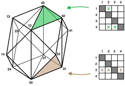
Figure 2. The staircase triangulation of the root polytope ${\mathcal{P}}_{A_{3}}$.

Theorem 12.

The $f$-vector of the reverse lexicographic triangulation $\partial\Gamma$ of the boundary of $P_{A_{n}}$ is given by

$$f_{m-1}(\partial\Gamma)=f_{m}(\Gamma)=\binom{n+m}{m,m,n-m}$$

for $0\leq m\leq n$.

Proof.

The problem of counting the $m$-faces of $\Gamma(P_{A_{n}})$ has been reduced to counting the possible choices for indices $(i_{1},j_{1}),\ldots,(i_{m},j_{m})$ that meet the conditions in Proposition 11. We find it convenient to view these as $m$ positions in the matrix ${\mathcal{V}}_{n}$.

Consider the choices that occupy exactly $a$ columns and $b$ rows. There are ${n+1\choose a,b,n+1-a-b}$ choices of rows and columns satisfying condition (3). Once we have chosen these, let us focus our attention on the $a\times b$ submatrix that remains; condition (3) guarantees that there are no zero entries in this matrix. Inside this submatrix, the vertices $(i_{1},j_{1}),\ldots,(i_{m},j_{m})$ form a path that never moves up or to the left and touches every row and column. This path must go from the top left to the bottom right corner of the submatrix using the steps $(1,0),(0,-1)$, and $(1,-1)$. The total number of steps is $m-1$ and the distances covered by the path in the horizontal and vertical directions are $b-1$ and $a-1$, respectively. Therefore, the number of steps of the form $(1,0),(0,-1)$, and $(1,-1)$ must be $m-a,m-b,$ and $a+b-m-1$, respectively. There are ${m-1\choose m-a,m-b,a+b-m-1}$ paths of this form.

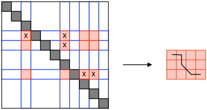
Figure 3. Going from the label of a cell of $\partial\Gamma$ to a path in a rectangle with steps $(1,0),(0,-1)$ and $(1,-1)$.

Figure 3 shows how to convert a partial staircase into a path from the top left to the bottom right corner of a rectangle, using steps of the form $(1,0),(0,-1)$ and $(1,-1)$. First we select the rows and columns used by the partial staircase, and delete all the other ones. The cells of the staircase form a path in the resulting rectangle.

It follows that

$$f_{m-1}(\partial\Gamma) = \sum_{a,b}{n+1\choose a,b,n+1-a-b}{m-1\choose m-a,m-b,a+b-m-1}$$

$${n+m\choose n+1}f_{m-1}(\partial\Gamma) = \sum_{a,b}{n+m\choose n+1}{n+1\choose a,b,n+1-a-b}{m-1\choose m-a,m-b,a+b-m-1}$$

$$= \sum_{a,b}{n+m\choose a,b,n+1-a-b,m-a,m-b,a+b-m-1}$$

$$= \sum_{a,b}{n+m\choose m,m,n-m}{m\choose a}{m\choose b}{n-m\choose n+1-a-b}$$

$$= {n+m\choose m,m,n-m}{n+m\choose n+1}$$

as desired. ∎

Theorem 13.

The coordinator polynomial for the growth series of the lattice $A_{n}$ generated as a monoid by ${\mathcal{M}}_{A_{n}}=\{{\mathbf{e}}_{i}-{\mathbf{e}}_{j},:\,0\leq i,j\leq n+1\,\,\text{with}\,\,i\neq j\}$ is

$$h_{A_{n}}(x)=\sum_{k=0}^{n}{n\choose k}^{2}x^{k}.$$

Proof.

We first compute $h_{\partial\Gamma}(x)$. By definition $h_{\partial\Gamma}(x+1)=f_{\partial\Gamma}(x)$, which is

$$\sum_{m=0}^{n}{n+m\choose m,m,n-m}x^{n-m}=\sum_{l=0}^{n}{n\choose l}{2n-l\choose n}x^{l} = \sum_{l=0}^{n}\sum_{k=l}^{n}{n\choose l}{n\choose k}{n-l\choose n-k}x^{l}=$$

$$\sum_{l=0}^{n}\sum_{k=l}^{n}{n\choose k}^{2}{k\choose l}x^{l}=\sum_{k=0}^{n}\sum_{l=0}^{k}{n\choose k}^{2}{k\choose l}x^{l} = \sum_{k=0}^{n}{n\choose k}^{2}(x+1)^{k}.$$

This shows that $h_{\partial\Gamma}(x)=\sum_{k=0}^{n}{n\choose k}^{2}x^{k}$, and since this polynomial is palindromic we get $h_{A_{n}}(x)=x^{n}h_{\partial\Gamma}(x^{-1})=h_{\partial\Gamma}(x)$. ∎

4. The Lattice $C_{n}$

The root lattice $C_{n}\subset{\mathbb{R}}^{n}$ is defined by $C_{n}:=\{{\mathbf{x}}\in{\mathbb{Z}}^{n}:\sum_{i}x_{i}\,\,\text{is even}\}.$

Proposition 14.

The root lattice $C_{n}$ is a rank $n$ lattice generated as a monoid by the set ${\mathcal{M}}_{C_{n}}=\{\pm 2{\mathbf{e}}_{i}:1\leq i\leq n\,;\,\pm{\mathbf{e}}_{i}\pm{\mathbf{e}}_{j}:1\leq i\neq j\leq n\}$.

Proof.

Consider any ${\mathbf{x}}\in C_{n}$. By subtracting from it the appropriate nonnegative multiples of $2{\mathbf{e}}_{i}$ or $-2{\mathbf{e}}_{i}$, we obtain a vector ${\mathbf{y}}\in C_{n}$ where each $y_{i}$ equals $0$ or $1$. The number of coordinates of ${\mathbf{y}}$ equal to $1$ is even, so ${\mathbf{y}}$ is a sum of vectors of the form ${\mathbf{e}}_{i}+{\mathbf{e}}_{j}$ with $i\neq j$. ∎

As in the earlier section, we define ${\mathcal{P}}_{C_{n}}=\operatorname{conv}({\mathcal{M}}_{C_{n}})$. The root polytope ${\mathcal{P}}_{C_{n}}$ is the cross polytope (which we will define next) dilated by a factor of two, ${\mathcal{P}}_{C_{n}}=2\Diamond_{n}$.

Definition 4.

The crosspolytope $\Diamond_{n}$ in ${\mathbb{R}}^{n}$ is given by the facet and vertex descriptions

$$\Diamond_{n}:=\left\{{\mathbf{x}}\in{\mathbb{R}}^{n}:\sum_{i=1}^{n}|x_{i}|\leq 1\right\}=\operatorname{conv}(\{{\mathbf{e}}_{1},-{\mathbf{e}}_{1},\dots,{\mathbf{e}}_{n},-{\mathbf{e}}_{n}\}).$$

Remark.

In the rest of this section we will compute the growth series of ${\mathcal{L}}_{{\mathcal{M}}_{C_{n}}}$ essentially by considering lattice points in the integer dilates of ${\mathcal{P}}_{C_{n}}$. However, when we say “lattice points” or “unimodular triangulation,” we mean these words with respect to the lattice ${\mathcal{L}}_{{\mathcal{M}}_{C_{n}}}$. For instance, in this sense, the only interior lattice point of ${\mathcal{P}}_{C_{n}}$ is the origin.

In Section 5.4 we will derive a unimodular triangulation of ${\mathcal{P}}_{C_{n}}$ from a triangulation of the root polytope ${\mathcal{P}}_{D_{n}}$, and use it to give a proof of Theorem 2 in the $C_{n}$ case. Such a triangulation is obtained from a triangulation of the facets of ${\mathcal{P}}_{D_{n}}$ by forming the cone of this boundary triangulation from the origin. One can also construct a specific pulling triangulation where the origin is pulled first; for the details we refer the reader to Section 5.2 in [13]. Here we give a different proof; we start by giving a simple description of the lattice points on the faces of the root polytope ${\mathcal{P}}_{C_{n}}$.

Proposition 15.

The set of lattice points on any $(k-1)$-face of ${\mathcal{P}}_{C_{n}}$ for $k=0,\ldots,n$ is affinely isomorphic to the set of lattice points in the simplex

$$V(2,k):=\left\{{\mathbf{u}}\in{\mathbb{Z}}_{\geq 0}^{k}\,:\>u_{1}+u_{2}+\cdots+u_{k}=2\right\}.$$

Proof.

This is immediate from the fact that crosspolytopes are regular and simplicial. ∎

The Hilbert series of $K[V(2,k)]$ is given in [11, Corollary 2.6] as

$$H(K[V(2,k)],x)=\frac{h_{k}(x)}{(1-x)^{k}}=\frac{\sum_{i=0}^{k}{k\choose 2i}x^{i}}{(1-x)^{k}}.$$

Now we can compute the growth series of $C_{n}$ as an inclusion-exclusion count of Hilbert series of above kind for all dimensions, namely

$$\sum_{j=0}^{n}(-1)^{n-j}f_{j-1}\frac{h_{j}(x)}{(1-x)^{j}}$$

where $f_{j-1}$ is the number of $(j-1)$-dimensional faces of the cross polytope $\Diamond_{n}$. Using the duality between the cross polytope and the $n$-dimensional hypercube we know that $f_{j-1}={n\choose j}2^{j}$. Substituting this in the above series and writing with a common denominator we get

$$\frac{1}{(1-x)^{n}}\sum_{j=0}^{n}(-1)^{n-j}(1-x)^{n-j}{n\choose n-j}2^{j}\sum_{i=0}^{j}{j\choose 2i}x^{i}.$$

The numerator of this series is the coordinator polynomial we are after, and note that this polynomial consists of the whole power terms of

$$\sum_{j=0}^{n}(-1)^{n-j}(1-x)^{n-j}{n\choose n-j}2^{j}(1+\sqrt{x})^{j}.$$

Using the binomial theorem, the above polynomial is equal to $((x-1)+(2+2\sqrt{x}))^{n}=(1+\sqrt{x})^{2n}$. This leads us to our main theorem in this section.

Theorem 16.

The coordinator polynomial for the lattice $C_{n}$ generated as a monoid by the standard generators ${\mathcal{M}}_{C_{n}}=\{\pm{\mathbf{e}}_{i}\pm{\mathbf{e}}_{j}:1\leq i,j\leq n\}$ is given by

$$h_{C_{n}}(x)=\sum_{k=0}^{n}\binom{2n}{2k}x^{k}.$$

From this, we use the method of Theorem 13 to extract the corresponding $f$-polynomial

$$f_{C_{n}}(x)=\sum_{m=0}^{n}\frac{n\,2^{2m}}{n+m}\binom{n+m}{2m}x^{n-m}$$

proving the statement in Theorem 1.

5. The lattice $D_{n}$

The root lattice $D_{n}$ is defined by $D_{n}:=\{x\in\mathbbm{Z}^{n}:\sum_{i}x_{i}\text{ is even}\}$. Note that this lattice is the same as $C_{n}$. The only difference is in the set of generators.

Proposition 17.

The root lattice $D_{n}$ is generated by ${\mathcal{M}}_{D_{n}}=\{\pm{\mathbf{e}}_{i}\pm{\mathbf{e}}_{j}:1\leq i\neq j\leq n\}$ as a monoid. $\Box$

Proof.

Observe that $2{\mathbf{e}}_{i}=({\mathbf{e}}_{i}+{\mathbf{e}}_{j})+({\mathbf{e}}_{i}-{\mathbf{e}}_{j})$ and invoke Proposition 14. ∎

Let $\Delta_{2,n}=\operatorname{conv}\{{\mathbf{e}}_{i}+{\mathbf{e}}_{j}:1\leq i\neq j\leq n\}$ be the $(n-1)$-dimensional second hypersimplex in $\mathbbm{R}^{n}$.

Proposition 18.

The root polytope ${\mathcal{P}}_{D_{n}}=\operatorname{conv}{\mathcal{M}}_{D_{n}}$ has dimension $n$, $2n(n-1)$ vertices, $2^{n}$ hypersimplex facets $\Delta_{2,n}$, and $2n$ cross-polytope facets $\Diamond_{n-1}$.

Proof.

The first two statements are immediate. Next, we claim that the facet-defining inequalities come in two families, $\sum_{i=1}^{d}\sigma_{i}x_{i}\leq 2$ and $\sigma_{i}x_{i}\leq 1$, where $\sigma_{i}\in\{\pm 1\}$. To verify that they all describe facets of ${\mathcal{P}}_{D_{n}}$, it suffices to consider the case $\sigma_{i}=1$ for all $i$. The vertices in ${\mathcal{P}}_{D_{n}}$ with $x_{1}+\dots+x_{d}=2$ are just the permutations of $(1,1,0,\dots,0)$, which by definition are the vertices of $\Delta_{2,n}$. For the second family, we can additionally assume $i=1$, so that the set of vertices in ${\mathcal{P}}_{D_{n}}$ satisfying $x_{1}=1$ is exactly $(1,\pm 1,0,\dots,0),\dots,(1,0,\dots,0,\pm 1)$, the set of vertices of an $(n-1)$-dimensional cross-polytope $\Diamond_{n-1}$.

Convincing ourselves that we didn’t miss any facets of ${\mathcal{P}}_{D_{n}}$ can be done directly, but it also follows quickly using the fact that ${\mathcal{P}}_{D_{n}}$ arises from the Wythoff construction [8] associated to the following diagram:

We can read off the facets of ${\mathcal{P}}_{D_{n}}$ from this diagram by forming connected subgraphs with $n-1$ vertices that contain the “ringed” node. There are exactly two such subgraphs, corresponding to cross-polytopes $\Diamond_{n-1}$ and hypersimplices $\Delta_{n,2}$, respectively. The counting method detailed in [8] now assures us that we have accounted for all facets of ${\mathcal{P}}_{D_{n}}$. ∎

To calculate the generating function of the $f$-vector of our triangulation $\operatorname{triang}\partial{\mathcal{P}}_{D_{n}}$ of the boundary of ${\mathcal{P}}_{D_{n}}$, we split

$$\operatorname{triang}\partial{\mathcal{P}}_{D_{n}}\ =\ \operatorname{triang}{\mathcal{P}}_{D_{n},\operatorname{total}\operatorname{int}\Diamond_{n-1}}\ \cup\ \operatorname{triang}{\mathcal{P}}_{D_{n},\operatorname{total}\Delta_{2,n}}$$

into the disjoint union of all faces in the interior of a cross-polytope facet, respectively all faces contained in a hypersimplex facet.

5.1. Triangulating the cross-polytope facets

We start with $\operatorname{triang}{\mathcal{P}}_{D_{n},\operatorname{total}\operatorname{int}\Diamond_{n-1}}$. Since cross-polytopes are simplicial, the way in which we choose to triangulate them will not affect the triangulations of the hypersimplex facets, and the entire boundary of the cross-polytope will be contained in the triangulation. More precisely, there are $\binom{m}{k+1}2^{k+1}$ faces of dimension $k$ in the boundary complex of an $m$-dimensional cross-polytope; we include the empty face by allowing $k=-1$. These numbers assemble into the generating function

$$f_{\partial\Diamond_{m}}(x)\ =\ \sum_{k=-1}^{m-1}\binom{m}{k+1}2^{k+1}x^{k}\ =\ \frac{1}{x}\sum_{k=0}^{m}\binom{m}{k}(2x)^{k}\ =\ \frac{(1+2x)^{m}}{x}.$$

We now extend the boundary to a unimodular triangulation of $\Diamond_{n-1}$. However, just as in Section 4, we must be careful to only use lattice points from our root lattice; for $D_{n}$ this means that we must exclude the centroid of each $\Diamond_{n-1}$ from the triangulation, because it has odd coordinate sum.

Instead, setting $m=n-1$, we need to triangulate the interior of $\Diamond_{m}$ without using any new vertices. There is still not much choice in the matter, since all such triangulations are combinatorially isomorphic; they are determined by the choice of a diagonal connecting two opposite vertices, say $v_{2m-1}$ and $v_{2m}$. The faces of the triangulation of $\Diamond_{m}$ are then either faces of the boundary $\partial\Diamond_{m}$, or joins $\{v_{2m-1},v_{2m}\}\star F$, where $F$ is a face of the “equatorial” $\partial\Diamond_{m-1}$. Here we include the case $F=\emptyset$, which we take to yield the diagonal $\operatorname{conv}\{v_{2m-1},v_{2m}\}$ itself. However, we exclude the faces in the boundary $\partial\Diamond_{m}$ from our count, because these will be included in the generating function of the triangulation of the hypersimplex facets. Thus, the $f$-vector of interior faces of our triangulation of $\Diamond_{n-1}$ is

$$f_{\operatorname{int}\Diamond_{n-1}}(x)\ =\ x^{2}f_{\partial\Diamond_{n-2}}(x)\ =\ (1+2x)^{n-2},$$

and these values assemble into the following generating function for the number of interior faces of $\Diamond_{n-1}$:

$$F_{\operatorname{int}\Diamond_{n-1}}(z,x)\ =\ \sum_{n\geq 2}f_{\operatorname{int}\Diamond_{n-1}}(x)z^{n}\ =\ \sum_{n\geq 2}x(1+2x)^{n-2}z^{n}\ =\ -\frac{xz^{2}}{2xz+z-1}.$$

Because ${\mathcal{P}}_{D_{n}}$ has $2n$ cross-polytope facets, we obtain the total count of such interior faces as

$$F_{D_{n},\operatorname{total}\operatorname{int}\Diamond_{n-1}}(z,x)\ =\ 2z\frac{\partial}{\partial z}F_{\operatorname{int}\Diamond_{n-1}}(z,x)\ =\ -\frac{2xz^{2}(2xz+z-2)}{(2xz+z-1)^{2}}.$$

For the $f$-vector, this means

$$f_{k}^{\operatorname{total}\operatorname{int}\Diamond_{n-1}}\ =\ n\,2^{k}\binom{n-2}{k-1}.$$

Note that there is no double-counting here, because the interior faces of the triangulations of the cross-polytope facets are disjoint.

5.2. Triangulating the hypersimplex facets

Our next job is to calculate the number $f_{k}(D_{n},\operatorname{total}\Delta_{2,n})$ of $k$-dimensional faces of a unimodular triangulation of the hypersimplex facets of ${\mathcal{P}}_{D_{n}}$.

The unimodular triangulation of the hypersimplex $\Delta_{2,n}$ that we will use has an interesting history. Two such triangulations were constructed independently by Stanley [14] in 1977 and by Sturmfels [16] in 1996. However, in 2006, Lam and Postnikov [12] showed that these triangulations are in fact the same, and gave two more independent descriptions.

Let $f_{k}^{(n)}$ count the number of $k$-faces of this “standard” triangulation of the $(n-1)$-dimensional hypersimplex $\Delta_{2,n}$. These numbers were calculated by Lam and Postnikov, and are given implicitly in [12, Remark 5.4] via the generating function

$$F_{\Delta}(z,x) = \sum_{n\geq 2}z^{n}\sum_{k=0}^{n-1}f_{k}^{(n)}x^{k}$$

$$= \frac{z^{2}}{1-z}\cdot\frac{1+(1+x)z(z+x-2)}{(xz+z-1)^{2}\big{(}(1+x)z(z-2)+1\big{)}}$$

$$= z^{2}+(3+3x+x^{2})z^{3}+(6+13x+12x^{2}+4x^{3})z^{4}+O(z^{5}).$$

Some remarks are in order here: First, we have removed a factor ‘$x$’ from the formula in [12, Remark 5.4], because Lam and Postnikov’s normalization of the $f$-vector is different from ours. Secondly, in this subsection we do not include a count for the empty face in our generating functions, because we want to combine triangulations into larger ones, but prefer not to be bothered by the fact that each triangulation has a unique empty face; we will remedy this starting from Section 5.3. And finally, note that the $z^{2}$ term in the formula corresponds to the unique $0$-dimensional face of $\Delta(2,2)$.

These remarks out of the way, we count the number of $(k\geq 0)$-dimensional faces of $\operatorname{triang}{\mathcal{P}}_{D_{n},\operatorname{total}\Delta_{2,n}}$ by an inclusion-exclusion argument, making use of the following two facts: For $k\neq 1$, each $k$-dimensional face of a hypersimplex is again a hypersimplex; and for $n\geq 3$ each hypersimplex facet of ${\mathcal{P}}_{D_{n}}$ is adjacent to exactly $n$ other hypersimplex facets. (There is an additional oddity for $n=3$, in that it remains true that each of the 8 triangles $\Delta(3,2)$ in ${\mathcal{P}}_{D_{3}}$ is adjacent to exactly $3$ other ones, but the adjacency happens via vertices, not codimension 1 faces.)

The count must start out $2^{n}f_{k}^{(n)}$, but then we have overcounted the $k$-faces in the intersections of two hypersimplex facets. For each such intersection, we must subtract $f_{k}^{(n-1)}$, so it remains to calculate the number of such adjacencies of hypersimplex facets. Without loss of generality, we can assume one of the hypersimplex facets to lie in the hyperplane $\sum_{i=1}^{n}x_{i}=\langle a,x\rangle=2$, where $a=(1,\dots,1)$ is the all-1 vector. This facet $F$ is adjacent to $n$ other hypersimplex facets $F_{1},\dots,F_{n}$, namely the ones defined by the normal vectors obtained from $a$ by changing exactly one 1 to $-1$. A normal vector that selects the $(n-2)$-dimensional hypersimplex $F\cap F_{j}$ is obtained from $a$ by setting the $j$-th entry to $0$.

For $i$ with $1\leq i\leq n-2$, any $(n-i)$-dimensional hypersimplex that is the intersection of $i$ hypersimplex facets of ${\mathcal{P}}_{D_{n}}$ lies in the hyperplane $\langle a^{\prime},x\rangle=2$, where $a^{\prime}$ is a vector with $i-1$ entries ‘$0$’ and the remaining $n-i+1$ entries either ‘$+1$’ or ‘$-1$’. Since there are $\binom{n}{i-1}2^{n-i+1}$ such vectors, we obtain

$$f_{k}(D_{n},\operatorname{total}\Delta_{2,n}) = \sum_{i=1}^{n-2}(-1)^{i-1}\binom{n}{i-1}2^{n-i+1}f_{k}^{(n-i+1)}$$

$$= \sum_{j\geq 0}(-1)^{j}\binom{n}{j}2^{n-j}f_{k}^{(n-j)}.$$

Note that the last sum only runs up to $n-k$ because $f_{k}^{(l)}=0$ for $k>l$.

Let’s discuss some special cases: The sum (5.2) is also valid for $n=3$; for $i\geq n$ because $f^{(l)}_{k}=0$ for $l\leq 1$ and all $k$; and for $i=n-1$ (the case of edges) because $f^{(2)}_{0}=1$ is the only nonzero value of $f^{(2)}$, so that $f_{0}(D_{n},\operatorname{total}\Delta_{2,n})$ is the only affected term; but the number of vertices works out correctly. This comes about because $f_{0}(\Delta_{2,n})=\binom{n}{2}$, so that

$$f_{0}(D_{n},\operatorname{total}\Delta_{2,n})\ =\ \sum_{j\geq 0}(-1)^{j}\binom{n}{j}2^{n-2}\binom{n-j}{2}\ =\ 2n(n-1),$$

the correct number of vertices.

We proceed to calculate the corresponding generating functions:

$$f_{D_{n},\operatorname{total}\Delta_{2,n}}(x) = \sum_{k=0}^{n-1}f_{k}(D_{n},\operatorname{total}\Delta_{2,n})x^{k}$$

$$= \sum_{i=0}^{n-1}(-1)^{i}\binom{n}{i}2^{n-i}\sum_{k=0}^{n-i}f_{k}^{(n-i)}x^{k}$$

$$= \sum_{i=0}^{n-1}(-1)^{i}\binom{n}{i}2^{n-i}f^{(n-i)}(x)$$

$$= (-1)^{n}\sum_{i=1}^{n}(-2)^{i}\binom{n}{i}f^{(i)}(x),$$

and

$$F_{D_{n},\operatorname{total}\Delta_{2,n}}(z,x) = \sum_{n\geq 2}f_{D_{n},\operatorname{total}\Delta_{2,n}}(x)z^{n}$$

$$= \sum_{i\geq 1}(-2)^{i}f^{(i)}(x)\sum_{n\geq i}(-z)^{n}\binom{n}{i}$$

$$= \sum_{i\geq 1}\frac{(2z)^{i}}{(1+z)^{i+1}}f^{(i)}(x)$$

$$= \frac{1}{1+z}\sum_{i\geq 1}\left(\frac{2z}{1+z}\right)^{i}f^{(i)}(x)$$

$$= \frac{1}{1+z}F_{\Delta}\left(\frac{2z}{1+z},x\right)$$

$$= \frac{4z^{2}}{(z-1)^{2}-4xz}\left(\frac{2xz(x+1)}{(2xz+z-1)^{2}}-\frac{1}{z-1}\right),$$

where $F_{\Delta}(z,x)=\sum_{i\geq 0}f^{(i)}(x)z^{i}$ is the generating function of the $f$-vectors of triangulations of the second hypersimplex from (5.2); note that $f^{(0)}(x)=f^{(1)}(x)=0$.

5.3. The total generating function

It remains to combine the two previous generating functions:

$$F_{\operatorname{triang}\partial{\mathcal{P}}_{D_{n}}}(z,x)\ =\ F_{D_{n},\operatorname{total}\operatorname{int}\Diamond_{n-1}}(z,x)+F_{D_{n},\operatorname{total}\Delta_{2,n}}(z,x)+\frac{1}{x}\sum_{n\geq 2}z^{n},$$

where the last term corresponds to a count for the empty face in each dimension. We could now extract the $f$-vector via a routine calculation; however, it will be easier to do this with the $h$-vector in hand.

For this, we form a unimodular triangulation $\Delta$ of the interior of ${\mathcal{P}}_{D_{n}}$ by coning over $\operatorname{triang}\partial{\mathcal{P}}_{D_{n}}$ from the origin. However, since we are interested only in the $h$-vector of the resulting triangulation, we can use two well-known properties of $h$-polynomials to simplify things. Namely, the $h$-polynomial $h_{\Delta_{1}\star\Delta_{2}}(x)=h_{\Delta_{1}\star\Delta_{2}}$ of the join of two simplicial complexes equals the product $h_{\Delta_{1}}h_{\Delta_{2}}$ of the individual $h$-polynomials; moreover, the $h$-polynomial of a point is $h_{\{0\}}=1$. Thus,

$$h_{\Delta}\ =\ h_{(\operatorname{triang}\partial{\mathcal{P}}_{D_{n}})\star\{0\}}\ =\ h_{\operatorname{triang}\partial{\mathcal{P}}_{D_{n}}},$$

and it suffices to calculate the $h$-polynomial corresponding to $\operatorname{triang}\partial{\mathcal{P}}_{D_{n}}$. For this, we need to re-index each polynomial

$$[z^{n}]F_{\operatorname{triang}\partial{\mathcal{P}}_{D_{n}}}(z,x)\ =\ \sum_{i=0}^{n}f_{i-1}x^{i-1}$$

to read instead $\sum_{i=0}^{n}f_{i-1}x^{n-i}$; we achieve this by setting

$$\widetilde{F}_{\operatorname{triang}\partial{\mathcal{P}}_{D_{n}}}(z,x)\ =\ \frac{1}{x}F_{\operatorname{triang}\partial{\mathcal{P}}_{D_{n}}}\bigg{(}zx,\frac{1}{x}\bigg{)}.$$

Since $h_{\Delta}(x)=f_{\Delta}(x-1)$, we obtain the generating function for the $h$-polynomials as

$$H_{D}(z,x) = \widetilde{F}_{\operatorname{triang}\partial{\mathcal{P}}_{D_{n}}}(z,x-1)$$

$$= z^{2}\frac{(1+x)^{2}-3(1+x)(1+x^{2})z+(3+x^{2})(1+3x^{2})z^{2}-(x-1)^{2}(1+x)(1+x^{2})z^{3}}{(xz+z-1)^{2}(1-2z(1+x)+z^{2}(x-1)^{2})}$$

$$= \frac{z^{2}}{2}\left(\frac{1}{\frac{1}{(\sqrt{x}-1)^{4}}-\frac{z}{(\sqrt{x}-1)^{2}}}+\frac{1}{\frac{1}{(\sqrt{x}+1)^{4}}-\frac{z}{(\sqrt{x}+1)^{2}}}\right)+\frac{2xz^{2}(xz+z-2)}{(xz+z-1)^{2}}$$

$$= \phantom{+{}}\big{(}1+2x+x^{2}\big{)}z^{2}$$

$$+\big{(}1+9x+9x^{2}+x^{3}\big{)}z^{3}$$

$$+\big{(}1+20x+54x^{2}+20x^{3}+x^{4}\big{)}z^{4}$$

$$+\big{(}1+35x+180x^{2}+180x^{3}+35x^{4}+x^{5}\big{)}z^{5}+O(z^{6}).$$

It is now straightforward to check that $H_{D}(z,x)=\sum_{n\geq 2}p_{n}(x)z^{n}$ is the generating function for Colin Mallows’s formula conjectured in Conway and Sloane [6]:

$$p_{n}(x)\ =\ \frac{(1+\sqrt{x})^{2n}+(1-\sqrt{x})^{2n}}{2}-2nx(1+x)^{n-2},$$

and from this we extract the $f$-vector stated in Theorem 1 without too much difficulty.

5.4. The growth series of $C_{n}$: reprise

We are now in a position to give a triangulation-theoretic derivation of the growth series of $C_{n}$. For this, notice from the description in Section 4 that the lattice points in ${\mathcal{P}}_{C_{n}}$ are the vertices of ${\mathcal{P}}_{D_{n}}$, together with the vertices of $2\Diamond_{n}$. We can therefore build a unimodular triangulation of the boundary of ${\mathcal{P}}_{C_{n}}$ by starting from our unimodular triangulation of ${\mathcal{P}}_{D_{n}}$. However, instead of triangulating the $2n$ cross-polytope facets, we cone over each such facet $F$ from the corresponding vertex $v_{F}$ of $2\Diamond_{n}$. By projecting $v_{F}$ into the barycenter of $F$, we see that counting the number of up to $(n-1)$-dimensional faces added by each coning operation amounts to counting the total number of interior faces in the triangulation of $\Diamond_{n-1}$ obtained by coning over the origin. These numbers, in turn, are encoded in the generating function

$$f_{\operatorname{int}(\{0\}\star\partial\Diamond_{n-1})}(x)\ =\ x\left(f_{\partial\Diamond_{n-1}}(x)-\frac{1}{x}\right)+1\ =\ (1+2x)^{n-1}.$$

As before, the faces corresponding to the cones over different cross-polytope facets are disjoint, so that their total number is counted by the generating function

$$F_{C_{n},\operatorname{total}\Diamond_{n-1}}(z,x)\ =\ 2z\frac{\partial}{\partial z}\sum_{n\geq 2}(1+2x)^{n-1}z^{n}\ =\ -\frac{2(2x+1)z^{2}(2xz+z-2)}{(2xz+z-1)^{2}}.$$

Combining generating functions as before, we obtain

$$(x-1)H_{C}(z,x) = \phantom{{}+{}}F_{C_{n},\operatorname{total}\Diamond_{n-1}}\left(z(x-1),\frac{1}{x-1}\right)$$

$${}+F_{D_{n},\operatorname{total}\Delta_{n,2}}\left(z(x-1),\frac{1}{x-1}\right)$$

$${}+(x-1)\sum_{n\geq 2}\left(z(x-1)\right)^{n}.$$

$$H_{C}(z,x) = z^{2}\frac{1+6x+x^{2}-(x-1)^{2}(x+1)z}{1-2(x+1)z+(x-1)^{2}z^{2}}$$

$$= \phantom{+{}}\big{(}1+6x+x^{2}\big{)}z^{2}$$

$$+\big{(}1+15x+15x^{2}+x^{3}\big{)}z^{3}$$

$$+\big{(}1+28x+70x^{2}+28x^{3}+x^{4}\big{)}z^{4}$$

$$+\big{(}1+45x+210x^{2}+210x^{3}+45x^{4}+x^{5}\big{)}z^{5}+O(z^{6}).$$

Again, it is easily checked that $H_{C}(z,x)=\sum_{n\geq 2}p_{n}(x)z^{n}$ with

$$p_{n}(x)\ =\ \sum_{k=0}^{n}\binom{2n}{2k}x^{k}.$$

References

- [1] M. Baake and U. Grimm, Coordination sequences for root lattices and related graphs, Z. Krist. 212 (1997), no. 4, 253–256.
- [2] Roland Bacher, Pierre de la Harpe, and Boris Venkov, Séries de croissance et séries d’Ehrhart associées aux réseaux de racines, C. R. Acad. Sci. Paris Sér. I Math. 325 (1997), no. 11, 1137–1142.
- [3] Matthias Beck and Serkan Hoşten, Cyclotomic polytopes and growth series of cyclotomic lattices, Math. Res. Lett. 13 (2006), no. 4, 607–622.
- [4] M. Benson, Growth series of finite extensions of are rational, Invent. Math. 73 (1983), no. 2, 251–269.
- [5] U. Betke and P. McMullen, Lattice points in lattice polytopes, Mh. Math. 99 (1985), 253–265.
- [6] John H. Conway and Neil J. A. Sloane, The cell structures of certain lattices, Miscellanea mathematica, Springer, Berlin, 1991, pp. 71–107.
- [7] by same author, Low-dimensional lattices. VII. Coordination sequences, Proc. Roy. Soc. London Ser. A 453 (1997), no. 1966, 2369–2389.
- [8] H. S. M. Coxeter, Regular polytopes, third ed., Dover Publications Inc., New York, 1973.
- [9] David Eisenbud, Commutative algebra,with a view toward algebraic geometry, Graduate Texts in Mathematics, vol. 150, Springer-Verlag, New York, 1995.
- [10] Israel M. Gelfand, Mikhail M. Kapranov, and Andrei V. Zelevinsky, Discriminants, resultants, and multidimensional determinants, Birkhäuser, 1994.
- [11] Mordechai Katzman, The Hilbert series of algebras of the Veronese type, Comm. Algebra 33 (2005), no. 4, 1141–1146.
- [12] T. Lam and A. Postnikov, Alcoved polytopes I, arXiv:math.CO/0501246v2, 2006.
- [13] Kimberly Seashore, Using polytopes to derive growth series for classical root lattices, Masters Thesis, San Francisco State University, 2007.
- [14] Richard Stanley, Eulerian partitions of a unit hypercube., Higher Comb., Proc. NATO Adv. Study Inst., Berlin (West) 1976, 49 (1977)., 1977.
- [15] by same author, Decompositions of rational convex polytopes, Annals of Discrete Math. 6 (1980), 333–342.
- [16] Bernd Sturmfels, Gröbner bases and convex polytopes, University Lecture Series, vol. 8, American Mathematical Society, Providence, RI, 1996.
- [17] Günter M. Ziegler, Lectures on polytopes, Graduate Texts in Mathematics, vol. 152, Springer-Verlag, New York, 1995.