QUANTUM TRACES IN QUANTUM TEICHMÜLLER THEORY

Abstract.

We prove that for the torus with one hole and $p\geqslant 1$ punctures and the sphere with four holes there is a family of quantum trace functions in the quantum Teichmüller space, analog to the non-quantum trace functions in Teichmüller space, satisfying the properties proposed by Chekhov and Fock in [3].

1. Introduction

The physicists L. Chekhov and V. Fock and, independently, R. Kashaev introduced a quantization of the Teichmüller space as an approach to quantum gravity in $2+1$ dimensions. A widespread philosophy in mathematics is that studying a space is the same as studying the algebra of functions on that space. The quantum Teichmüller space of Chekhov-Fock and Kashaev $\mathcal{T}_{S}^{q}$ is a certain non-commutative deformation of the algebra of rational functions on the usual Teichmüller space $\mathcal{T}(S)$. Namely, $\mathcal{T}_{S}^{q}$ depends on a parameter $q=e^{i\hbar}$ and converges to the algebra of functions on $\mathcal{T}(S)$ as $q\rightarrow 1$ or, equivalently as the Planck constant $\hbar\rightarrow 0$.

At this point in time, the quantum Teichmüller space is only defined for surfaces with punctures. Namely, the surface $S$ must be obtained by removing finitely many points from a compact surface $\bar{S}$ ; and this in such a way that at least one point is removed from each boundary component and that, when $\partial\bar{S}=\phi$, at least one point is removed.

There actually are two versions of the quantum Teichmüller space. the “logarithmic” version is the original version developed by the physicists [3]. The “exponential” version was developed by F. Bonahon and X. Liu [7] [2] and is better adapted to mathematics. For instance, the exponential version has an interesting finite dimensional representation theory, which turns out to be connected to hyperbolic geometry [2].

A simple closed curve $\alpha$ on the surface $S$ determines a trace function $T_{\alpha}:\mathcal{T}(S)\rightarrow\mathbb{R}$ defined as follows: If a point of $\mathcal{T}(S)$ is represented by a group homomorphism $r:\pi_{1}(S)\rightarrow SL_{2}(\mathbb{R})$ , then $\mathcal{T}_{\alpha}(r)$ is the trace of $r(\alpha)\in SL_{2}(\mathbb{R})$ . Much of the structure of the Teichmüller space $\mathcal{T}(S)$ can be reconstructed from these trace functions. See [4, 5, 8].

In [3] Chekhov and Fock proposed the following problem:

Problem 1.

For every simple closed curve $\alpha$ on $S$, there is a quantum analogue $T_{\alpha}^{q}$ of the trace function $T_{\alpha}$ such that:

1. $T_{\alpha}^{q}\in\mathcal{T}_{S}^{q}$ is well defined, independent of choice of coordinates.

2. as $q\rightarrow 1$, $T_{\alpha}^{q}$ converges to the non-quantum trace function $T_{\alpha}$ in $\mathcal{T}(S)$

3. If $\alpha$ and $\beta$ are disjoint, $T_{\alpha}^{q}$ and $T_{\beta}^{q}$ commute.

4. If $\alpha$ and $\beta$ meet in one point, and if $\alpha\beta$ and $\beta\alpha$ are obtained by resolving the intersection point as in Figure 1, then $T_{\alpha}^{q}T_{\beta}^{q}=q^{\frac{1}{2}}T_{\alpha\beta}^{q}+q^{-\frac{1}{2}}T_{\beta\alpha}^{q}$.

5. If $\alpha$ and $\beta$ meet in two points of opposite algebraic intersection sign, and if $\alpha\beta$, $\beta\alpha$, $\gamma_{1}$, $\gamma_{2}$, $\gamma_{3}$, and $\gamma_{4}$ are obtained by resolving the intersection points as in Figure 2, then $T_{\alpha}^{q}T_{\beta}^{q}=qT_{\alpha\beta}^{q}+q^{-1}T_{\beta\alpha}^{q}+T_{\gamma_{1}}^{q}T_{\gamma_{2}}^{q}+T_{\gamma_{3}}^{q}T_{\gamma_{4}}^{q}$.

It can be shown that, if the quantum trace functions $T_{\alpha}^{q}$ exist, they are unique by conditions (4) and (5). Compare for instance [8].

$\alpha$ $\beta$ $\alpha\beta$ $\beta\alpha$

Figure 1. Resolving Single Crossing

$\alpha$ $\beta$ $\alpha\beta$ $\beta\alpha$ $\gamma_{1}$ $\gamma_{2}$ $\gamma_{3}$ $\gamma_{4}$

Figure 2. Resolving Double Crossing

In [3], Chekhov and Fock have verified Problem  1 for the once-punctured torus, obtained by removing one point from the torus, in the case of the logarithmic model of the quantum Teichmüller space.

The exponential model offers some technical challenges, because certain issues involving square roots have to be resolved to make sense of Problem 1, in particular with respect to coordinate changes.

The coordinate change isomorphisms introduced by Chekhov-Fock [3], Kashaev [6], and Liu [7] satisfy the following:

Theorem 2.

” (Chekhov-Fock, Kashaev, Liu) There exists a family of algebra isomorphisms

$$\Phi_{\lambda\lambda^{\prime}}:\mathcal{T}_{\lambda^{\prime}}^{q}\rightarrow\mathcal{T}_{\lambda}^{q}$$

indexed by pairs of ideal triangulations $\lambda$, $\lambda^{\prime}$ of a punctured surface $S$, which satisfy the following conditions:

1. $\Phi_{\lambda\lambda^{\prime\prime}}=\Phi_{\lambda\lambda^{\prime}}\circ\Phi_{\lambda^{\prime}\lambda^{\prime\prime}}$ for any ideal triangulations $\lambda$, $\lambda^{\prime}$, and $\lambda^{\prime\prime}$ of $S$.

2. If $\lambda^{\prime}=\sigma\lambda$ is obtained by reindexing $\lambda$ by a permutation $\sigma\in S_{n}$, then $\Phi_{\lambda\lambda^{\prime}}(X_{i}^{{}^{\prime}})=X_{\sigma(i)}^{{}^{\prime}}$ for any $1\leqslant i\leqslant n$.

The first part of this paper is devoted to resolving these technical issues in the exponential model for the quantum Teichmüller space. This part culminates in the following theorem.

Theorem 3.

There is a family of linear maps in the exponential model for the quantum Teichmüller space which satisfy the conditions of Theorem  2.

The second part of this paper solves Problem 1 for surfaces which are at one level of complexity higher that the once-punctured torus.

We consider the case of the torus with a wide hole and $p\geqslant 1$ punctures, namely a surface obtained from the compact surface of genus one with one boundary component by removing $p\geqslant 1$ punctures from its boundary, but none from its interior.

Theorem 4.

If the surface $S$ is a torus with a wide hole and $p\geqslant 1$ punctures, then there exists a (unique) family of quantum trace functions as in Problem  1.

We then investigate the case of the sphere with four holes, where the holes can be either wide or just punctures. Namely, such a surface is obtained from the compact surface of genus zero with $k$ boundary components by removing $p$ points from its interior and at least one point from each boundary component, with $k+p=4$.

Theorem 5.

If $S$ is a sphere with four holes, then there exists a (unique) family of quantum trace functions as in Problem  1.

The overall organization of this paper is as follows: We introduce the classical Teichmüller Space and the traces in the non-quantum context. Then we introduce the “exponential” model of the quantum Teichmüller Space and the analogous quantum traces. We then resolve the technical issues arising from the square roots. Finally we prove Theorem  4 and Theorem  5.

Acknowledgements: I would like to thank Francis Bonahon for his constant help and encouragement. I couldn’t have done this paper without his help. I would also like to thank God for giving me the ability to complete this paper.

2. Ideal Triangulations

Throughout this paper we will consider an oriented surface S of finite topological type, where $S=\bar{S}-\{v_{1},...,v_{p}$} is obtained by removing $p$ points {$v_{1},...,v_{p}$} from a compact oriented surface S̄ of genus g, with $d\geqslant 0$ boundary components. The requirements for S are that $p\geqslant 1$, and each component of $\partial S$ contains at least one of the $v_{i}$.

Definition 6.

An ideal triangulation of $S$ is a triangulation of the closed surface S̄ whose vertex set is exactly {$v_{1},...,v_{p}$}.

Such an ideal triangulation exists if and only if S is not one of the following surfaces: the sphere with at most two points removed, the disk with one point removed and the disk with two points on the boundary removed. We will always assume that S is not one of these surfaces to insure the existence of an ideal triangulation.

If $p_{int}$ of the points $v_{i}$ are in the interior of $\bar{S}$ and if $p_{\partial}$ of the points $v_{i}$ are on the the boundary $\partial\bar{S}$, an easy Euler characteristic argument shows that any ideal triangulation has $n=6g-6+3p_{int}+2p_{\partial}$ edges.

Two ideal triangulations are considered the same if they are isotopic. In addition, we require that each ideal triangulation $\lambda$ is endowed with an indexing of its edges $\lambda_{1},...,\lambda_{n}$. Let $\Lambda(S)$ denote the set of isotopy classes of such indexed ideal triangulations $\lambda$.

The set $\Lambda(S)$ admits a natural action of the group $S_{n}$ of permutations of $n$ elements, acting by permuting the indices of the edges of $\lambda$. Namely $\hat{\lambda}=\sigma(\lambda)$ for $\sigma\in S_{n}$, if its $i$-th edge $\hat{\lambda}_{i}$ is equal to $\lambda_{\sigma(i)}$.

Another important transformation of $\Lambda(S)$ is provided by the $i-th$ $diagonal$ $exchange$ $map$ $\Delta_{i}:\Lambda(S)\rightarrow\Lambda(S)$ defined as follows. The $i$-th edge $\lambda_{i}$ of an ideal triangulation $\lambda\in\Lambda(S)$ is adjacent to two triangles. If these two triangles are distinct, their union forms a square $Q$ with diagonal $\lambda_{i}$. Then $\Delta_{i}(\lambda)$ is obtained from $\lambda$ by replacing edge $\lambda_{i}$ by the other diagonal $\hat{\lambda}_{i}$ of the square $Q$. By convention, $\Delta_{i}(\lambda)=\lambda$ when the two sides of $\lambda_{i}$ belong to the same triangle; this happens exactly when $\lambda_{i}$ is the only edge of $\lambda$ leading to a puncture of S.

3. The Exponential Shear Coordinates For the Enhanced Teichmüller Space

Definition 7.

The Teichmüller space of $S$ is the space $\mathcal{T}(S)$ of complete hyperbolic metrics on $S$ for which $\partial S$ is geodesic, considered up to isotopy.

Consider a complete hyperbolic metric $m\in\mathcal{T}(S)$. It is well-known that the ends of the complete hyperbolic surface $(S,m)$ can be of three types: spikes bounded on each side by two components of $\partial S$ (possibly equal), finite area cusps bounded on one side by a horocycle; and infinite area funnels bounded on one side by a simple closed geodesic.

It is convenient to enhance the hyperbolic metric $m\in\mathcal{T}(S)$ with some additional data, consisting of an orientation for each closed geodesic bounding a funnel end. Let the enhanced Teichmüller space $\tilde{\mathcal{T}}(S)$ consist of all isotopy classes of hyperbolic metrics $m\in\mathcal{T}(S)$ enhanced with such a choice of orientation. The enhanced Teichmüller space $\tilde{\mathcal{T}}(S)$ inherits from the topology of $\mathcal{T}(S)$ a topology for which the natural projection $\tilde{\mathcal{T}}(S)\rightarrow\mathcal{T}(S)$ is a branched covering map.

Thurston associated a certain system of coordinates for the enhanced Teichmüller space $\tilde{\mathcal{T}}(S)$ to an ideal triangulation $\lambda$ , called the shear coordinates.

Consider an enhanced hyperbolic metric $m\in\tilde{\mathcal{T}}(S)$ together with an ideal triangulation $\lambda$. Each edge $\lambda_{i}$ specifies a proper homotopy class of paths going from one end of $(S,m)$ to another end. This proper homotopy class is also realized by a unique $m$-geodesic $g_{i}$ such that each end of $g_{i}$, either converges toward a spike, or converges towards a cusp end of $S$, or spirals around a closed geodesic bounding a funnel end in the direction specified by the enhancement of $m$. The closure of the union of the $g_{i}$ forms an $m$-geodesic lamination $g$.

The enhanced hyperbolic metric $m\in\tilde{\mathcal{T}}(S)$ now associates to an edge $\lambda_{i}$ of $\lambda$ a positive number $x_{i}$ defined as follows. The geodesic $g_{i}$ separates two triangle components $T^{1}_{i}$ and $T^{2}_{i}$ of $S-g$. Isometrically identify the universal covering of $(S,m)$ to the upper half-space model $\mathbb{H}^{2}$ for the hyperbolic plane. Lift $g_{i}$, $T_{i}^{1}$ and $T_{i}^{2}$ to a geodesic $\tilde{g_{i}}$ and the two triangles $\tilde{\mathcal{T}}^{1}_{i}$ and $\tilde{\mathcal{T}}^{2}_{i}$ in $\mathbb{H}^{2}$ so that the union $\tilde{g_{i}}\cup\tilde{\mathcal{T}}^{1}_{i}\cup\tilde{\mathcal{T}}^{2}_{i}$ forms a square $\tilde{Q}$ in $\mathbb{H}^{2}$. Let $z_{-},z_{+},z_{r},z_{l}$ be the vertices of $\tilde{Q}$, indexed in such a way that $\tilde{g_{i}}$ goes from $z_{-}$ to $z_{+}$ and that, for this orientation of $\tilde{g_{i}}$ , the points $z_{r},z_{l}$ are respectively to the right and to the left of $\tilde{g_{i}}$ for the orientation of $\tilde{Q}$ given by the orientation of $S$. Then

$$x_{i}=-\mathrm{crossratio}(z_{r},z_{l},z_{-},z_{+})=-\frac{(z_{r}-z_{-})(z_{l}-z_{+})}{(z_{r}-z_{+})(z_{l}-z_{-})}$$

Note that $x_{i}$ is positive since the points $z_{l},z_{-},z_{r},z_{+}$ occur in this order in the real line bounding the upper half-space $\mathbb{H}^{2}$.

The real numbers $x_{i}$ are the exponential shear coordinates of the enhanced hyperbolic metric $m\in\tilde{\mathcal{T}}(S)$ [11]. The standard shear coordinates are their logarithms, $log(x_{i})$, but the $x_{i}$ turn out to be better behaved for our purposes.

There is an inverse construction which associates a hyperbolic metric to each system of positive weights $x_{i}$ attached to the edges $\lambda_{i}$ of the ideal triangulation $\lambda$: Identify each of the components of $S-\lambda$ to a triangle with vertices at infinity in $\mathbb{H}^{2}$ , and glue these hyperbolic triangles together in such a way that adjacent triangles for a square whose vertices have cross-ratio $x_{i}$ as above. This defines a possibly incomplete hyperbolic metric on the surface $S$. An analysis of this metric near the ends of $S$ shows that its completion is a hyperbolic surface $S^{\prime}$ with a geodesic boundary, and that each end of an edge of $\lambda$ either spirals towards a component of $\partial{S^{\prime}}$ or converges towards a cusp end of $S^{\prime}$. Extending $S^{\prime}$ to a complete hyperbolic metric $m$ on $S$ whose convex core is isometric to $S^{\prime}$. In addition, the spiraling pattern of the ends of $\lambda$ provides an enhancement of the hyperbolic metric $m$.

The $x_{i}$ then defines a homeomorphism $\phi_{\lambda}:\tilde{\mathcal{T}}(S)\rightarrow\mathbb{R}_{+}^{n}$ between enhanced Teichmüller space $\tilde{\mathcal{T}}(S)$ and $\mathbb{R}_{+}^{n}$.

4. Trace Functions

A simple closed curve $\alpha$ on the surface $S$ determines a trace function $T_{\alpha}:\mathcal{T}(S)\rightarrow\mathbb{R}$, defined as follows: The monodromy of $m\in\mathcal{T}(S)$ is a group homomorphism $r_{m}:\pi_{1}(S)\rightarrow PSL_{2}(\mathbb{R})$ well defined up to conjugation. The trace of $r_{m}(\alpha)\in PSL_{2}(\mathbb{R})$ is only defined up to sign. Let $T_{\alpha}(m)=|Tr(r_{m}(\alpha))|$.

This trace function $T_{\alpha}$ has a nice expression in terms of shear coordinates. Fix an ideal triangulation $\lambda$, and consider the associated parametrization $\phi_{\lambda}:\tilde{\mathcal{T}}(S)\rightarrow\mathbb{R}_{+}^{n}$ by shear coordinates.

Proposition 8.

For every ideal triangulation $\lambda$ and every simple closed curve $\alpha$, the function $T_{\alpha}\circ\phi^{-1}_{\lambda}:\mathbb{R}_{+}^{n}\rightarrow\mathbb{R}$ is a Laurent polynomial in the square roots $\{x_{1}^{\frac{1}{2}},x_{2}^{\frac{1}{2}},...,x_{n}^{\frac{1}{2}}\}$ of the shear coordinates.

Proof.

As in [3] let us introduce the “left” and “right” turn matrices $L\equiv\left(\begin{array}[]{ccc}1&1\\ 0&1\end{array}\right)$ and $R\equiv\left(\begin{array}[]{ccc}1&0\\ 1&1\end{array}\right).$ To each edge $\lambda_{i}$ in $\lambda$ we associate $S(x_{i})=\left(\begin{array}[]{ccc}x_{i}^{\frac{1}{2}}&0\\ 0&x_{i}^{-\frac{1}{2}}\end{array}\right)$ where the coordinate shear along $\lambda_{i}$ is $x_{i}$. For a closed curve $\alpha$ in $S$, choose any point $\varsigma$ on $\alpha$ and trace once around $\alpha$ until you return to the point $\varsigma$. Looking at the directed path traced along $\alpha$, we record an $S(x_{i})$ every time $\alpha$ crosses $\lambda_{i}$. If the directed path traced along $\alpha$ crosses $\lambda_{i}$ and then $\lambda_{j}$, we record an $L$ if both $\lambda_{i}$ and $\lambda_{j}$ are asymptotic to each other on the left of the directed path, and we record a $R$ if both $\lambda_{i}$ and $\lambda_{j}$ are asymptotic to each other on the right of the directed path. This yields a string of matrices $P_{1}S(x_{i_{1}})P_{2}S(x_{i_{2}})...P_{n}S(x_{i_{n}})$ where the $P_{i}$ are either $R$ or $L$ depending on the criterion above.

An argument in [3] shows that, up to conjugation, $r_{m}(\alpha)=P_{1}S(x_{i_{1}})P_{2}S(x_{i_{2}})...P_{n}S(x_{i_{n}})$.

Note that the trace of $P_{1}S(x_{i_{1}})P_{2}S(x_{i_{2}})...P_{n}S(x_{i_{n}})$ is a Laurent poynomial in the $x_{i}^{\frac{1}{2}}$ with positive coefficients. In particular, it is positive. Therefore, $T_{\alpha}(m)=Tr(P_{1}S(x_{i_{1}})P_{2}S(x_{i_{2}})...P_{n}S(x_{i_{n}}))$ is a Laurent polynomial in the $x_{i}^{\frac{1}{2}}$.

∎

5. The Chekhov-Fock Algebra

We consider a quantization of the enhanced Teichmüller space $\tilde{\mathcal{T}}(S)$, by defining a deformation depending on a parameter $q$, of the algebra $\mathrm{Rat}\tilde{\mathcal{T}}(S)$ of all the rational functions of $\tilde{\mathcal{T}}(S)$.

Fix an indexed ideal triangulation $\lambda\in\Lambda(S)$. Its complement $S-\lambda$ has $2n$ spikes converging towards the punctures, and each spike is delimited by one of the indexed edges $\lambda_{i}$ of $\lambda$ on one side, and one $\lambda_{j}$ on the other side; here $i=j$ is possible. For $i,j\in{1,2,...,n}$, let $\alpha_{ij}^{\lambda}$ denote the number of spikes of $S-\lambda$ which are delimited on the left by $\lambda_{i}$ and on the right by $\lambda_{j}$, and set

$$\sigma^{\lambda}_{ij}=\alpha_{ij}^{\lambda}-\alpha_{ji}^{\lambda}.$$

Notice that $\sigma^{\lambda}_{ij}$ can only belong to the set $\{-2,-1,0,1,2\}$, and that $\sigma^{\lambda}_{ij}=-\sigma^{\lambda}_{ji}$.

The Chekhov-Fock algebra associated to the ideal triangulation $\lambda$ is the algebra $\mathcal{T}_{\lambda}^{q}$ defined by the generators $X_{1},X_{1}^{-1},X_{2},X_{2},X_{2}^{-1},...,X_{n},X_{n}^{-1}$, with each pair $X_{i}^{\pm 1}$ associated to an edge $\lambda_{i}$ of $\lambda$, and by the relations

(1.1) $$X_{i}X_{j}=q^{2\sigma_{ij}^{\lambda}}X_{j}X_{i}$$

(1.2) $$X_{i}X_{i}^{-1}=X_{i}^{-1}X_{i}=1$$

If $q=1$, then the $X_{i}$ commutes and is equal to the Thurston shear coordinates $x_{i}$ introduced in Section 2.

The Chekhov-Fock algebra is a Noetherian ring and a right Ore domain so we can introduce the fraction division algebra $\hat{\mathcal{T}}_{\lambda}^{q}$ consisting of all formal fractions $PQ^{-1}$ with $P,Q\in\mathcal{T}_{\lambda}^{q}$ and $Q\neq 0$. Two such fractions $P_{1}Q_{1}^{-1}$ and $P_{2}Q_{2}^{-1}$ are identified if there exists $S_{1},S_{2}\in\mathcal{T}_{\lambda}^{q}$ such that $P_{1}S_{1}=S_{2}P_{2}$ and $Q_{1}S_{1}=S_{2}Q_{2}$.

Chekhov-Fock [3] and Kashaev [6] (see also Liu [7]) introduced the following:

Theorem 9.

(Chekhov-Fock, Kashaev, Liu) There exists a family of algebra isomorphisms

$$\Phi_{\lambda\lambda^{\prime}}:\hat{\mathcal{T}}_{\lambda^{\prime}}^{q}\rightarrow\hat{\mathcal{T}}_{\lambda}^{q}$$

indexed by pairs of ideal triangulations $\lambda$, $\lambda^{\prime}$ $\in\Lambda(S)$, which satisfy the following conditions:

1. $\Phi_{\lambda\lambda^{\prime\prime}}=\Phi_{\lambda\lambda^{\prime}}\circ\Phi_{\lambda^{\prime}\lambda^{\prime\prime}}$ for any $\lambda$, $\lambda^{\prime}$, and $\lambda^{\prime\prime}$ $\in\Lambda(S)$.

2. If $\lambda^{\prime}=\sigma\lambda$ is obtained by reindexing $\lambda$ by a permutation $\sigma\in S_{n}$, then $\Phi_{\lambda\lambda^{\prime}}(X_{i}^{{}^{\prime}})=X_{\sigma(i)}^{{}^{\prime}}$ for any $1\leqslant i\leqslant n$.

The $\Phi_{\lambda\lambda^{\prime}}$ are called the Chekhov-Fock coordinate change isomorphisms. We can now define the quantum Teichmüller space by using the Chekhov-Fock fraction algebras $\hat{\mathcal{T}}_{\lambda}^{q}$ as charts and the Chekhov-Fock isomorphisms as coordinate change maps. More precisely:

Definition 10.

The quantum (enhanced) Teichmüller space of a surface S is the algebra

$$\mathcal{T}_{S}^{q}=\left(\bigsqcup_{\lambda\in\Lambda(S)}\mathcal{T}_{\lambda}^{q}\right)/\thicksim\qquad,$$

where the relation $\thicksim$ is defined by the property that, for $X\in\mathcal{T}_{\lambda}^{q}$ and $X^{\prime}\in\mathcal{T}_{\lambda^{\prime}}^{q}$,

$$X\thicksim X^{\prime}\Leftrightarrow X=\Phi_{\lambda\lambda^{\prime}}(X^{\prime})$$

The construction is specially designed so that, when $q=1$, there is a natural isomorphism between the $\mathcal{T}_{S}^{1}$ and the algebra $\mathrm{Rat}\,\tilde{\mathcal{T}}(S)$ of rational functions on the enhanced Teichmüller space $\tilde{\mathcal{T}}(S)$. See [3], [2], [7].

6. Square Roots

In the non-quantum case the formula which defines the traces involves square roots of the shear coordinates. Therefore we need an algebra which is generated by the square roots of the generators of the Chekhov-Fock algebra. This leads us to the square root algebra $\mathcal{T}_{\lambda}^{q^{\frac{1}{4}}}$ defined by the generators $Z_{1},Z_{1}^{-1},Z_{2},Z_{2}^{-1},...,Z_{n},Z_{n}^{-1}$, where $Z_{i}=X_{i}^{\frac{1}{2}}$, with each pair $Z_{i}^{\pm 1}$ associated to an edge $\lambda_{i}$ of $\lambda$, and by the relations

(1.1) $$Z_{i}Z_{j}=q^{\frac{1}{2}\sigma_{ij}^{\lambda}}Z_{j}Z_{i}$$

(1.2) $$Z_{i}Z_{i}^{-1}=Z_{i}^{-1}Z_{i}=1$$

The square root algebra $\mathcal{T}_{\lambda}^{q^{\frac{1}{4}}}$ is just the Checkhov-Fock algebra with a different $q$. In particular, we need to choose a $4$-th root, $q^{\frac{1}{4}}$, for $q$. There is a natural inclusion map:

$$i:\mathcal{T}_{\lambda}^{q}\hookrightarrow\mathcal{T}_{\lambda}^{q^{\frac{1}{4}}}$$

$$X_{i}\mapsto Z_{i}^{2}$$

which induces the inclusion:

$$\hat{i}:\hat{\mathcal{T}}_{\lambda}^{q}\hookrightarrow\hat{\mathcal{T}}_{\lambda}^{q^{\frac{1}{4}}}$$

of the fraction division algebras $\hat{\mathcal{T}}_{\lambda}^{q}$ and $\hat{\mathcal{T}}_{\lambda}^{q^{\frac{1}{4}}}$.

Unfortunately there is no nice extension of the Chekhov-Fock coordinate changes to the square root algebra $\mathcal{T}_{\lambda}^{q^{\frac{1}{4}}}$. This leads us to introduce the following definitions. The first definition is specially designed to address the problem that we are facing and the second definition is very classical.

Definition 11.

For an ideal triangulation $\lambda$ with edges $\lambda_{1}$, $\lambda_{2}$,…,$\lambda_{n}$ and a simple closed curve $\alpha$ which crosses edges $\lambda_{i_{1}},\lambda_{i_{2}},...,\lambda_{i_{h}}$, an element $T$ of $\hat{\mathcal{T}}_{\lambda}^{q^{\frac{1}{4}}}$ is $\alpha$-odd if it can be written as

$$T=Z_{i_{1}}^{-1}Z_{i_{2}}^{-1}...Z_{i_{h}}^{-1}R$$

with $R\in\hat{\mathcal{T}}_{\lambda}^{q}$. The set of $\alpha$-odd elements is denoted by $\hat{\mathcal{T}}_{\lambda}^{q^{\frac{1}{4}}}(\alpha)$.

Remark 12.

It is worth noting that the set $\hat{\mathcal{T}}_{\lambda}^{q^{\frac{1}{4}}}(\alpha)$ is not an algebra. Also for every $T\in\hat{\mathcal{T}}_{\lambda}^{q^{\frac{1}{4}}}(\alpha)$, the square $T^{2}$ is in the subalgebra $\hat{\mathcal{T}}_{\lambda}^{q}\subset\hat{\mathcal{T}}_{\lambda}^{q^{\frac{1}{4}}}$

Definition 13.

For a monomial $Z_{i_{1}}Z_{i_{2}}...Z_{i_{r}}\in\hat{\mathcal{T}}_{\lambda}^{q^{\frac{1}{4}}}$ the Weyl ordering coefficient associated to this monomial is the coefficient $q^{w}$ with $w=-\frac{1}{4}\sum_{j<k}\sigma_{i_{j}i_{k}}$.

The exponent $w$ is engineered so that the quantity $q^{w}Z_{i_{1}}Z_{i_{2}}...Z_{i_{r}}$ is unchanged when one permutes the $Z_{i_{s}}$’s.

Given an ideal triangulation $\lambda$ of a surface $S$ of genus $g$ with $p$ punctures, $p_{int}$ on the interior and $p_{\partial}$ on the boundary, label its triangles by $T_{1}$, $T_{2}$,…,$T_{m}$, where $m=-2\chi(S)+p_{\partial}=4g-4+2p_{int}+p_{\partial}$. Each triangle $T_{m}$ determines a triangle algebra $\mathcal{T}_{T_{m}}^{q^{\frac{1}{4}}}$, defined by the generators $Z_{i,m}$, $Z_{i,m}^{-1}$, $Z_{j,m}$, $Z_{j,m}^{-1}$, $Z_{k,m}$, $Z_{k,m}^{-1}$ with each pair $Z_{l,m}^{\pm 1}$ associated to an edge $\lambda_{l}$ of the triangle $T_{m}$, and by the relations

$$Z_{i_{1},m}Z_{i_{2},m}=q^{\frac{1}{2}}Z_{i_{2},m}Z_{i_{1},m}$$

if $Z_{i_{1},m}$,$Z_{i_{2},m}\in\mathcal{T}_{T_{m}}^{q^{\frac{1}{4}}}$ are the generators associated to two sides of $T_{m}$ with $Z_{i_{1},m}$ associated to the side that comes first when going counterclockwise at their common vertex.

The square root algebra $\mathcal{T}_{\lambda}^{q^{\frac{1}{4}}}$ has a natural embedding into the tensor product algebra $\bigotimes^{m}_{i=1}\mathcal{T}_{T_{i}}^{q^{\frac{1}{4}}}=\mathcal{T}_{T_{1}}^{q^{\frac{1}{4}}}\otimes...\otimes\mathcal{T}_{T_{m}}^{q^{\frac{1}{4}}}$ defined as follows. If the generator $Z_{i}$ of $\mathcal{T}_{\lambda}^{q^{\frac{1}{4}}}$ is associated to the $i$-th edge $\lambda_{i}$ of $\lambda$, define

1. $Z_{i}\rightarrow Z_{i,j}\otimes Z_{i,k}$ if $\lambda_{i}$ separates two distinct faces $T_{j}$ and $T_{k}$, and if $Z_{i,j}\in\mathcal{T}_{T_{j}}^{q^{\frac{1}{4}}}$ and $Z_{i,k}\in\mathcal{T}^{q^{\frac{1}{4}}}_{T_{k}}$ are the generators associated to the sides of $T_{j}$ and $T_{k}$ corresponding to $\lambda_{i}$.

2. $Z_{i}\rightarrow q^{-\frac{1}{4}}Z_{i_{1},j}Z_{i_{2},j}=q^{\frac{1}{4}}Z_{i_{2},j}Z_{i_{1},j}$ if $\lambda_{i}$ corresponds to the two sides of the same face $T_{j}$, and if $Z_{i_{1},j}$,$Z_{i_{2},j}\in\mathcal{T}_{T_{j}}^{q^{\frac{1}{4}}}$ are the generators associated to these two sides with $Z_{i_{1},j}$ associated to the side that comes first when going counterclockwise at their common vertex.

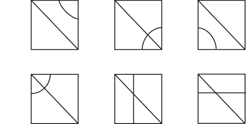
(a) $\lambda_{j}$ $\lambda_{i}$ $\lambda_{l}$ $\alpha$ (b) (c) (d) (e) (f) $\alpha$ $\alpha$ $\alpha$ $\alpha$ $\alpha$ $\lambda_{k}$ $\lambda_{m}$ $T_{1}$ $T_{2}$

Figure 3. Cases For Definition of Coordinate Change Maps

Consider an ideal triangulation $\lambda$ with edges $\lambda_{1}$, $\lambda_{2}$,…,$\lambda_{n}$, and let $\alpha$ be a simple closed curve in $S$ which is transverse to $\lambda$, where $\alpha$ does not backtrack over the edges of $\lambda$. Namely, $\alpha$ never enters a triangle of $S-\lambda$ through one side and exits through the same side.

Now consider a square $Q$ in the triangulation $\lambda$ formed by the edges $\lambda_{i}$, $\lambda_{j}$, $\lambda_{k}$, $\lambda_{l},$ and $\lambda_{m}$ as in Figure  3 (a). Then $\alpha$ can cross the square $Q$ several times. There are six possibilities for doing so, which are depicted in Figure  3. To each time $\alpha$ crosses $Q$, we associate a ”block” $B\in\bigotimes_{i=1}^{m}\mathcal{T}_{T_{i}}^{q^{\frac{1}{4}}}$ defined as follows.

1. $B=q^{-\frac{1}{4}}Z_{j,1}^{-1}Z_{k,1}^{-1}$ when $\alpha$ crosses $Q$ is as in Figure  3 (a).

2. $B=q^{-\frac{1}{2}}Z_{k,1}^{-1}Z_{i}^{-1}\hat{Z}_{l,2}^{-1}$ when $\alpha$ crosses $Q$ is as in Figure  3 (b).

3. $B=q^{-\frac{1}{4}}Z_{l,2}^{-1}Z_{m,2}^{-1}$ when $\alpha$ crosses $Q$ is as in Figure  3 (c).

4. $B=q^{\frac{1}{2}}Z_{j,1}^{-1}Z_{i}^{-1}Z_{m,2}^{-1}$ when $\alpha$ crosses $Q$ is as in Figure  3 (d).

5. $B=Z_{j,1}^{-1}Z_{i}^{-1}Z_{l,2}^{-1}$ when $\alpha$ crosses $Q$ is as in Figure  3 (e).

6. $B=Z_{k,1}^{-1}Z_{i}^{-1}Z_{m,2}^{-1}$ when $\alpha$ crosses $Q$ is as in Figure  3 (f).

Note the Weyl ordering of the $q$ coefficent of the block $B$ in each case.

Lemma 14.

Let $B_{1},B_{2},...,B_{r}$ be blocks associated to a simple closed curve $\alpha$ in $S$ crossing squares $Q_{1},Q_{2},...Q_{r}$ as in Figure  3.

Then every $T\in\hat{\mathcal{T}}_{\lambda}^{q^{\frac{1}{4}}}(\alpha)$ can be written in a unique way as $T=q^{w}B_{1}B_{2}...B_{r}R$ with $R\in\hat{\mathcal{T}}_{\lambda}^{q}$, where $q^{w}$ is the Weyl ordering coefficient of the blocks $B_{i}$.

Proof.

Every element $T\in\hat{\mathcal{T}}_{\lambda}^{q^{\frac{1}{4}}}(\alpha)$ can be written as $T=Z_{i_{1}}^{-1}Z_{i_{2}}^{-1}...Z_{i_{h}}^{-1}R$ with $R\in\hat{\mathcal{T}}_{\lambda}^{q}$. The result follows from the fact that $B_{1}B_{2}...B_{r}=q^{b}Z_{i_{1}}^{-1}Z_{i_{2}}^{-1}...Z_{i_{h}}^{-1}$ for some power of $q$.

∎

We now want to generalize to the non-commutative context the coordinate change isomorphisms $\Phi_{\lambda\lambda^{\prime}}^{q}$ from [7], described in the previous section, by introducing appropriate linear maps $\Theta^{q}_{\hat{\lambda}\lambda}:\hat{\mathcal{T}}_{\lambda}^{q^{\frac{1}{4}}}(\alpha)\rightarrow\hat{\mathcal{T}}_{\hat{\lambda}}^{q^{\frac{1}{4}}}(\alpha)$ in the following way:

Definition 15.

Given a simple closed curve $\alpha$ in the surface $S$, and $\alpha$-odd ideal triangulations $\lambda$, $\hat{\lambda}$ separated by a single diagonal exchange, define $\Theta^{q}_{\hat{\lambda}\lambda}:\hat{\mathcal{T}}_{\lambda}^{q^{\frac{1}{4}}}(\alpha)\rightarrow\hat{\mathcal{T}}_{\hat{\lambda}}^{q^{\frac{1}{4}}}(\alpha)$ as follows:

If $T=q^{w}B_{1}B_{2}...B_{r}R$ as in Lemma  14, $\Theta^{q}_{\hat{\lambda}\lambda}(T)$ is obtained from $T$ by

1. Keeping the same coefficient $q^{w}$

2. Replacing $R$ with $\Phi_{\hat{\lambda}\lambda}(R)\in\hat{\mathcal{T}}_{\hat{\lambda}}^{q}$

3. Replacing $B_{i}=q^{-\frac{1}{4}}Z_{j,1}^{-1}Z_{k,1}^{-1}$ with $\hat{B}_{i}=q^{-\frac{1}{2}}\hat{Z}_{j,1}^{-1}\hat{Z}_{i}^{-1}\hat{Z}_{k,2}^{-1}$ when the block $B_{i}$
   is associated to the configuration of Figure  3 (a).

4. Replacing $B_{i}=q^{-\frac{1}{2}}Z_{k,1}^{-1}Z_{i}^{-1}Z_{l,2}^{-1}$ with $\hat{B}_{i}=q^{-\frac{1}{4}}\hat{Z}_{k,2}^{-1}\hat{Z}_{l,2}^{-1}$ when the block $B_{i}$
   is associated to the configuration of Figure  3 (b).

5. Replacing $B_{i}=q^{-\frac{1}{4}}Z_{l,2}^{-1}Z_{m,2}^{-1}$ with $\hat{B}_{i}=q^{-\frac{1}{2}}\hat{Z}_{l,2}^{-1}\hat{Z}_{i}^{-1}\hat{Z}_{m,1}^{-1}$ when the block $B_{i}$
   is associated to the configuration of Figure  3 (c).

6. Replacing $B_{i}=q^{\frac{1}{2}}Z_{j,1}^{-1}Z_{i}^{-1}Z_{m,2}^{-1}$ with $\hat{B}_{i}=q^{\frac{1}{4}}\hat{Z}_{j,1}^{-1}\hat{Z}_{m,1}^{-1}$ when the block $B_{i}$
   is associated to the configuration of Figure  3 (d).

7. Replacing $B_{i}=Z_{j,1}^{-1}Z_{i}^{-1}Z_{l,2}^{-1}$ with $\hat{B}_{i}=\hat{Z}_{j,1}^{-1}(\hat{Z}_{i}+\hat{Z}_{i}^{-1})^{-1}\hat{Z}_{l,2}^{-1}$ when the block $B_{i}$
   is associated to the configuration of Figure  3 (e).

8. Replacing $B_{i}=Z_{k,1}^{-1}Z_{i}^{-1}Z_{m,2}^{-1}$ with $\hat{B}_{i}=\hat{Z}_{k,2}^{-1}(\hat{Z}_{i}+\hat{Z}_{i}^{-1})\hat{Z}_{m,1}^{-1}$ when the block $B_{i}$
   is associated to the configuration of Figure  3 (f).

Remark: $\Theta_{\hat{\lambda}\lambda}^{q}$ is only a linear map, not an algebra homomorphism. Indeed, $\hat{\mathcal{T}}_{\lambda}^{q^{\frac{1}{4}}}(\alpha)$ is not even an algebra.

Lemma 16.

$\Theta^{q}_{\hat{\lambda}\lambda}(T)$ is $\alpha$-odd.

Proof.

The only case which requires some thought is that of blocks of type (7) and (8) from Definition  15. However, note that in type (7)

$$\hat{B}_{i}=\hat{Z}_{j,1}^{-1}(\hat{Z}_{i}+\hat{Z}_{i}^{-1})^{-1}\hat{Z}_{l,2}^{-1}=\hat{Z}_{j,1}^{-1}\hat{Z}_{i}^{-1}(1+\hat{Z}_{i}^{-2})^{-1}\hat{Z}_{l,2}^{-1}=\hat{Z}_{j,1}^{-1}\hat{Z}_{i}^{-1}\hat{Z}_{l,2}^{-1}(1+q^{-1}\hat{Z}_{i}^{-2})^{-1}$$

with type (8) working the same way. ∎

Lemma 17.

The map $\Theta^{q}_{\hat{\lambda}\lambda}:\hat{\mathcal{T}}_{\lambda}^{q^{\frac{1}{4}}}(\alpha)\rightarrow\hat{\mathcal{T}}_{\hat{\lambda}}^{q^{\frac{1}{4}}}(\alpha)$ is independent of the order of the blocks $B_{i}$.

Proof.

Note that, when two blocks $B_{1}$, $B_{2}$ are replaced by blocks $\hat{B}_{1}$ and $\hat{B}_{2}$, then $\hat{B}_{1}$ and $\hat{B}_{2}$ satisfy the same skew commutativity relation as $B_{1}$ and $B_{2}$. Namely, if $B_{1}B_{2}=q^{2b}B_{2}B_{1}$, then $\hat{B}_{1}\hat{B}_{2}=q^{2b}\hat{B}_{2}\hat{B}_{1}$.

This follows from a simple computation. For instance, if $B_{1}$ and $B_{2}$ are respectively of type (7) and (8) of Definition 15 then:

$$\begin{split}B_{1}B_{2}&=(Z_{j,1}^{-1}Z_{i}^{-1}Z_{l,2}^{-1})(Z_{k,1}^{-1}Z_{i}^{-1}Z_{m,2}^{-1})\\ &=q^{-1}(Z_{k,1}^{-1}Z_{i}^{-1}Z_{m,2}^{-1})(Z_{j,1}^{-1}Z_{i}^{-1}Z_{l,2}^{-1})=q^{-1}B_{2}B_{1}\end{split}$$

and

$$\begin{split}\hat{B}_{1}\hat{B}_{2}&=(\hat{Z}_{j,1}^{-1}(\hat{Z}_{i}+\hat{Z}_{i}^{-1})^{-1}\hat{Z}_{l,2}^{-1})(\hat{Z}_{k,2}^{-1}(\hat{Z}_{i}+\hat{Z}_{i}^{-1})\hat{Z}_{m,1}^{-1})\\ &=(\hat{Z}_{j,1}^{-1}\hat{Z}_{l,2}^{-1})(\hat{Z}_{k,2}^{-1}(\hat{Z}_{i}+\hat{Z}_{i}^{-1})^{-1}(\hat{Z}_{i}+\hat{Z}_{i}^{-1})\hat{Z}_{m,1}^{-1})\\ &=(\hat{Z}_{j,1}^{-1}\hat{Z}_{l,2}^{-1})(\hat{Z}_{k,2}^{-1}\hat{Z}_{m,1}^{-1})=q^{-1}(\hat{Z}_{k,2}^{-1}\hat{Z}_{m,1}^{-1})(\hat{Z}_{j,1}^{-1}\hat{Z}_{l,2}^{-1})\\ &=q^{-1}(\hat{Z}_{k,2}^{-1}\hat{Z}_{m,1}^{-1})(\hat{Z}_{j,1}^{-1}(\hat{Z}_{i}+\hat{Z}_{i}^{-1})(\hat{Z}_{i}+\hat{Z}_{i}^{-1})^{-1}\hat{Z}_{l,2}^{-1})\\ &=q^{-1}(\hat{Z}_{k,2}^{-1}(\hat{Z}_{i}+\hat{Z}_{i}^{-1})\hat{Z}_{m,1}^{-1})(\hat{Z}_{j,1}^{-1}(\hat{Z}_{i}+\hat{Z}_{i}^{-1})^{-1}\hat{Z}_{l,2}^{-1})=q^{-1}\hat{B}_{2}\hat{B}_{1}.\end{split}$$

The result immediately follows from this property. ∎

The map $\Theta^{q}_{\hat{\lambda}\lambda}$ is specially designed so that:

Lemma 18.

For all $Z_{i_{1}}^{-1}Z_{i_{2}}^{-1}...Z_{i_{l}}^{-1}R\in\hat{\mathcal{T}}_{\lambda}^{q^{\frac{1}{4}}}(\alpha)$,

$[\Theta^{q}_{\hat{\lambda}\lambda}(Z_{i_{1}}^{-1}Z_{i_{2}}^{-1}...Z_{i_{l}}^{-1}R)]^{2}=\Phi_{\hat{\lambda}\lambda}((Z_{i_{1}}^{-1}Z_{i_{2}}^{-1}...Z_{i_{l}}^{-1}R)^{2})$, where $(Z_{i_{1}}^{-1}Z_{i_{2}}^{-1}...Z_{i_{l}}^{-1}R)^{2}\in\hat{\mathcal{T}}_{\lambda}^{q}$.

Proof.

This lemma follows from simple calculations. Given a simple closed curve $\alpha$ which crosses edges $\lambda_{i_{1}},...,\lambda_{i_{l}}$, label $Z_{\lambda}=Z_{i_{1}}^{-1}...Z_{i_{l}}^{-1}$. The definition of $\Theta^{q}_{\hat{\lambda}\lambda}$ was specifically designed so that

(1) $$\Phi_{\hat{\lambda}\lambda}((Z_{\lambda})^{2})=[\Theta^{q}_{\hat{\lambda}\lambda}(Z_{\lambda})]^{2}.$$

For example, consider $Z_{\lambda}=Z_{j,1}^{-1}Z_{i}^{-1}Z_{l,2}^{-1}$ as in (7) from Definition  15. Then we have:

$$\begin{split}[\Theta^{q}_{\hat{\lambda}\lambda}(Z_{\lambda})]^{2}&=[\Theta^{q}_{\hat{\lambda}\lambda}(Z_{j,1}^{-1}Z_{i}^{-1}Z_{l,2}^{-1})]^{2}\\ &=(\hat{Z}_{j,1}^{-1}(\hat{Z}_{i}+\hat{Z}_{i}^{-1})^{-1}\hat{Z}_{l,2}^{-1})(\hat{Z}_{j,1}^{-1}(\hat{Z}_{i}+\hat{Z}_{i}^{-1})^{-1}\hat{Z}_{l,2}^{-1})\\ &=(\hat{Z}_{j,1}^{-1}(1+\hat{Z}_{i}^{2})^{-1}\hat{Z}_{i}\hat{Z}_{l,2}^{-1})(\hat{Z}_{j,1}^{-1}\hat{Z}_{i}(1+\hat{Z}_{i}^{2})^{-1}\hat{Z}_{l,2}^{-1})\\ &=\hat{Z}_{j,1}^{-2}(1+q\hat{Z}_{i}^{2})^{-1}\hat{Z}_{i}^{2}(1+q^{-1}\hat{Z}_{i}^{2})^{-1}\hat{Z}_{l,2}^{-2}\\ &=\hat{Z}_{j,1}^{-2}(1+q\hat{Z}_{i}^{2})^{-1}\hat{Z}_{i}^{2}\hat{Z}_{l,2}^{-2}(1+q\hat{Z}_{i}^{2})^{-1}\\ &=\Phi_{\hat{\lambda}\lambda}(Z_{j,1}^{-2}Z_{i}^{-2}Z_{l,2}^{-2})=\Phi_{\hat{\lambda}\lambda}([Z_{j,1}^{-1}Z_{i}^{-1}Z_{l,2}^{-1}]^{2})\end{split}$$

Next we will prove a small lemma:

Sublemma 19.

Given a simple closed curve $\alpha$ which crosses edges $\lambda_{i_{1}},...,\lambda_{i,n}$ of ideal triangulation $\lambda$, then $\Phi_{\hat{\lambda}\lambda}(Z_{\lambda}X_{r}Z_{\lambda})=\Theta^{q}_{\hat{\lambda}\lambda}(Z_{\lambda})\Phi_{\hat{\lambda}\lambda}(X_{r})\Theta^{q}_{\hat{\lambda}\lambda}(Z_{\lambda})$ , for $Z_{\lambda}=Z_{i_{1}}^{-1}...Z_{i_{l}}^{-1}$ and for all $r\in\{1,2...n\}$.

Proof.

Given that $X_{r}Z_{\lambda}=q^{a}Z_{\lambda}X_{r}$ we have:

$$\begin{split}\Phi_{\hat{\lambda}\lambda}(Z_{\lambda}X_{r}Z_{\lambda})&=q^{a}\Phi_{\hat{\lambda}\lambda}(Z_{\lambda}Z_{\lambda}X_{r})=q^{a}\Phi_{\hat{\lambda}\lambda}(Z_{\lambda}Z_{\lambda})\Phi_{\hat{\lambda}\lambda}(X_{r})\\ &=q^{a}\Theta^{q}_{\hat{\lambda}\lambda}(Z_{\lambda})\Theta^{q}_{\hat{\lambda}\lambda}(Z_{\lambda})\Phi_{\hat{\lambda}\lambda}(X_{r})=\Theta^{q}_{\hat{\lambda}\lambda}(Z_{\lambda})\Phi_{\hat{\lambda}\lambda}(X_{r})\Theta^{q}_{\hat{\lambda}\lambda}(Z_{\lambda})\end{split}$$

∎

A direct corollary of Sublemma 19 is, given a polynomial $P\in\mathcal{T}_{\lambda}^{q}$, $\Phi_{\hat{\lambda}\lambda}(Z_{\lambda}PZ_{\lambda})=\Theta^{q}_{\hat{\lambda}\lambda}(Z_{\lambda})\Phi_{\hat{\lambda}\lambda}(P)\Theta^{q}_{\hat{\lambda}\lambda}(Z_{\lambda})$. Using this corollary, we then have, given polynomials $P,Q\in\mathcal{T}_{\lambda}^{q}$:

$$\begin{split}\Phi_{\hat{\lambda}\lambda}(Z_{\lambda}PQ^{-1}Z_{\lambda})&=\Phi_{\hat{\lambda}\lambda}(Z_{\lambda}PZ_{\lambda})\Phi_{\hat{\lambda}\lambda}(Z_{\lambda}^{-1}Q^{-1}Z_{\lambda})=\Theta^{q}_{\hat{\lambda}\lambda}(Z_{\lambda})\Phi_{\hat{\lambda}\lambda}(P)\Theta^{q}_{\hat{\lambda}\lambda}(Z_{\lambda})[\Phi_{\hat{\lambda}\lambda}(Z_{\lambda}QZ_{\lambda})]^{-1}\Phi_{\hat{\lambda}\lambda}(Z_{\lambda}^{2})\\ &=\Theta^{q}_{\hat{\lambda}\lambda}(Z_{\lambda})\Phi_{\hat{\lambda}\lambda}(P)\Theta^{q}_{\hat{\lambda}\lambda}(Z_{\lambda})[\Theta^{q}_{\hat{\lambda}\lambda}(Z_{\lambda})]^{-1}[\Phi_{\hat{\lambda}\lambda}(Q)]^{-1}[\Theta^{q}_{\hat{\lambda}\lambda}(Z_{\lambda})]^{-1}\Theta^{q}_{\hat{\lambda}\lambda}(Z_{\lambda})\Theta^{q}_{\hat{\lambda}\lambda}(Z_{\lambda})\text{ }(\text{Using }~{}\ref{Equ:SmallEquation})\\ &=\Theta^{q}_{\hat{\lambda}\lambda}(Z_{\lambda})\Phi_{\hat{\lambda}\lambda}(P)[\Phi_{\hat{\lambda}\lambda}(Q)]^{-1}\Theta^{q}_{\hat{\lambda}\lambda}(Z_{\lambda})=\Theta^{q}_{\hat{\lambda}\lambda}(Z_{\lambda})\Phi_{\hat{\lambda}\lambda}(PQ^{-1})\Theta^{q}_{\hat{\lambda}\lambda}(Z_{\lambda}).\end{split}$$

Now we can finally prove the lemma with the following computations:

$$\begin{split}&[\Theta^{q}_{\hat{\lambda}\lambda}(Z_{i_{1}}^{-1}Z_{i_{2}}^{-1}...Z_{i_{l}}^{-1}R)]^{2}=\Theta^{q}_{\hat{\lambda}\lambda}(Z_{i_{1}}^{-1}Z_{i_{2}}^{-1}...Z_{i_{l}}^{-1}R)\Theta^{q}_{\hat{\lambda}\lambda}(Z_{i_{1}}^{-1}Z_{i_{2}}^{-1}...Z_{i_{l}}^{-1}R)\\ &=\Theta^{q}_{\hat{\lambda}\lambda}(Z_{i_{1}}^{-1}Z_{i_{2}}^{-1}...Z_{i_{l}}^{-1})\Phi_{\hat{\lambda}\lambda}(R)\Theta^{q}_{\hat{\lambda}\lambda}(Z_{i_{1}}^{-1}Z_{i_{2}}^{-1}...Z_{i_{l}}^{-1})\Phi_{\hat{\lambda}\lambda}(R)\\ &=\Phi_{\hat{\lambda}\lambda}(Z_{i_{1}}^{-1}Z_{i_{2}}^{-1}...Z_{i_{l}}^{-1}RZ_{i_{1}}^{-1}Z_{i_{2}}^{-1}...Z_{i_{l}}^{-1})\Phi_{\hat{\lambda}\lambda}(R)\\ &=\Phi_{\hat{\lambda}\lambda}(Z_{i_{1}}^{-1}Z_{i_{2}}^{-1}...Z_{i_{l}}^{-1}RZ_{i_{1}}^{-1}Z_{i_{2}}^{-1}...Z_{i_{l}}^{-1}R)=\Phi_{\hat{\lambda}\lambda}([Z_{i_{1}}^{-1}Z_{i_{2}}^{-1}...Z_{i_{l}}^{-1}R]^{2})\end{split}$$

This concludes the proof of Lemma 18

∎

This leads us to another lemma.

Lemma 20.

If ideal triangulations $\lambda$ and $\hat{\lambda}$ are separated by a single diagonal exchange then the maps $\Theta^{q}_{\lambda\hat{\lambda}}$ and $\Theta^{q}_{\hat{\lambda}\lambda}$ are such that $\Theta^{q}_{\hat{\lambda}\lambda}=(\Theta^{q}_{\lambda\hat{\lambda}})^{-1}$

Proof.

To prove this it is sufficient to show this is true for the six blocks in Definition 15. Let the edges of $\lambda$ and $\hat{\lambda}$ involved in the diagonal exchange be labeled as represented in Figure 4. The result then follows from computations, all similar to the following.

$$\begin{split}(\Theta^{q}_{\lambda\hat{\lambda}})^{-1}(Z_{k,2}^{-1}(Z_{i}+Z_{i}^{-1})Z_{m,1}^{-1})&=\hat{Z}_{k,1}^{-1}\hat{Z}_{i}^{-1}\hat{Z}_{m,2}^{-1}\\ \Theta^{q}_{\hat{\lambda}\lambda}(Z_{k,2}^{-1}(Z_{i}+Z_{i}^{-1})Z_{m,1}^{-1})&=\Theta^{q}_{\hat{\lambda}\lambda}(Z_{k,2}^{-1}Z_{i}^{-1}(1+Z_{i}^{2})Z_{m,1}^{-1})\\ &=\Theta^{q}_{\hat{\lambda}\lambda}(Z_{k,2}^{-1}Z_{i}^{-1}Z_{m,1}^{-1}(1+q^{-1}Z_{i}^{2}))=\Theta^{q}_{\hat{\lambda}\lambda}(Z_{k,2}^{-1}Z_{i}^{-1}Z_{m,1}^{-1})\Phi_{\hat{\lambda}\lambda}((1+q^{-1}Z_{i}^{2}))\\ &=\hat{Z}_{k,1}^{-1}(\hat{Z}_{i}+\hat{Z}_{i}^{-1})^{-1}\hat{Z}_{m,2}^{-1}(1+q^{-1}\hat{Z}_{i}^{-2})=\hat{Z}_{k,1}^{-1}\hat{Z}_{i}^{-1}(1+\hat{Z}_{i}^{-2})^{-1}\hat{Z}_{m,2}^{-1}(1+q^{-1}\hat{Z}_{i}^{-2})\\ &=\hat{Z}_{k,1}^{-1}\hat{Z}_{i}^{-1}(1+\hat{Z}_{i}^{-2})^{-1}(1+\hat{Z}_{i}^{-2})\hat{Z}_{m,2}^{-1}=\hat{Z}_{k,1}^{-1}\hat{Z}_{i}^{-1}\hat{Z}_{m,2}^{-1}\end{split}$$

∎

$\lambda_{j}$ $\hat{\lambda}_{j}$ $\lambda_{l}$ $\hat{\lambda}_{l}$ $\lambda_{i}$ $\hat{\lambda}_{i}$ $\lambda_{m}$ $\hat{\lambda}_{k}$ $\lambda_{k}$ $\hat{\lambda}_{m}$ $T_{1}$ $T_{2}$ $T_{1}$ $T_{2}$

Figure 4. Diagonal Exchange

The following lemma about the $\Theta^{q}_{\lambda\hat{\lambda}}$ makes computations easier.

Lemma 21.

Given two ideal triangulations $\lambda$ and $\hat{\lambda}$ which differ only by a diagonal exchange and if the edges of $\lambda$ and $\hat{\lambda}$ involved in the diagonal exchange are labeled as depicted in Figure 4, then the following relations are satisfied:

$$\begin{split}\Theta^{q}_{\lambda\hat{\lambda}}(\hat{Z}_{j,1}\hat{Z}_{i}\hat{Z}_{l,2}+\hat{Z}_{j,1}^{-1}\hat{Z}_{i}\hat{Z}_{l,2}^{-1}+\hat{Z}_{j,1}^{-1}\hat{Z}_{i}^{-1}\hat{Z}_{l,2}^{-1})&=Z_{j,1}Z_{i}Z_{l,2}+Z_{j,1}Z_{i}^{-1}Z_{l,2}+Z_{j,1}^{-1}Z_{i}^{-1}Z_{l,2}^{-1}\\ \Theta^{q}_{\lambda\hat{\lambda}}(\hat{Z}_{k,1}\hat{Z}_{i}\hat{Z}_{m,2}+\hat{Z}_{k,1}\hat{Z}_{i}^{-1}\hat{Z}_{m,2}+\hat{Z}_{k,1}^{-1}\hat{Z}_{i}^{-1}\hat{Z}_{m,2}^{-1})&=Z_{k,1}Z_{i}Z_{m,2}+Z_{k,1}^{-1}Z_{i}Z_{m,2}^{-1}+Z_{k,1}^{-1}Z_{i}^{-1}Z_{m,2}^{-1}\\ \Theta^{q}_{\lambda\hat{\lambda}}(q^{-\frac{1}{4}}\hat{Z}_{j,1}\hat{Z}_{k,1}+q^{-\frac{1}{4}}\hat{Z}_{j,1}^{-1}\hat{Z}_{k,1}^{-1})&=q^{-\frac{1}{2}}Z_{j,1}Z_{i}Z_{k,1}+q^{-\frac{1}{2}}Z_{j,1}^{-1}Z_{i}^{-1}Z_{k,1}^{-1}\\ \Theta^{q}_{\lambda\hat{\lambda}}(q^{-\frac{1}{2}}\hat{Z}_{k,1}\hat{Z}_{i}\hat{Z}_{l,2}+q^{-\frac{1}{2}}\hat{Z}_{k,1}^{-1}\hat{Z}_{i}^{-1}\hat{Z}_{l,2}^{-1})&=q^{-\frac{1}{4}}Z_{k,2}Z_{l,2}+q^{-\frac{1}{4}}Z_{k,2}^{-1}Z_{l,2}^{-1}\\ \Theta^{q}_{\lambda\hat{\lambda}}(q^{\frac{1}{2}}\hat{Z}_{j,1}\hat{Z}_{i}\hat{Z}_{m,2}+q^{\frac{1}{2}}\hat{Z}_{j,1}^{-1}\hat{Z}_{i}^{-1}\hat{Z}_{m,2}^{-1})&=q^{\frac{1}{4}}Z_{j,1}Z_{m,1}+q^{\frac{1}{4}}Z_{j,1}^{-1}Z_{m,1}^{-1}\\ \Theta^{q}_{\lambda\hat{\lambda}}(q^{-\frac{1}{4}}\hat{Z}_{l,2}\hat{Z}_{m,2}+q^{-\frac{1}{4}}\hat{Z}_{l,2}^{-1}\hat{Z}_{m,2}^{-1})&=q^{-\frac{1}{2}}Z_{l,2}Z_{i}Z_{m,1}+q^{-\frac{1}{2}}Z_{l,1}^{-1}Z_{i}^{-1}Z_{m,2}^{-1}\\ \end{split}$$

Proof.

This lemma follows from simple calculations of which we will only do one.

The first line from the lemma is the result of the following computations:

$$\begin{split}&\Theta^{q}_{\lambda\hat{\lambda}}(\hat{Z}_{j,1}\hat{Z}_{i}\hat{Z}_{l,2}+\hat{Z}_{j,1}^{-1}\hat{Z}_{i}\hat{Z}_{l,2}^{-1}+\hat{Z}_{j,1}^{-1}\hat{Z}_{i}^{-1}\hat{Z}_{l,2}^{-1})\\ &=\Theta^{q}_{\lambda\hat{\lambda}}(q^{-1}\hat{Z}_{j,1}^{2}\hat{Z}_{j,1}^{-1}\hat{Z}_{i}^{-1}\hat{Z}_{l,2}^{-1}\hat{Z}_{i}^{2}\hat{Z}_{l,2}^{2}+q\hat{Z}_{i}^{2}\hat{Z}_{j,1}^{-1}\hat{Z}_{i}^{-1}\hat{Z}_{l,2}^{-1}+\hat{Z}_{j,1}^{-1}\hat{Z}_{i}^{-1}\hat{Z}_{l,2}^{-1})\\ &=q^{-1}(1+qZ_{i}^{2})Z_{j,1}^{2}Z_{j,1}^{-1}(Z_{i}+Z_{i}^{-1})^{-1}Z_{l,2}^{-1}Z_{i}^{-2}(1+qZ_{i}^{2})Z_{l,2}^{2}\\ &\qquad\qquad+qZ_{i}^{-2}Z_{j,1}^{-1}(Z_{i}+Z_{i}^{-1})^{-1}Z_{l,2}^{-1}+Z_{j,1}^{-1}(Z_{i}+Z_{i}^{-1})^{-1}Z_{l,2}^{-1}\\ &=q^{-1}Z_{j,1}(1+qZ_{i}^{2})(1+Z_{i}^{2})^{-1}Z_{i}Z_{l,2}^{-1}(Z_{i}^{-2}+q)Z_{l,2}^{2}+(1+qZ_{i}^{-2})Z_{j,1}^{-1}(Z_{i}+Z_{i}^{-1})^{-1}Z_{l,2}^{-1}\\ &=Z_{j,1}Z_{i}Z_{l,2}+q^{-1}Z_{j,1}Z_{i}Z_{l,2}^{-1}Z_{i}^{-2}Z_{l,2}^{2}+Z_{j,1}^{-1}(1+Z_{i}^{-2})(1+Z_{i}^{-2})^{-1}Z_{i}^{-1}Z_{l,2}^{-1}\\ &=Z_{j,1}Z_{i}Z_{l,2}+Z_{j,1}Z_{i}^{-1}Z_{l,2}+Z_{j,1}^{-1}Z_{i}^{-1}Z_{l,2}^{-1}\end{split}$$

∎

7. The Pentagon Relation for Square Roots

The goal of this section is to show that the linear maps $\Theta^{q}_{\lambda\hat{\lambda}}$ constructed in the previous section are compatible with the pentagon relation satisfied by the diagonal exchange maps, $\Delta_{i}$, which were introduced in Section 2.

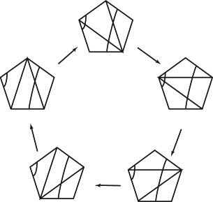
$\lambda_{a}$ $\lambda_{a}$ $\lambda_{a}$ $\lambda_{a}$ $\lambda_{b}$ $\lambda_{x}$ $\lambda_{y}$ $\lambda_{d}$ $\lambda_{e}$ $\lambda_{c}$ $\lambda^{2}$ $\lambda^{3}$ $\lambda^{4}$ $\lambda^{0}=\alpha_{x\rightarrow y}\lambda^{5}$ $\lambda^{1}$ $\alpha$ $\lambda_{a}$ $\beta$ $\lambda_{x}$ $\lambda_{y}$ $\lambda_{x}$ $\lambda_{y}$ $\lambda_{x}$ $\lambda_{y}$ $\lambda_{x}$ $\lambda_{y}$

Figure 5. The Pentagon Relation

Consider a pentagon cycle of geodesic laminations $\lambda^{0},\lambda^{1}=\Delta_{x}(\lambda^{0}),\lambda^{2}=\Delta_{y}(\lambda^{1}),\lambda^{3}=\Delta_{x}(\lambda^{2}),\lambda^{4}=\Delta_{y}(\lambda^{3}),\lambda^{5}=\Delta_{x}(\lambda^{4})=\alpha_{x\rightarrow y}(\lambda^{0})$ as represented in Figure  5.

Lemma 22.

The Pentagon Relation

$$\Theta^{q}_{\lambda^{0}\lambda^{1}}\circ\Theta^{q}_{\lambda^{1}\lambda^{2}}\circ\Theta^{q}_{\lambda^{2}\lambda^{3}}\circ\Theta^{q}_{\lambda^{3}\lambda^{4}}\circ\Theta^{q}_{\lambda^{4}\lambda^{5}}=\mathrm{Id}$$

is satisfied.

Proof.

There are only two non isotopic curves to consider, which are the $\alpha$ and $\beta$ curves depicted in Figure 5. First we will consider $\alpha$. If we let $\alpha$ be as represented in Figure 5 and label the edges of the pentagons also as depicted in Figure 5 then we really only need to look at where $q^{-\frac{1}{4}}Z_{d,1}^{-1}Z_{e,1}^{-1}$ is mapped to. If we apply the definition of $\Theta^{q}_{\lambda\hat{\lambda}}$ and use Lemma 20 on this monomial we obtain:

$$\begin{split}\Theta^{q}_{\lambda^{1}\lambda^{0}}(q^{-\frac{1}{4}}Z_{d,1}^{-1}Z_{e,1}^{-1})&=q^{-\frac{1}{2}}Z_{b,2}^{-1}Z_{x}^{-1}Z_{c,1}^{-1}\\ \Theta^{q}_{\lambda^{2}\lambda^{1}}(q^{-\frac{1}{2}}Z_{b,2}^{-1}Z_{x}^{-1}Z_{c,1}^{-1})&=q^{-\frac{1}{4}}Z_{e,3}^{-1}Z_{y,3}^{-1}q^{-\frac{1}{2}}Z_{y,2}^{-1}Z_{x}^{-1}Z_{a,1}^{-1}\\ &=q^{-\frac{3}{4}}Z_{e,3}^{-1}Z_{y}^{-1}Z_{x}^{-1}Z_{a,1}^{-1}\\ \Theta^{q}_{\lambda^{4}\lambda^{0}}(q^{-\frac{1}{4}}Z_{d,1}^{-1}Z_{e,1}^{-1})&=q^{-\frac{1}{4}}Z_{a,1}^{-1}Z_{b,1}^{-1}\\ \Theta^{q}_{\lambda^{3}\lambda^{4}}(q^{-\frac{1}{4}}Z_{a,1}^{-1}Z_{b,1}^{-1})&=q^{-\frac{1}{2}}Z_{c,2}^{-1}Z_{y}^{-1}Z_{d,1}^{-1}\\ \Theta^{q}_{\lambda^{2}\lambda^{3}}(q^{-\frac{1}{2}}Z_{c,2}^{-1}Z_{y}^{-1}Z_{d,1}^{-1})&=q^{-\frac{1}{2}}Z_{e,3}^{-1}Z_{y}^{-1}Z_{x,2}^{-1}q^{-\frac{1}{4}}Z_{x,1}^{-1}Z_{a,1}^{-1}\\ &=q^{-\frac{3}{4}}Z_{e,3}^{-1}Z_{y}^{-1}Z_{x}^{-1}Z_{a,1}^{-1}\\ \end{split}$$

Thus

$$\Theta^{q}_{\lambda^{0}\lambda^{1}}\circ\Theta^{q}_{\lambda^{1}\lambda^{2}}\circ\Theta^{q}_{\lambda^{2}\lambda^{3}}\circ\Theta^{q}_{\lambda^{3}\lambda^{4}}\circ\Theta^{q}_{\lambda^{4}\lambda_{(5)}}(q^{-\frac{1}{4}}Z_{d,1}^{-1}Z_{e,1}^{-1})$$

$$=Id(q^{-\frac{1}{4}}Z_{d,1}^{-1}Z_{e,1}^{-1})$$

.

Now we will consider $\beta$. If we let $\beta$ be as depicted in Figure 5 and label the edges of the pentagons also as represented in Figure 5 then we really only need to look at where $Z_{a,3}^{-1}Z_{x}^{-1}Z_{c,2}^{-1}$ is mapped to. If we apply the definition of $\Theta^{q}_{\lambda\hat{\lambda}}$ and use Lemma 20 on this monomial we obtain:

$$\begin{split}\Theta^{q}_{\lambda^{4}\lambda^{0}}&(Z_{a,3}^{-1}Z_{x}^{-1}Z_{c,2}^{-1})=Z_{c,3}^{-1}(Z_{y}+Z_{y}^{-1})^{-1}Z_{e,2}^{-1}\\ \Theta^{q}_{\lambda^{3}\lambda^{4}}&(Z_{c,3}^{-1}(Z_{y}+Z_{y}^{-1})^{-1}Z_{e,2}^{-1})=\Theta^{q}_{\lambda^{3}\lambda^{4}}(q^{-\frac{1}{4}}Z_{c,3}^{-1}z_{y,3}^{-1}q^{\frac{1}{4}}z_{y,2}^{-1}(1+Z_{y}^{-2})^{-1}Z_{e,2}^{-1})\\ &=q^{-\frac{1}{4}}Z_{e,1}^{-1}Z_{y}^{-1}Z_{x}^{-1}(1+Z_{x}^{-2}(1+qZ_{y}^{-2}))^{-1}Z_{b,3}^{-1}\\ \Theta^{q}_{\lambda^{1}\lambda^{0}}&(Z_{a,3}^{-1}Z_{x}^{-1}Z_{c,2}^{-1})=\Theta^{q}_{\lambda^{1}\lambda^{0}}(q^{\frac{1}{4}}Z_{a,3}^{-1}Z_{x,3}^{-1}q^{-\frac{1}{4}}Z_{x,2}^{-1}Z_{c,2}^{-1})\\ &=q^{-\frac{1}{4}}Z_{d,3}^{-1}Z_{y}^{-1}Z_{x}^{-1}Z_{a,1}^{-1}\\ \Theta^{q}_{\lambda^{2}\lambda^{1}}&(q^{-\frac{1}{4}}Z_{d,3}^{-1}Z_{y}^{-1}Z_{x}^{-1}Z_{a,1}^{-1})=\Theta^{q}_{\lambda^{2}\lambda^{1}}(q^{-\frac{1}{4}}Z_{d,3}^{-1}Z_{y}^{-1}Z_{x,2}^{-1}Z_{x,1}^{-1}Z_{a,1}^{-1})\\ &=q^{-\frac{1}{4}}Z_{b,1}^{-1}(Z_{x}+Z_{x}^{-1})^{-1}Z_{y}^{-1}Z_{d,2}^{-1}\\ \Theta^{q}_{\lambda^{3}\lambda^{2}}&(q^{-\frac{1}{4}}Z_{b,1}^{-1}(Z_{x}+Z_{x}^{-1})^{-1}Z_{y}^{-1}Z_{d,2}^{-1})\\ &=\Theta^{q}_{\lambda^{3}\lambda^{2}}(q^{-\frac{1}{4}}Z_{b,1}^{-1}(1+Z_{x}^{-2})^{-1}Z_{x,1}^{-1}Z_{x,3}^{-1}Z_{y}^{-1}Z_{d,2}^{-1})\\ &=q^{-\frac{1}{4}}Z_{e,1}^{-1}(1+Z_{y}^{-2}(1+qZ_{x}^{2})^{-1})^{-1}Z_{y}^{-1}(Z_{x}+Z_{x}^{-1})^{-1}Z_{b,3}^{-1}\\ &=q^{-\frac{1}{4}}Z_{e,1}^{-1}(1+q^{-1}Z_{x}^{2}Z_{y}^{-2})^{-1}Z_{y}^{-1}Z_{x}Z_{b,3}^{-1}\\ &=q^{-\frac{1}{4}}Z_{e,1}^{-1}(Z_{x}^{-2}+q^{-1}+Z_{x}^{-2}Z_{y}^{-2})^{-1}Z_{x}^{-2}Z_{y}^{-1}Z_{x}Z_{b,3}^{-1}\\ &=q^{-\frac{1}{4}}Z_{e,1}^{-1}Z_{y}^{-1}Z_{x}^{-1}(1+Z_{x}^{-2}(1+qZ_{y}^{-2}))^{-1}Z_{b,3}^{-1}\end{split}$$

Thus

$$\Theta^{q}_{\lambda^{0}\lambda^{1}}\circ\Theta^{q}_{\lambda^{1}\lambda^{2}}\circ\Theta^{q}_{\lambda^{2}\lambda^{3}}\circ\Theta^{q}_{\lambda^{3}\lambda^{4}}\circ\Theta^{q}_{\lambda^{4}\lambda^{5}}(Z_{a,3}^{-1}Z_{x}^{-1}Z_{c,2}^{-1})$$

$$=Id(Z_{a,3}^{-1}Z_{x}^{-1}Z_{c,2}^{-1})$$

.

∎

The diagonal exchanges and edge reindexings satisfy the following relations:

1. The Composition Relation: if $\delta$ and $\gamma$ are each either a diagonal exchange or a edge reindexing then $(\delta\gamma)(\lambda)=\delta\circ\gamma(\lambda)$.

2. The Reflexivity Relation: if $\Delta_{i}$ is an ith-diagonal exchange map then $\Delta_{i}^{2}(\lambda)=\lambda$.

3. The Reindexing Relation: If $\gamma\in S_{n}$ is a reindexing and $\Delta_{i}$ is an ith-diagonal exchange map then $\Delta_{i}\circ\gamma=\gamma\circ\Delta_{\gamma(i)}$.

4. The Distant Commutativity Relation: If $\lambda_{i}$ and $\lambda_{j}$ are edges of the ideal triangulation $\lambda\in\Lambda(S)$ that do not belong to the same triangle then $\Delta_{i}\circ\Delta_{j}(\lambda)=\Delta_{j}\circ\Delta_{i}(\lambda)$.

We now state the following two results of Penner. Refer to  [10] for their proofs.

Theorem 23.

Given two ideal triangulations $\lambda$, $\hat{\lambda}$, there exists a finite sequence of ideal triangulations $\lambda=\lambda^{0}$, $\lambda^{1}$, …,$\lambda^{m}=\hat{\lambda}$ such that $\lambda^{k+1}$ is obtained from $\lambda^{k}$ by a single diagonal exchange or by edge reindexing.

∎

Theorem 24.

Given two ideal triangulations $\lambda$, $\hat{\lambda}$ and two sequences of ideal triangulations $\lambda=\lambda^{0}$, $\lambda^{1}$, …,$\lambda^{m}=\hat{\lambda}$ and $\lambda=\hat{\lambda}^{0}$, $\hat{\lambda}^{1}$, …,$\hat{\lambda}^{m}=\hat{\lambda}$ such that $\lambda^{k+1}$ is obtained from $\lambda^{k}$ by a single diagonal exchange or by edge reindexing and $\hat{\lambda}^{k+1}$ is obtained from $\hat{\lambda}^{k}$ by a single diagonal exchange or by edge reindexing, these two sequences can be related to each other by applications of the following moves and their inverses:

1. Use the The Composition Relation to replace $...,\lambda^{k},\delta(\lambda^{k}),\gamma\circ\delta(\lambda^{k}),...$ with $...,\lambda^{k},(\gamma\delta)(\lambda^{k}),...$ where $\delta$ and $\gamma$ are each either a diagonal exchange or a edge reindexing.

2. Use The Reflexivity Relation to replace $...,\lambda^{k},...$ with $...,\lambda^{k},\Delta_{i}(\lambda^{k}),\lambda^{k}...$

3. Use The Reindexing Relation to replace $...,\lambda^{k},\gamma(\lambda^{k}),\Delta_{i}(\gamma(\lambda^{k})),...$ with $...,\lambda^{k},\Delta_{\gamma(i)}(\lambda^{k}),\gamma(\Delta_{\gamma(i)}(\lambda^{k})),...$ where $\gamma\in S_{n}$ is an edge reindexing.

4. Use The Distant Commutativity Relation to replace $...,\lambda^{k},...$ with $...,\lambda^{k},\Delta_{i}(\lambda^{k}),\Delta_{j}(\Delta_{i}(\lambda^{k})),\Delta_{j}(\lambda^{k}),\lambda^{k}...$ where $\lambda_{i}$ and $\lambda_{j}$ are two edges of $\lambda^{k}$ that do not belong to the same triangle.

5. Use The Pentagon Relation to replace $...,\lambda^{k},...$ with $...,\lambda^{k},\Delta_{i}(\lambda^{k}),\Delta_{j}\circ\Delta_{i}(\lambda^{k}),\Delta_{i}\circ\Delta_{j}\circ\Delta_{i}(\lambda^{k}),\Delta_{j}\circ\Delta_{i}\circ\Delta_{j}\circ\Delta_{i}(\lambda^{k}),\alpha_{i\leftrightarrow j}(\lambda^{k}),\lambda^{k},...$ where $\lambda_{i}$ and $\lambda_{j}$ are two diagonals of a pentagon of $\lambda^{k}$.

∎

Note: If we are given two ideal triangulations $\lambda$ and $\hat{\lambda}$ we can find a sequence of ideal triangulations $\lambda=\lambda^{0}$, $\lambda^{1}$, …,$\lambda^{m}=\hat{\lambda}$ where each $\lambda^{k+1}$ is obtained from $\lambda^{k}$ by a diagonal exchange or by an edge reindexing. Define $\Theta^{q}_{\lambda\hat{\lambda}}$, as the composition of the $\Theta^{q}_{\lambda^{k}\lambda^{k+1}}$. Lemma 20 and Lemma 22 along with Theorem  23 and Theorem  24 show that this $\Theta^{q}_{\lambda^{k}\lambda^{k+1}}$ is independent of the choice of the sequence of $\lambda^{k}$.

Theorem 25.

Given ideal triangulations $\lambda$, $\lambda^{\prime}$, $\lambda^{\prime\prime}$ then,

$$\Theta^{q}_{\lambda\lambda^{\prime\prime}}=\Theta^{q}_{\lambda\lambda^{\prime}}\circ\Theta^{q}_{\lambda^{\prime}\lambda^{\prime\prime}}$$

Proof.

This result simply follows from the definition.

∎

8. Punctured Tori

Figure 6. The Once Punctured Torus

Figure 7. A Torus With a Wide Hole and $p\geqslant 1$ Punctures

Let the once-punctured torus be the surface obtained by removing one point from a torus. Let a torus with a wide hole and $p\geqslant 1$ punctures be the surface that is obtained from the compact surface of genus one with one boundary component by removing $p\geqslant 1$ punctures from its boundary but none from its interior.

In this section, $S$ will denote either a once punctured torus or a torus with a wide hole and $p\geqslant 1$ punctures. Let $\Sigma(S)$ be the set of simple closed unoriented curves in $S$

Definition 26.

For an ideal triangulation $\lambda$ of $S$ with edges $\lambda_{1}$,…,$\lambda_{n}$ and given $\alpha\in\Sigma(S)$, define $\alpha$ as $\lambda$-simple if it meets each $\lambda_{i}$ in at most one point.

Definition 27.

Given an ideal triangulation $\lambda$ of $S$ with edges $\lambda_{1}$,…,$\lambda_{n}$ and given $\alpha\in\Sigma(S)$, define $\lambda$ as $\alpha$-simple if and only if $\alpha$ is $\lambda$-simple.

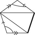
$\lambda_{j}$ $\lambda_{j}$ $\lambda_{k}$ $\lambda_{k}$ $\alpha$ $\alpha$ $T_{1}$ $T_{2}$

Figure 8. Two Dimensional Torus With a Wide Hole

We may now state the two main theorems of this section.

Theorem 28.

Let $S$ be either a once punctured torus or a torus with a wide hole and $p\geqslant 1$ punctures. There exists a family of $T_{\alpha}^{\lambda}\in\mathcal{T}_{\lambda}^{q^{\frac{1}{4}}}(\alpha)$, with $\lambda$ ranging over all ideal triangulations of $S$ and $\alpha$ over all essential simple closed curves of $S$, which satisfies:

1. If $\alpha$ is in $\Sigma(S)$ and $\lambda$ and $\hat{\lambda}$ are two triangulations of $S$, then $\Theta_{\lambda\hat{\lambda}}(T_{\alpha}^{\hat{\lambda}})=T_{\alpha}^{\lambda}$.

2. as $q\rightarrow 1$, $T_{\alpha}^{\lambda}$ converges to the non-quantum trace function $T_{\alpha}$ in $\mathcal{T}(S)$

3. If $\alpha$ and $\beta$ are disjoint, $T_{\alpha}^{\lambda}$ and $T_{\beta}^{\lambda}$ commute.

4. If $\alpha$ meets each edge of $\lambda$ at most once then $T_{\alpha}^{\lambda}$ is obtained from the classical trace $T_{\alpha}$ of Section 2.3 by multiplying each monomial by the Weyl ordering coefficient.

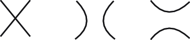
$\alpha$ $\beta$ $\alpha\beta$ $\beta\alpha$

Figure 9. Resolving Crossing in the Torus

Theorem 29.

The traces $T_{\alpha}^{\lambda}$ of Theorem 28 satisfy the following property: If $\alpha$ and $\beta$ meet in one point, and if $\alpha\beta$ and $\beta\alpha$ are obtained by resolving the intersection point as in Figure 9, then

$$T_{\alpha}^{\lambda}T_{\beta}^{\lambda}=qT_{\alpha\beta}^{\lambda}+q^{-1}T_{\beta\alpha}^{\lambda}.$$

In addition, $T_{\alpha}^{\lambda}$ with $\alpha$ non-separating is the only one which satisfy this property and conditions (1) and (4) of Theorem 28.

We restrict our attention to the case where $S$ is a torus with a wide hole and $p\geqslant 1$ punctures. The case of the once-punctured torus is similar, and simpler.

A key result used to prove Theorem 28 is the following proposition.

Proposition 30.

For an essential curve $\alpha$ in $\Sigma(S)$ and $\alpha$-simple ideal triangulations $\lambda$ and $\hat{\lambda}$ of $S$ there exists a sequence of ideal triangulations $\lambda=\lambda^{0}$ , $\lambda^{1}$ ,$\lambda^{2}$ ,…, $\lambda^{m-1}$ ,$\lambda^{m}=\hat{\lambda}$ such that each $\lambda^{i+1}$ is obtained from $\lambda^{i}$ by a diagonal exchange and $\lambda^{i}$ is $\alpha$-simple.

Proof.

To prove Proposition 30 we must prove the following lemmas.

Lemma 31.

If $\lambda$ and $\hat{\lambda}$ are $\alpha$-simple ideal triangulations of $S$, there exists a sequence of $\alpha$-simple ideal triangulations $\lambda=\lambda^{0}$ , $\lambda^{1}$ ,…, $\lambda^{m}$ and a sequence of $\alpha$-simple ideal triangulations $\hat{\lambda}=\hat{\lambda}^{0}$ , $\hat{\lambda}^{1}$ ,…, $\hat{\lambda}^{n}$ such that:

1. $\lambda^{l+1}$ is obtained from $\lambda^{l}$ by a diagonal exchange and $\hat{\lambda}^{l+1}$ is obtained from $\hat{\lambda}^{l}$ by a diagonal exchange

2. there exists edges $\lambda_{i}$ and $\hat{\lambda}_{j}$ of $\lambda^{m}$ and $\hat{\lambda}^{n}$, respectively, such that one component $C_{1}$ of $S-\lambda_{i}$ and one component $\hat{C}_{1}$ of $S-\hat{\lambda}_{j}$ are tori with exactly one spike at infinity.

3. $\lambda^{m}$ and $\hat{\lambda}^{n}$ coincide outside of $C_{1}$.

$S_{1}$ $S_{2}$ $S_{3}$ $S_{4}$ $S_{5}$

Figure 10. Quadrilateral in the Surface

Proof.

We will use the following proof for both $\lambda$ and $\hat{\lambda}$. Consider a quadrilateral as represented in Figure 10 with vertices at infinity $S_{1},S_{2},S_{3},S_{4}$, occurring counterclockwise in this order, and where and the edge from $S_{1}$ to $S_{2}$ is a boundary curve, the edges in this quadrilateral are edges $S_{1}$ to $S_{2}$, $S_{1}$ to $S_{3}$, $S_{1}$ to $S_{4}$, $S_{2}$ to $S_{3}$ and $S_{3}$ to $S_{4}$. If $S_{1}=S_{2}$ then we are done. Assume from now on that $S_{1}\neq S_{2}$

Case 1: If $S_{3}=S_{1}$ and $S_{4}=S_{1}$ then doing a diagonal exchange on both $\lambda$ and $\hat{\lambda}$ in this quadrilateral lowers the number of edges ending at $S_{1}$ by one. Also since $\alpha$ cannot cross the edge connecting $S_{1}$ to $S_{2}$ when you do this diagonal exchange the resulting triangulation remains $\alpha$-simple.

Case 2: If $S_{1}=S_{3}$ and $S_{1}\neq S_{4}$, then doing a diagonal exchange on both $\lambda$ and $\hat{\lambda}$ in this quadrilateral lowers the number of edges ending at $S_{1}$ by two. Also, the resulting triangulation remains $\alpha$-simple.

Case 3: If $S_{1}\neq S_{3}$ and $S_{1}\neq S_{4}$, then doing a diagonal exchange on both $\lambda$ and $\hat{\lambda}$ in this quadrilateral decreases the number of edges ending at $S_{1}$ by one. Also, the resulting triangulation remains $\alpha$-simple.

Case 4: If $S_{1}\neq S_{3}$ and $S_{1}=S_{4}$. then after doing a diagonal exchange on both $\lambda$ and $\hat{\lambda}$ in this quadrilateral if we consider the new quadrilateral created with edges $S_{1}$ to $S_{2}$, $S_{2}$ to $S_{4}$, $S_{1}$ to $S_{4}$ and a new point $S_{5}$ and edges $S_{1}$ to $S_{5}$ and $S_{4}$ to $S_{5}$ then we see that we are again in Case 2 or Case 3. Thus after another diagonal exchange on both $\lambda$ and $\hat{\lambda}$ in this new quadrilateral we reduce the number of edges ending at $S_{1}$ by one or two. For the same reason as above after the first diagonal exchange the resulting triangulation remains $\alpha$-simple and similarly after the second diagonal exchange the resulting triangulation remains $\alpha$-simple.

Now if we repeat this process until there are only two edges going to $S_{1}$ then we can effectively “forget” about the point at infinity $S_{1}$ and then repeat this process for another point at infinity. By the method of the proof we automatically get $\lambda^{m}$ and $\hat{\lambda}^{n}$ to coincide outside of $C_{1}$. ∎

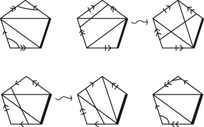
$T_{1}$ $T_{1}$ $\alpha$ $\alpha$ $\alpha$ $\alpha$ $\alpha$ $\alpha$ $\lambda_{i}$ $=$ $=$ $=$ $1$ $Diagonal$ $Exchange$ $2$ $Diagonal$ $Exchanges$

Figure 11. Pentagon Moves

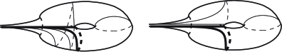
Figure 12. Torus Slope Changes

Lemma 32.

After changing the ideal triangulation $\lambda$ by $\alpha$-simple diagonal exchanges, we can arrange that, for the component $C_{1}$ of $S-\lambda_{i}$ which is a torus with one spike at infinity, the triangle $T_{1}$ containing $\partial C_{1}$ is disjoint from $\alpha$.

Proof.

This can be accomplished using moves similar to the ones represented in Figure 11.

∎

Change both triangulations $\lambda$ and $\hat{\lambda}$ such that the triangle $T_{1}$ containing $\partial C_{1}$ and $\partial\hat{C}_{1}$ is disjoint from $\alpha$ as in Lemma 32. If we consider the two nonboundary edges $\lambda_{1}$, $\lambda_{2}$ that make up the triangle $T_{1}$, they are completely determined by how many times they wrap around the boundary. Also, if edge $\lambda_{1}$ wraps around the boundary $k$ times then edge $\lambda_{2}$ is restricted to wrap around the boundary $k+1$ or $k-1$ times. Now it is clear from Figure 11 that if edges $\lambda_{1}$ and $\lambda_{2}$ wrap around the boundary $k$ and $k+1$ times respectively that through a series of $\alpha$-simple diagonal exchanges we can move to ideal triangulation $\lambda^{\prime}$ where the two edges $\lambda_{1}^{\prime}$ and $\lambda_{2}^{\prime}$, which are edges in the triangle on the boundary, wrap around the boundary either $k+1$ and $k+2$ time respectively or $k-1$ and $k$ times respectively. This is further illustrated in Figure 12. Thus we can change $\lambda$ and $\hat{\lambda}$ so that the edges $\lambda_{1}$ and $\lambda_{2}$ which make up the triangle on the boundary of $C_{1}$ and $\hat{C}_{1}$ coincide.

If we cut the surface along the edges $\lambda_{1}$ and $\lambda_{2}$ from above we are left with a cylinder with two spikes at infinity, four edges going between those spikes and $\alpha$ as a meridian of the cylinder as depicted in Figure 13. It is clear that, if we perform a diagonal exchange along any one of the two edges that spiral around the cylinder, the resulting ideal triangulation remains $\alpha$-simple. In addition, the diagonal exchanges of this type enable us to go between any two ideal triangulations of the cylinder.

Thus, we can always reduce an ideal triangulation to the case with only one spike at infinity.

This concludes the proof of Proposition  30 ∎

Figure 13. Cylinder in the Torus

We now prove Theorem 28 which we restate for the sake of the reader.

Theorem 33.

There exists a family of $T_{\alpha}^{\lambda}\in\mathcal{T}_{\lambda}^{q^{\frac{1}{4}}}(\alpha)$ with $\lambda$ ranging over all ideal triangulations of $S$ and $\alpha$ over all essential simple closed curves of $S$, which satisfies:

1. If $\alpha$ is in $\Sigma(S)$ and $\lambda$ and $\hat{\lambda}$ are two triangulations of $S$, then $\Theta_{\lambda\hat{\lambda}}(T_{\alpha}^{\hat{\lambda}})=T_{\alpha}^{\lambda}.$

2. as $q\rightarrow 1$, $T_{\alpha}^{\lambda}$ converges to the non-quantum trace function $T_{\alpha}$ in $\mathcal{T}(S).$

3. If $\alpha$ and $\beta$ are disjoint, $T_{\alpha}^{\lambda}$ and $T_{\beta}^{\lambda}$ commute.

4. If $\alpha$ meets each edge of $\lambda$ at most once then $T_{\alpha}^{\lambda}$ is obtained from the classical trace $T_{\alpha}$ of Section 2.3 by multiplying each monomial by the Weyl ordering coefficient.

Proof.

For an ideal triangulation $\lambda$ and a simple closed curve $\alpha$ in $S$ which is $\lambda$-simple, define $T_{\alpha}^{\lambda}$ to be obtained from the non-quantum trace function $T_{\alpha}$ by multiplying each monomial of $T_{\alpha}$ with the Weyl quantum ordering coefficient.

When $\alpha$ is not $\lambda$-simple and is not homotopic to the boundary, one easily finds an $\alpha$-simple ideal triangulation $\lambda^{*}$. In this case define $T_{\alpha}^{\lambda}=\Theta_{\lambda\lambda^{*}}(T_{\alpha}^{\lambda^{*}})$ where $T_{\alpha}^{\lambda^{*}}\in\hat{\mathcal{T}}_{\lambda^{*}}^{\frac{1}{4}}(\alpha)$ is defined by the previous case.

When $\alpha$ is not $\lambda$-simple and is homotopic to the boundary define $T_{\alpha}^{\lambda}$ to be obtained from the non-quantum trace function $T_{\alpha}$ by multiplying each monomial of $T_{\alpha}$ with the Weyl quantum ordering coefficient.

In the case where $\alpha$ is not homotopic to the boundary let us show that $T_{\alpha}^{\lambda}$ is well defined, namely is independent of the choice of the $\alpha$-simple ideal triangulation $\lambda^{*}$. The main step is to prove the following lemma.

Lemma 34.

For any two $\alpha$-simple ideal triangulations $\lambda,\hat{\lambda}$ of $S$, $\Theta_{\lambda\hat{\lambda}}(T_{\alpha}^{\hat{\lambda}})=T_{\alpha}^{\lambda}$.

Proof.

The main step in the proof is the following.

$\lambda_{j}$ $\hat{\lambda}_{j}$ $\lambda_{l}$ $\hat{\lambda}_{l}$ $\lambda_{i}$ $\hat{\lambda}_{i}$ $\lambda_{m}$ $\hat{\lambda}_{k}$ $\lambda_{k}$ $\hat{\lambda}_{m}$ $T_{1}$ $T_{2}$ $T_{1}$ $T_{2}$

Figure 14. Diagonal Exchange

Lemma 35.

Given two $\alpha$-simple ideal triangulations $\lambda$ and $\hat{\lambda}$ which differ by only one diagonal exchange, $\Theta_{\lambda\hat{\lambda}}(T_{\alpha}^{\hat{\lambda}})=T_{\alpha}^{\lambda}$.

Proof.

We must separate this into four cases, each represented in Figure 15. In each case we have $\alpha\in\Sigma(S)$ and $\alpha$-simple ideal triangulations $\lambda$ and $\hat{\lambda}$ with $\lambda$ and $\hat{\lambda}$ differing only by exchanging edge $\lambda_{i}$ and $\hat{\lambda}_{i}$. The edges of the quadrilaterals involved in the diagonal exchange are $\lambda_{i}$, $\lambda_{j}$, $\lambda_{k}$, $\lambda_{l}$, $\lambda_{m}$, $\hat{\lambda}_{i}$, $\hat{\lambda}_{j}$, $\hat{\lambda}_{k}$, $\hat{\lambda}_{l}$ and $\hat{\lambda}_{m}$ with the quadrilaterals edges in $\lambda$ and $\hat{\lambda}$ ordered as represented in Figure 14. This lemma follows from simple calculations of which we will do one of the four possible cases.

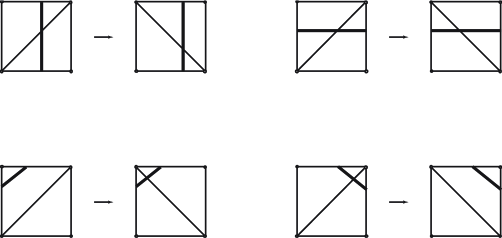
$\lambda_{j}$ $\hat{\lambda}_{j}$ $\lambda_{l}$ $\hat{\lambda}_{l}$ $\lambda_{i}$ $\hat{\lambda}_{i}$ $\lambda_{m}$ $\hat{\lambda}_{m}$ $\lambda_{k}$ $\hat{\lambda}_{k}$ $\alpha$ $\alpha$ Case 1 $\lambda_{j}$ $\hat{\lambda}_{j}$ $\lambda_{l}$ $\hat{\lambda}_{l}$ $\lambda_{i}$ $\hat{\lambda}_{i}$ $\lambda_{m}$ $\hat{\lambda}_{m}$ $\lambda_{k}$ $\hat{\lambda}_{k}$ $\alpha$ $\alpha$ Case 2 $\lambda_{j}$ $\hat{\lambda}_{j}$ $\lambda_{l}$ $\hat{\lambda}_{l}$ $\lambda_{i}$ $\hat{\lambda}_{i}$ $\lambda_{m}$ $\hat{\lambda}_{m}$ $\lambda_{k}$ $\hat{\lambda}_{k}$ $\alpha$ $\alpha$ Case 3 $\lambda_{j}$ $\hat{\lambda}_{j}$ $\lambda_{l}$ $\hat{\lambda}_{l}$ $\lambda_{i}$ $\hat{\lambda}_{i}$ $\lambda_{m}$ $\hat{\lambda}_{m}$ $\lambda_{k}$ $\hat{\lambda}_{k}$ $\alpha$ $\alpha$ Case 4

Figure 15.

Case 1: Let all edges of the quadrilateral be distinct and let the diagonal $\lambda_{i}$ go from the vertex adjoining $\hat{\lambda}_{j}$ to $\hat{\lambda}_{k}$ to the vertex adjoining $\hat{\lambda}_{l}$ to $\hat{\lambda}_{m}$. Also, let $\alpha$ cross edges $\hat{\lambda}_{j}$, $\hat{\lambda}_{i}$, and $\hat{\lambda}_{l}$ as depicted in Case 1 of Figure 15. Then by simple calculations we have:

$$\begin{split}T_{\alpha}^{\hat{\lambda}}=&\hat{A}(\hat{Z}_{j,2}\hat{Z}_{i}\hat{Z}_{l,1}+\hat{Z}_{j,2}^{-1}\hat{Z}_{i}\hat{Z}_{l,1}^{-1}+\hat{Z}_{j,2}^{-1}\hat{Z}_{i}^{-1}\hat{Z}_{l,1}^{-1})\hat{B}+\hat{C}(q^{-\frac{1}{2}}\hat{Z}_{j,2}\hat{Z}_{i}\hat{Z}_{l,1}^{-1})\hat{D}+\hat{E}(q^{\frac{1}{2}}\hat{Z}_{j,2}^{-1}\hat{Z}_{i}\hat{Z}_{l,1})\hat{F}\\ &\hat{A},\hat{B},\hat{C},\hat{D},\hat{E},\hat{F}\in\mathcal{T}_{\hat{\lambda}}^{q^{\frac{1}{4}}}\\ \end{split}$$

and

$$\begin{split}\Theta_{\lambda\hat{\lambda}}(T_{\alpha}^{\hat{\lambda}})&=\Theta_{\lambda\hat{\lambda}}(\hat{A}(\hat{Z}_{j,2}\hat{Z}_{i}\hat{Z}_{l,1}+\hat{Z}_{j,2}^{-1}\hat{Z}_{i}\hat{Z}_{l,1}^{-1}+\hat{Z}_{j,2}^{-1}\hat{Z}_{i}^{-1}\hat{Z}_{l,1}^{-1})\hat{B}+\hat{C}(q^{-\frac{1}{2}}\hat{Z}_{j,2}\hat{Z}_{i}\hat{Z}_{l,1}^{-1})\hat{D}+\hat{E}(q^{-\frac{1}{2}}\hat{Z}_{j,2}^{-1}\hat{Z}_{i}\hat{Z}_{l,1})\hat{F})\\ &=A(\Theta_{\lambda\hat{\lambda}}(\hat{Z}_{j,2}^{-1}\hat{Z}_{i}^{-1}\hat{Z}_{l,1}^{-1}\hat{Z}_{j,2}^{2}\hat{Z}_{i}^{2}\hat{Z}_{l,1}^{2}+q^{-1}\hat{Z}_{j,2}^{-1}\hat{Z}_{i}^{-1}\hat{Z}_{l,1}^{-1}\hat{Z}_{i}^{2}+\hat{Z}_{j,2}^{-1}\hat{Z}_{i}^{-1}\hat{Z}_{l,1}^{-1}))B\\ &\quad\quad\quad+C(\Theta_{\lambda\hat{\lambda}}(q^{\frac{1}{2}}\hat{Z}_{j,2}^{-1}\hat{Z}_{i}^{-1}\hat{Z}_{l,1}^{-1}\hat{Z}_{j,2}^{2}\hat{Z}_{i}^{2}))D+E(\Theta_{\lambda\hat{\lambda}}(q^{-\frac{3}{2}}\hat{Z}_{j,2}^{-1}\hat{Z}_{i}^{-1}\hat{Z}_{l,1}^{-1}\hat{Z}_{i}^{2}\hat{Z}_{l,1}^{2}))F\\ &=A(Z_{j,1}^{-1}(Z_{i}+Z_{i}^{-1})^{-1}Z_{l,2}^{-1}(1+qZ_{i}^{2})Z_{j,1}^{2}Z_{i}^{-2}(1+qZ_{i}^{2})Z_{l,2}^{2}\\ &\quad\quad\quad+q^{-1}Z_{j,1}^{-1}(Z_{i}+Z_{i}^{-1})^{-1}Z_{l,2}^{-1}Z_{i}^{-2}+Z_{j,1}^{-1}(Z_{i}+Z_{i}^{-1})^{-1}Z_{l,2}^{-1})B\\ &\quad\quad\quad+C(q^{\frac{1}{2}}Z_{j,1}^{-1}(Z_{i}+Z_{i}^{-1})^{-1}Z_{l,2}^{-1}(1+qZ_{i}^{2})Z_{j,1}^{2}Z_{i}^{-2})D\\ &\quad\quad\quad+E(q^{-\frac{3}{2}}Z_{j,1}^{-1}(Z_{i}+Z_{i}^{-1})^{-1}Z_{l,2}^{-1}Z_{i}^{-2}(1+qZ_{i}^{2})Z_{l,2}^{2})F\\ &=A(Z_{j,1}^{-1}Z_{i}(1+Z_{i}^{2})^{-1}(1+Z_{i}^{2})Z_{l,2}^{-1}Z_{j,1}^{2}Z_{i}^{-2}(1+qZ_{i}^{2})Z_{l,2}^{2}\\ &\quad\quad\quad+Z_{j,1}^{-1}(Z_{i}+Z_{i}^{-1})^{-1}Z_{i}^{-2}Z_{l,2}^{-1}+Z_{j,1}^{-1}(Z_{i}+Z_{i}^{-1})^{-1}Z_{l,2}^{-1})B\\ &\quad\quad\quad+C(q^{\frac{1}{2}}Z_{j,1}Z_{i}^{-1}Z_{l,2}^{-1})D+E(q^{-\frac{1}{2}}Z_{j,1}^{-1}Z_{i}^{-1}Z_{l,2})F\\ &=A(Z_{j,1}(Z_{i}^{-1}+Z_{i})Z_{l,2}+Z_{j,1}^{-1}Z_{i}^{-1}(1+Z_{i}^{-2})^{-1}(Z_{i}^{-2}+1)Z_{l,2}^{-1})B\\ &\quad\quad\quad+C(q^{\frac{1}{2}}Z_{j,1}Z_{i}^{-1}Z_{l,2}^{-1})D+E(q^{-\frac{1}{2}}Z_{j,1}^{-1}Z_{i}^{-1}Z_{l,2})F\\ &=A(Z_{j,1}Z_{i}Z_{l,2}+Z_{j,1}Z_{i}^{-1}Z_{l,2}+Z_{j,1}^{-1}Z_{i}^{-1}Z_{l,2}^{-1})B\\ &\quad\quad\quad+C(q^{\frac{1}{2}}Z_{j,1}Z_{i}^{-1}Z_{l,2}^{-1})D+E(q^{-\frac{1}{2}}Z_{j,1}^{-1}Z_{i}^{-1}Z_{l,2})F=T_{\alpha}^{\lambda}\\ &\quad\quad\quad\quad\quad\quad A,B,C,D,E,F\in\mathcal{T}_{\lambda}^{q^{\frac{1}{4}}}\\ \end{split}$$

∎

Lemma 34 is now a direct corollary of Proposition 30 and Lemma 35. ∎

Lemma 34 proves that the definition of $T_{\alpha}^{\lambda}$ is independent of the choice of triangulation $\lambda^{*}$.

Consider two triangulations $\lambda$ and $\hat{\lambda}$ and an essential simple closed curve $\alpha$. From the above definition we have that there exists an $\alpha$-simple ideal triangulation $\lambda^{*}$ such that $T_{\alpha}^{\lambda}=\Theta_{\lambda\lambda^{*}}(T_{\alpha}^{\lambda^{*}})$ and $T_{\alpha}^{\hat{\lambda}}=\Theta_{\hat{\lambda}\lambda^{*}}(T_{\alpha}^{\lambda^{*}})$. Thus $\Theta_{\lambda\lambda^{*}}^{-1}(T_{\alpha}^{\lambda})=\Theta_{\hat{\lambda}\lambda^{*}}^{-1}(T_{\alpha}^{\hat{\lambda}})$, which implies that $T_{\alpha}^{\lambda}=\Theta_{\lambda\lambda^{*}}(\Theta_{\hat{\lambda}\lambda^{*}}^{-1}(T_{\alpha}^{\hat{\lambda^{\prime}}}))$. Since we know that $\Theta_{\hat{\lambda}\lambda^{*}}^{-1}=\Theta_{\lambda^{*}\hat{\lambda}}$ and $\Theta_{\lambda\hat{\lambda}}=\Theta_{\lambda\lambda^{*}}\circ\Theta_{\lambda^{*}\hat{\lambda}}$ this implies that $T_{\alpha}^{\lambda}=\Theta_{\lambda\hat{\lambda}}(T_{\alpha}^{\hat{\lambda}})$. Thus property (1) of Theorem 33 holds.

Now we must show that if $\alpha$ is a simple closed curve in $S$ and is homotopic to the boundary, then $T_{\alpha}^{\lambda}$ also satisfies property (1) of Theorem 33. The main step is to prove the following lemma.

Lemma 36.

For any two ideal triangulations $\lambda,\hat{\lambda}$ of $S$, $\Theta_{\lambda\hat{\lambda}}(T_{\alpha}^{\hat{\lambda}})=T_{\alpha}^{\lambda}$.

Proof.

The main step in the proof is the following.

Lemma 37.

Given two ideal triangulations $\lambda$ and $\hat{\lambda}$ which differ by only one diagonal exchange, $\Theta_{\lambda\hat{\lambda}}(T_{\alpha}^{\hat{\lambda}})=T_{\alpha}^{\lambda}$.

Proof.

We must separate this into four cases, each of which are represented in Figure  16. In each case we have $\alpha\in\Sigma(S)$ homotopic to the boundary and $\lambda$ and $\hat{\lambda}$ differing only by exchanging edge $\lambda_{i}$ and $\hat{\lambda}_{i}$. The edges of the quadrilaterals involved in the diagonal exchange are $\lambda_{i}$, $\lambda_{j}$, $\lambda_{k}$, $\lambda_{l}$, $\lambda_{m}$, $\hat{\lambda}_{i}$, $\hat{\lambda}_{j}$, $\hat{\lambda}_{k}$, $\hat{\lambda}_{l}$ and $\hat{\lambda}_{m}$ with the quadrilaterals edges in $\lambda$ and $\hat{\lambda}$ ordered as represented in Figure 17. This lemma follows from simple calculations nearly identical to those in Lemma  35 which we omit for the sake of brevity.

∎

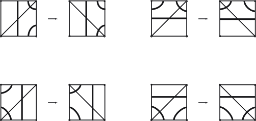
$\lambda_{j}$ $\hat{\lambda}_{j}$ $\lambda_{l}$ $\hat{\lambda}_{l}$ $\lambda_{i}$ $\hat{\lambda}_{i}$ $\lambda_{m}$ $\hat{\lambda}_{m}$ $\lambda_{k}$ $\hat{\lambda}_{k}$ $\alpha$ $\alpha$ Case 1 $\lambda_{j}$ $\hat{\lambda}_{j}$ $\lambda_{l}$ $\hat{\lambda}_{l}$ $\lambda_{i}$ $\hat{\lambda}_{i}$ $\lambda_{m}$ $\hat{\lambda}_{m}$ $\lambda_{k}$ $\hat{\lambda}_{k}$ $\alpha$ $\alpha$ Case 2 $\lambda_{j}$ $\hat{\lambda}_{j}$ $\lambda_{l}$ $\hat{\lambda}_{l}$ $\lambda_{i}$ $\hat{\lambda}_{i}$ $\lambda_{m}$ $\hat{\lambda}_{m}$ $\lambda_{k}$ $\hat{\lambda}_{k}$ $\alpha$ $\alpha$ Case 3 $\lambda_{j}$ $\hat{\lambda}_{j}$ $\lambda_{l}$ $\hat{\lambda}_{l}$ $\lambda_{i}$ $\hat{\lambda}_{i}$ $\lambda_{m}$ $\hat{\lambda}_{m}$ $\lambda_{k}$ $\hat{\lambda}_{k}$ $\alpha$ $\alpha$ Case 4

Figure 16.

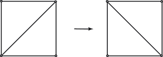
$\lambda_{j}$ $\hat{\lambda}_{j}$ $\lambda_{l}$ $\hat{\lambda}_{l}$ $\lambda_{i}$ $\hat{\lambda}_{i}$ $\lambda_{m}$ $\hat{\lambda}_{k}$ $\lambda_{k}$ $\hat{\lambda}_{m}$ $T_{1}$ $T_{2}$ $T_{1}$ $T_{2}$

Figure 17. Diagonal Exchange

Lemma 36 is now a direct corollary of Theorem 23 and Lemma 37. ∎

Properties (2) and (3) of Theorem 33 both follow from definitions. Property (4) of Theorem 33 follows from the way we defined the non-quantum traces and the fact that this definition is well-defined. This concludes the proof of Theorem 33 (Theorem 28). ∎

We now prove Theorem 29 which we restate for the sake of the reader.

Theorem 38.

The traces $T_{\alpha}^{\lambda}$ of Theorem 33 satisfy the following property: If $\alpha$ and $\beta$ meet in one point, and if $\alpha\beta$ and $\beta\alpha$ are obtained by resolving the intersection point as in Figure 18, then

$$T_{\alpha}^{\lambda}T_{\beta}^{\lambda}=q^{\frac{1}{2}}T_{\alpha\beta}^{\lambda}+q^{-\frac{1}{2}}T_{\beta\alpha}^{\lambda}.$$

In addition, $T_{\alpha}^{\lambda}$ with $\alpha$ non-separating is the only one which satisfy this property and conditions (1) and (4) of Theorem 33.

$\alpha$ $\beta$ $\alpha\beta$ $\beta\alpha$

Figure 18. Resolving Crossing in the Torus

Proof.

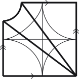
$\lambda_{j}$ $\lambda_{k}$ $\lambda_{i}$ $\lambda_{h}$ $\alpha$ $\beta$ $\alpha\beta$ $\alpha\beta$ $\beta\alpha$ $\beta\alpha$

Figure 19. Quadrilateral Labeling

Notice that Property (1) from Theorem 33 implies that it suffices to show $T_{\alpha}^{\lambda}T_{\beta}^{\lambda}=q^{\frac{1}{2}}T_{\alpha\beta}^{\lambda}+q^{-\frac{1}{2}}T_{\beta\alpha}^{\lambda}$ for one particular $\lambda$. So, we can choose $\lambda$ to be the ideal triangulation represented in Figure 19. In particular, $\alpha$, $\beta$ and $\alpha\beta$ are $\lambda$-simple and $\beta\alpha$ is not. From Theorem 33 $T_{\alpha}^{\lambda}$, $T_{\beta}^{\lambda}$, and $T_{\alpha\beta}^{\lambda}$ are uniquely determined and:

$$\begin{split}T_{\alpha}^{\lambda}&=q^{\frac{1}{4}}Z_{k,1}Z_{h}Z_{i}Z_{k,3}+q^{\frac{1}{4}}Z_{k,1}Z_{h}^{-1}Z_{i}Z_{k,3}+q^{\frac{1}{4}}Z_{k,1}Z_{h}^{-1}Z_{i}^{-1}Z_{k,3}+q^{\frac{1}{4}}Z_{k,1}^{-1}Z_{h}^{-1}Z_{i}^{-1}Z_{k,3}^{-1}\\ T_{\beta}^{\lambda}&=q^{\frac{1}{4}}Z_{j,1}Z_{h}Z_{i}Z_{j,3}+q^{\frac{1}{4}}Z_{j,1}^{-1}Z_{h}Z_{i}Z_{j,3}^{-1}+q^{\frac{1}{4}}Z_{j,1}^{-1}Z_{h}^{-1}Z_{i}Z_{j,3}^{-1}+q^{\frac{1}{4}}Z_{j,1}^{-1}Z_{h}^{-1}Z_{i}^{-1}Z_{j,3}^{-1}\\ T_{\alpha\beta}^{\lambda}&=Z_{k,1}Z_{h}^{-1}Z_{i}^{-1}Z_{k,3}Z_{j,1}Z_{h}Z_{i}Z_{j,3}+Z_{k,1}^{-1}Z_{h}^{-1}Z_{i}^{-1}Z_{k,3}^{-1}Z_{j,1}Z_{h}Z_{i}Z_{j,3}+Z_{k,1}^{-1}Z_{h}^{-1}Z_{i}^{-1}Z_{k,3}^{-1}Z_{j,1}^{-1}Z_{h}Z_{i}Z_{j,3}^{-1}\end{split}$$

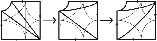
$\lambda_{i}$ $\lambda_{i}^{\prime}$ $\lambda_{i}^{\prime\prime}$ $\lambda_{h}$ $\lambda_{h}^{\prime}$ $\lambda_{h}^{\prime\prime}$

Figure 20. Diagonal Moves in the Torus

To find $T_{\beta\alpha}^{\lambda}$ we perform two diagonal exchanges, changing $\lambda$ to $\lambda^{\prime}$ and then $\lambda^{\prime\prime}$ respectively, as represented in Figure 20. Because $\beta\alpha$ is $\lambda^{\prime\prime}$-simple $T_{\beta\alpha}^{\lambda^{\prime\prime}}$ can be determined. To calculate $T_{\beta\alpha}^{\lambda}$ we simply use the coordinate change maps and set $T_{\beta\alpha}^{\lambda}=\Theta_{\lambda\lambda^{\prime\prime}}(T_{\beta\alpha}^{\lambda^{\prime\prime}})$. The computations use Lemma 21 four times, and yield:

$$\begin{split}T_{\beta\alpha}^{\lambda}&=\Theta_{\lambda\lambda^{\prime\prime}}(T_{\beta\alpha}^{\lambda^{\prime\prime}})=Z_{k,1}Z_{h}Z_{i}Z_{k,3}Z_{j,1}Z_{h}Z_{i}Z_{j,3}+Z_{k,1}Z_{h}Z_{i}Z_{k,3}Z_{j,1}^{-1}Z_{h}Z_{i}Z_{j,3}^{-1}\\ &+Z_{k,1}Z_{h}Z_{i}Z_{k,3}Z_{j,1}^{-1}Z_{h}^{-1}Z_{i}Z_{j,3}^{-1}+Z_{k,1}Z_{h}Z_{i}Z_{k,3}Z_{j,1}^{-1}Z_{h}^{-1}Z_{i}^{-1}Z_{j,3}^{-1}+Z_{k,1}Z_{h}^{-1}Z_{i}Z_{k,3}Z_{j,1}Z_{h}Z_{i}Z_{j,3}\\ &+Z_{k,1}Z_{h}^{-1}Z_{i}Z_{k,3}Z_{j,1}^{-1}Z_{h}Z_{i}Z_{j,3}^{-1}+Z_{k,1}Z_{h}^{-1}Z_{i}Z_{k,3}Z_{j,1}^{-1}Z_{h}^{-1}Z_{i}Z_{j,3}^{-1}+Z_{k,1}Z_{h}^{-1}Z_{i}Z_{k,3}Z_{j,1}^{-1}Z_{h}^{-1}Z_{i}^{-1}Z_{j,3}^{-1}\\ &+Z_{k,1}Z_{h}^{-1}Z_{i}^{-1}Z_{k,3}Z_{j,1}^{-1}Z_{h}Z_{i}Z_{j,3}^{-1}+Z_{k,1}Z_{h}^{-1}Z_{i}^{-1}Z_{k,3}Z_{j,1}^{-1}Z_{h}^{-1}Z_{i}Z_{j,3}^{-1}+Z_{k,1}Z_{h}^{-1}Z_{i}^{-1}Z_{k,3}Z_{j,1}^{-1}Z_{h}^{-1}Z_{i}^{-1}Z_{j,3}^{-1}\\ &+Z_{k,1}^{-1}Z_{h}^{-1}Z_{i}^{-1}Z_{k,3}^{-1}Z_{j,1}^{-1}Z_{h}^{-1}Z_{i}Z_{j,3}^{-1}+Z_{k,1}^{-1}Z_{h}^{-1}Z_{i}^{-1}Z_{k,3}^{-1}Z_{j,1}^{-1}Z_{h}^{-1}Z_{i}^{-1}Z_{j,3}^{-1}\end{split}$$

Finally we directly compute that $T_{\alpha}^{\lambda}T_{\beta}^{\lambda}=q^{\frac{1}{2}}T_{\alpha\beta}^{\lambda}+q^{-\frac{1}{2}}T_{\beta\alpha}^{\lambda}$ in the following way:

$$\begin{split}T_{\alpha}^{\lambda}T_{\beta}^{\lambda}&=q^{\frac{1}{2}}Z_{k,1}Z_{h}Z_{i}Z_{k,3}Z_{j,1}Z_{h}Z_{i}Z_{j,3}+q^{\frac{1}{2}}Z_{k,1}Z_{h}Z_{i}Z_{k,3}Z_{j,1}^{-1}Z_{h}Z_{i}Z_{j,3}^{-1}\\ &\qquad+q^{\frac{1}{2}}Z_{k,1}Z_{h}Z_{i}Z_{k,3}Z_{j,1}^{-1}Z_{h}^{-1}Z_{i}Z_{j,3}^{-1}+q^{\frac{1}{2}}Z_{k,1}Z_{h}Z_{i}Z_{k,3}Z_{j,1}^{-1}Z_{h}^{-1}Z_{i}^{-1}Z_{j,3}^{-1}\\ &\qquad+q^{\frac{1}{2}}Z_{k,1}Z_{h}^{-1}Z_{i}Z_{k,3}Z_{j,1}Z_{h}Z_{i}Z_{j,3}+q^{\frac{1}{2}}Z_{k,1}Z_{h}^{-1}Z_{i}Z_{k,3}Z_{j,1}^{-1}Z_{h}Z_{i}Z_{j,3}^{-1}\\ &\qquad+q^{\frac{1}{2}}Z_{k,1}Z_{h}^{-1}Z_{i}Z_{k,3}Z_{j,1}^{-1}Z_{h}^{-1}Z_{i}Z_{j,3}^{-1}+q^{\frac{1}{2}}Z_{k,1}Z_{h}^{-1}Z_{i}Z_{k,3}Z_{j,1}^{-1}Z_{h}^{-1}Z_{i}^{-1}Z_{j,3}^{-1}\\ &\qquad+q^{\frac{1}{2}}Z_{k,1}Z_{h}^{-1}Z_{i}^{-1}Z_{k,3}Z_{j,1}Z_{h}Z_{i}Z_{j,3}+q^{\frac{1}{2}}Z_{k,1}Z_{h}^{-1}Z_{i}^{-1}Z_{k,3}Z_{j,1}^{-1}Z_{h}Z_{i}Z_{j,3}^{-1}\\ &\qquad+q^{\frac{1}{2}}Z_{k,1}Z_{h}^{-1}Z_{i}^{-1}Z_{k,3}Z_{j,1}^{-1}Z_{h}^{-1}Z_{i}Z_{j,3}^{-1}+q^{\frac{1}{2}}Z_{k,1}Z_{h}^{-1}Z_{i}^{-1}Z_{k,3}Z_{j,1}^{-1}Z_{h}^{-1}Z_{i}^{-1}Z_{j,3}^{-1}\\ &\qquad+q^{\frac{1}{2}}Z_{k,1}^{-1}Z_{h}^{-1}Z_{i}^{-1}Z_{k,3}^{-1}Z_{j,1}Z_{h}Z_{i}Z_{j,3}+q^{\frac{1}{2}}Z_{k,1}^{-1}Z_{h}^{-1}Z_{i}^{-1}Z_{k,3}^{-1}Z_{j,1}^{-1}Z_{h}Z_{i}Z_{j,3}^{-1}\\ &\qquad+q^{\frac{1}{2}}Z_{k,1}^{-1}Z_{h}^{-1}Z_{i}^{-1}Z_{k,3}^{-1}Z_{j,1}^{-1}Z_{h}^{-1}Z_{i}Z_{j,3}^{-1}+q^{\frac{1}{2}}Z_{k,1}^{-1}Z_{h}^{-1}Z_{i}^{-1}Z_{k,3}^{-1}Z_{j,1}^{-1}Z_{h}^{-1}Z_{i}^{-1}Z_{j,3}^{-1}\\ &=q^{\frac{1}{2}}T_{\alpha\beta}^{\lambda}+q^{-\frac{1}{2}}T_{\beta\alpha}^{\lambda}\end{split}$$

For any non-separating simple closed curve $\alpha$ in $S$ the uniqueness of $T_{\alpha}^{\lambda}$ follows from the following two facts. The first is that property (1) from Theorem 33 implies $T_{\alpha}^{\lambda}=\Theta_{\lambda\hat{\lambda}}(T^{\hat{\lambda}}_{\alpha})$ if $\alpha$ is $\hat{\lambda}$-simple. The second is that Property (4) from Theorem 33 implies $T^{\hat{\lambda}}_{\alpha}$ is uniquely determined which implies $T_{\alpha}^{\lambda}$ is uniquely determined. This concludes the proof of Theorem 38 (Theorem 29) ∎

9. Spheres With Four Holes

Figure 21. The Four Times Punctured Sphere

Figure 22. A Sphere With Four Holes

Let $S$ be the surface obtained from the compact surface of genus zero with $k$ boundary components by removing $p$ points from its interior and at least one point from each boundary component, with $k+p=4$, we call this surface a sphere with four holes. Let $\Sigma(S)$ be the set of simple closed unoriented curves in $S$ not homotopic to the boundary.

We now state the two main theorems of the section.

Theorem 39.

Let $S$ be a sphere with four holes. There exists a family of $T_{\alpha}^{\lambda}\in\mathcal{T}_{\lambda}^{q^{\frac{1}{4}}}(\alpha)$, with $\lambda$ ranging over all ideal triangulations of $S$ and $\alpha$ over all non-separating simple closed curves of $S$, which satisfies:

1. If $\alpha$ is in $\Sigma(S)$ and $\lambda$ and $\hat{\lambda}$ are two triangulations of $S$, then $\Theta_{\lambda\hat{\lambda}}(T_{\alpha}^{\hat{\lambda}})=T_{\alpha}^{\lambda}.$

2. as $q\rightarrow 1$, $T_{\alpha}^{\lambda}$ converges to the non-quantum trace function $T_{\alpha}$ in $\mathcal{T}(S).$

3. If $\alpha$ and $\beta$ are disjoint, $T_{\alpha}^{\lambda}$ and $T_{\beta}^{\lambda}$ commute.

4. If $\alpha$ meets each edge of $\lambda$ at most once then $T_{\alpha}^{q}$ is obtained from the classical trace $T_{\alpha}$ of Section 2.3 by multiplying each monomial by the Weyl ordering coefficient.

Theorem 40.

The traces $T_{\alpha}^{\lambda}$ of Theorem 39 satisfy the following property:

If $\alpha$ and $\beta$ meet in two points, and if $\alpha\beta$ and $\beta\alpha$ are obtained by resolving the intersection point as depicted in Figure 23, then

$$T_{\alpha}^{\lambda}T_{\beta}^{\lambda}=qT_{\alpha\beta}^{\lambda}+q^{-1}T_{\beta\alpha}^{\lambda}+T^{\lambda}_{\gamma_{1}}T^{\lambda}_{\gamma_{2}}+T^{\lambda}_{\gamma_{3}}T^{\lambda}_{\gamma_{4}},$$

for all $\lambda$.

In addition, $T_{\alpha}^{\lambda}$, with $\alpha$ non-separating, is the only one which satisfy this property and conditions (1) and (4) of Theorem 39.

$\alpha$ $\beta$ $\alpha\beta$ $\beta\alpha$ $\gamma_{1}$ $\gamma_{2}$ $\gamma_{3}$ $\gamma_{4}$

Figure 23. Resolving Crossings in the Sphere

A key result used to prove Theorem 39 is the following proposition.

Proposition 41.

For a curve $\alpha$ in $\Sigma(S)$ and $\alpha$-simple ideal triangulations $\lambda$ and $\hat{\lambda}$ of $S$, there exists a sequence of $\alpha$-simple ideal triangulations $\lambda=\lambda^{0}$ ,$\lambda^{1}$ ,$\lambda^{2}$ , … ,$\lambda^{m-1}$ ,$\lambda^{m}=\hat{\lambda}$ such that each $\lambda^{i+1}$ is obtained from $\lambda^{i}$ by a single diagonal exchange.

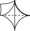
$S_{1}$ $S_{2}$ $S_{3}$ $S_{4}$ $S_{5}$

Figure 24. Quadrilateral in the Surface

Proof.

To prove Proposition 41 we must prove the following lemma.

Lemma 42.

If $\lambda$ and $\hat{\lambda}$ are $\alpha$-simple ideal triangulations of $S$, there exists a sequence of $\alpha$-simple ideal triangulations $\lambda=\lambda^{0},\lambda^{1}$ ,…, $\lambda^{m}$ such that $\lambda^{l+1}$ is obtained from $\lambda^{l}$ by a single diagonal exchange and a sequence of $\alpha$-simple ideal triangulations $\hat{\lambda}=\hat{\lambda}^{0}$ , $\hat{\lambda}^{1}$ ,…, $\hat{\lambda}^{n}$ such that $\hat{\lambda}^{l+1}$ is obtained from $\hat{\lambda}^{l}$ by a single diagonal exchange and four edges $K$ and $\hat{K}$ of $\lambda^{m}$ and $\hat{\lambda}^{n}$ respectively such that one component $C_{1}$ of $S-K$ and one component $\hat{C}_{1}$ of $S-\hat{K}$ are both spheres with four spikes at infinity. Also $\lambda^{m}$ and $\hat{\lambda}^{n}$ coincide outside of $C_{1}$.

Proof.

We will use the following proof for both $\lambda$ and $\hat{\lambda}$. Consider a quadrilateral as represented in Figure 24 with endpoints $S_{1},S_{2},S_{3},S_{4}$ where $S_{1},S_{2},S_{3},S_{4}$ are all points at infinity and the edge from $S_{1}$ to $S_{2}$ is a boundary curve and the edges in this quadrilateral are edges $S_{1}$ to $S_{2}$, $S_{1}$ to $S_{3}$, $S_{1}$ to $S_{4}$, $S_{2}$ to $S_{3}$ and $S_{3}$ to $S_{4}$. If $S_{1}=S_{2}$ then we are done. Assume from now on that $S_{1}\neq S_{2}$

Case 1: If $S_{3}=S_{1}$ and $S_{4}=S_{1}$ then doing a diagonal exchange on both $\lambda$ and $\hat{\lambda}$ in this quadrilateral lowers the number of edges ending at $S_{1}$ by one. Also since $\alpha$ cannot cross the edge connecting $S_{1}$ to $S_{2}$ when you do this diagonal exchange the resulting triangulation remains $\alpha$-simple.

Case 2: If $S_{1}=S_{3}$ and $S_{1}\neq S_{4}$, then doing a diagonal exchange on both $\lambda$ and $\hat{\lambda}$ in this quadrilateral lowers the number of edges ending at $S_{1}$ by two. Also, the resulting triangulation remains $\alpha$-simple.

Case 3: If $S_{1}\neq S_{3}$ and $S_{1}\neq S_{4}$, then doing a diagonal exchange on both $\lambda$ and $\hat{\lambda}$ in this quadrilateral decreases the number of edges ending at $S_{1}$ by one. Also, the resulting triangulation remains $\alpha$-simple.

Case 4: If $S_{1}\neq S_{3}$ and $S_{1}=S_{4}$. then after doing a diagonal exchange on both $\lambda$ and $\hat{\lambda}$ in this quadrilateral if we consider the new quadrilateral created with edges $S_{1}$ to $S_{2}$, $S_{2}$ to $S_{4}$, $S_{1}$ to $S_{4}$ and a new point $S_{5}$ and edges $S_{1}$ to $S_{5}$ and $S_{4}$ to $S_{5}$ then we see that we are again in Case 2 or Case 3. Thus after another diagonal exchange on both $\lambda$ and $\hat{\lambda}$ in this new quadrilateral we reduce the number of edges ending at $S_{1}$ by one or two. For the same reason as above after the first diagonal exchange the resulting triangulation remains $\alpha$-simple and similarly after the second diagonal exchange the resulting triangulation remains $\alpha$-simple.

Now if we repeat this process until there are only two edges going to $S_{1}$ then we can effectively “forget” about the point at infinity $S_{1}$ and then repeat this process for another point at infinity. By the method of the proof we automatically get $\lambda^{m}$ and $\hat{\lambda}^{n}$ to coincide outside of $C_{1}$.

If we continue this process for each of the four wide holes of $S$ then we are left with spheres with four spikes at infinity. By the method of the proof we automatically get $\lambda^{m}$ and $\hat{\lambda}^{n}$ to coincide outside of $C_{1}$.

∎

Lemma 43.

After changing the ideal triangulation $\lambda$ by $\alpha$-simple diagonal exchanges, we can arrange so that the following hold:

1. $\lambda$ satisfies the conditions of Lemma 42, namely there exists four edges $K$ such that one component $C_{1}$ of $S-K$ is a sphere with four spikes at infinity as represented in Figure 25.

2. Only two edges of $\lambda$ cross $\alpha$

3. $\alpha$ splits $C_{1}$ into two components, each of which contains four edges that are disjoint from $\alpha$ and two boundary edges.

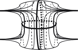
$\alpha$

Figure 25. Triangulation of the Sphere

Proof.

For the first condition we simply apply Lemma 42 to $\lambda$.

The second condition can be realized using moves similar to those represented in Figure 26. The third condition follows from the second condition. ∎

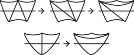
$\alpha$ $\alpha$

Figure 26. Reducing Crossings for the Sphere

Applying Lemma 42 and 43, we can assume without loss of generality that $\lambda$ and $\hat{\lambda}$ satisfy the conclusions of Lemma 43. By inspection, the two edges of $\lambda$ that cross $\alpha$ must go to a single boundary component of $C_{1}$ on one side of $\alpha$, and to a single boundary component of $C_{1}$ on the other side of $\alpha$.

Using the moves illustrated in Figure 27 we can arrange that the edges $A$ and $B$ of $\lambda$ and $\hat{\lambda}$ crossing $\alpha$ go to the same boundary components of $C_{1}$.

Finally, by using the moves represented in Figure 28, we can arrange that the two edges $A$ and $B$ wrap around $\alpha$ the same number of times. An application of the moves illustrated in Figure 29 ensures that $A$ and $B$ wrap around the boundary components of $C_{1}$ the same number of times.

After these moves the two ideal triangulations now coincide.

All of this argument also works for the surface $S$ that is obtained from the compact surface of genus zero with $k$ boundary components by removing $p$ points from its interior and at least one point from each boundary component, with $k+p=4$. In fact, some of the arguments become simpler.

∎

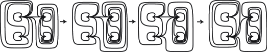
Figure 27. Changing Spikes in the Sphere

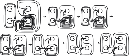
Figure 28. Changing Windings in the Sphere

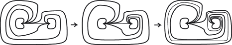
Figure 29. Diagonal Exchange Moves in the Sphere

We now prove Theorem 39 which we restate for the sake of the reader.

Theorem 44.

Let $S$ be a sphere with four holes. There exists a family of $T_{\alpha}^{\lambda}\in\mathcal{T}_{\lambda}^{q^{\frac{1}{4}}}(\alpha)$, with $\lambda$ ranging over all ideal triangulations of $S$ and $\alpha$ over all non-separating simple closed curves of $S$, which satisfies:

1. If $\alpha$ is in $\Sigma(S)$ and $\lambda$ and $\hat{\lambda}$ are two triangulations of $S$, then $\Theta_{\lambda\hat{\lambda}}(T_{\alpha}^{\hat{\lambda}})=T_{\alpha}^{\lambda}$.

2. as $q\rightarrow 1$, $T_{\alpha}^{\lambda}$ converges to the non-quantum trace function $T_{\alpha}$ in $\mathcal{T}(S)$

3. If $\alpha$ and $\beta$ are disjoint, $T_{\alpha}^{\lambda}$ and $T_{\beta}^{\lambda}$ commute.

4. If $\alpha$ meets each edge of $\lambda$ at most once then $T_{\alpha}^{q}$ is obtained from the classical trace $T_{\alpha}$ of Section 2.3 by multiplying each monomial by the Weyl ordering coefficient.

$\alpha$ $\beta$ $\alpha\beta$ $\beta\alpha$ $\gamma_{1}$ $\gamma_{2}$ $\gamma_{3}$ $\gamma_{4}$

Figure 30. Resolving Crossings in the Sphere

Proof.

The proof is identical to the proof of Theorem 33 replacing Proposition 30 with Proposition 41. ∎

We conclude with the proof of Theorem 40, which we repeat here for the convenience of the reader.

Theorem 45.

The traces $T_{\alpha}^{\lambda}$ of Theorem 44 satisfy the following property:

If $\alpha$ and $\beta$ meet in two points, and if $\alpha\beta$ and $\beta\alpha$ are obtained by resolving the intersection point as in Figure 30, then

$$T_{\alpha}^{\lambda}T_{\beta}^{\lambda}=qT_{\alpha\beta}^{\lambda}+q^{-1}T_{\beta\alpha}^{\lambda}+T^{\lambda}_{\gamma_{1}}T^{\lambda}_{\gamma_{2}}+T^{\lambda}_{\gamma_{3}}T^{\lambda}_{\gamma_{4}}$$

, for all $\lambda$

In addition, $T_{\alpha}^{\lambda}$, with $\alpha$ non-separating, is the only one which satisfy this property and conditions (1) and (4) of Theorem 44.

Proof.

Property (1) from Theorem 44 implies that it suffices to show $T_{\alpha}^{\lambda}T_{\beta}^{\lambda}=qT_{\alpha\beta}^{\lambda}+q^{-1}T_{\beta\alpha}^{\lambda}+T^{\lambda}_{\gamma_{1}}T^{\lambda}_{\gamma_{2}}+T^{\lambda}_{\gamma_{3}}T^{\lambda}_{\gamma_{4}}$ for one particular $\lambda$. Let $\lambda$ be the ideal triangulation as illustrated in Figure 31. The triangulation is $\alpha$-simple, $\beta$-simple, $\alpha\beta$-simple, but not $\beta\alpha$-simple.

The quantum traces $T_{\alpha}^{\lambda}$, $T_{\beta}^{\lambda}$ and $T_{\alpha\beta}^{\lambda}$ are determined by Condition 4 of Theorem 44. To compute $T_{\beta\alpha}^{\lambda}$, we use the triangulation $\hat{\lambda}$ of Figure 32 and use Condition 4 of Theorem 44 to determine $T_{\beta\alpha}^{\hat{\lambda}}$ and compute $T_{\beta\alpha}^{\lambda}=\Theta_{\hat{\lambda}\lambda}(T_{\beta\alpha}^{\hat{\lambda}})$

At this point checking the relation $T_{\beta\alpha}^{\lambda}=\Theta_{\hat{\lambda}\lambda}(T_{\beta\alpha}^{\hat{\lambda}})$ unfortunately requires considering $476$ terms. This computation was verified using Mathematica.

∎

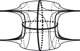
$\alpha$ $\beta$

Figure 31. $\alpha$-simple, $\beta$-simple, $\alpha\beta$-simple, but not $\beta\alpha$-simple Triangulation

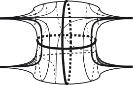
$\alpha$ $\beta$

Figure 32. $\beta\alpha$-simple Triangulation

References

- [1] H Bai, A Uniqueness Property For the Quantization of Teichmüller Spaces, to appear in Geometirae Dedicata, arXiv:mathGT/0509679 v1.
- [2] F Bonahon, X Liu, Representations of the quantum Teichmüller space and invariants of surface diffeomorphisms, Geo. Top. 11 (2007) 889-937
- [3] L O Chekhov, V V Fock, Observables in 3D Gravity and Geodesic Algebras, from: “Quantum groups and integrable systems (Prague, 2000)”, Czechoslovak J. Phys. 50 (2000) 1201-1208 MR1806262
- [4] M Culler, P B Shalen, Varieties of group representations and splittings of -manifolds, Ann. of Math. 117 (1983) 109-146
- [5] W M Goldman, Invariant functions on Lie groups and Hamiltonian flows of surface group representations, Invent. Math. 85 (1986) 263-302
- [6] R Kashaev, Quantization of Teichmüller spaces and the quantum dilogrithm, Lett. Math. Phys. 43 (1998) 105-115 MR1434238
- [7] X Liu, The Quantum Teichmüller Space as a Noncommutative Algebraic Object, arXiv:math.GT/0408361
- [8] F Luo, Geodesic length functions and Teichmüller spaces, J. Diff. Geo. 48 (1998) 275-317
- [9] F Luo, Grothendieck’s reconstruction principle and 2-dimensional topology and geometry, Commun. Contemp. Math 1 (1999) 125-153
- [10] R C Penner, The decorated Teichmüller space of punctured surfaces, Commun. Math. Phys. 113 (1987) 299-339 MR919235
- [11] W P Thurston, Three-Dimensional Geometry and Topology: Vol. 1, Princton Mathematical Series 35, Princeton University Press, Princton, NJ (1997) MR1435975 Edited by S Levy
- [12] V Turaev, Skein quantization of Poisson algebras of loops on surfaces, Ann. Sci. Ecol. Norm. Sup. (4) 24 (1991) 635-704 MR1142906