Star Formation Rates and Metallicities of $K$-selected Star Forming Galaxies at $z\sim 2$

Abstract

We present spectroscopy of 15 star-forming BzK galaxies (sBzKs) with $K_{\rm AB}\lesssim 23$ in the Subaru Deep Field, for which ${\rm H}\alpha$ and some other emission lines are detected in 0.9 to 2.3 $\micron$ spectra with a resolution of $R$=500. Using ${\rm H}\alpha$ luminosities, we obtain star formation rates (SFRs), and then specific SFRs (SSFRs) dividing SFRs by stellar masses, which are derived from SED fitting to $BVRi^{\prime}z^{\prime}K$ photometry. It is found that sBzKs with higher stellar masses have larger SFRs. A negative correlation is seen between stellar mass and SSFR, which is consistent with the previous results for $z\sim 2$ galaxies. This implies that a larger growth of stellar mass occurs in less massive galaxies. In addition, gas-phase oxygen abundances, 12+log(O/H), are derived from the ratio of [N II]($\lambda 6584$) to ${\rm H}\alpha$ using the N2 index method. We have found a correlation between stellar mass and oxygen abundance in the sense that more massive sBzKs tend to be more metal rich, which is qualitatively consistent with the relation for UV-selected $z\sim 2$ galaxies. However, the metallicity of the sBzKs is $\sim 0.2$ dex higher than that of UV-selected galaxies with similar stellar masses, which is significant considering the small uncertainties. The sBzKs in our sample have redder $R-K$ colors than the UV-selected galaxies. This galaxy color-dependence in the oxygen abundance may be caused by older or dustier galaxies having higher metallicities at $z\sim 2$.

1 Introduction

Recent studies suggest that the era of $z\sim 2$ is a turning point in galaxy formation and evolution. The cosmic star formation rate (SFR) begins to drop at $z\sim 1-2$ from a flat plateau at higher redshifts (Dickinson et al., 2003; Fontana et al., 2003; Ly et al., 2007). Significant evolution of the Hubble sequence occurred at $z\sim 1-2$ (Kajisawa & Yamada, 2001). It is also found that the number density of QSOs has a peak at $z\sim 2$ (Richards et al., 2006). These facts suggest that dramatic changes in the galaxy population occurred at $z\sim 2$, which are important to study in further detail.

Galaxy properties are determined from spectral characteristics such as emission lines, absorption lines and strong continuum breaks. At $z\sim 2$, the strongest of these features fall in the near-ultraviolet (NUV) and near-infrared (NIR) wavebands. NUV and NIR observations are thus essential to reveal detailed properties of $z\sim 2$ galaxies, but these observations encounter many difficulties, including poor sky transparency except for some atmospheric windows, and strong OH airglow emission lines and thermal emission from the atmosphere. This is why the era of $z\sim 2$ had been called a ‘redshift desert’ until recently. However, recent advances in wide-field imaging in the NUV and NIR, along with multi-object spectrographs, are beginning to fill in this ‘desert’ (e.g., Subaru Deep Field (SDF) survey, GOODS-North and South, UKIDSS, GMASS, and MUSYC (McCarthy et al., 1999; Reddy et al., 2006b; Erb et al., 2006c; Hayashi et al., 2007; Daddi et al., 2007; Grazian et al., 2007; Lane et al., 2007; Halliday et al., 2008; Kriek et al., 2008; Ly et al., 2008)).

A photometric selection technique using $B-z$ and $z-K$ colors has been proposed to choose an unbiased sample of $z\sim 2$ galaxies (BzK galaxies: Daddi et al. (2004)). Using these colors to find galaxies with a Balmer break between $z$ and $K$, the selected galaxies are then classified into star forming galaxies (sBzKs) and passively evolving galaxies (pBzKs). Thanks to wide and deep imaging surveys in the NIR as well as the optical, large new BzK samples are enabling us to measure their statistical properties, such as clustering strength (Kong et al., 2006; Hayashi et al., 2007; Blanc et al., 2008). The multiwavelength data also show that sBzKs are very actively forming stars(Dannerbauer et al., 2006; Daddi et al., 2007). On the other hand, due to lack of spectroscopic observations, there are relatively few accurately known redshifts, which are needed to derive accurate stellar masses and star formation rates from SED fitting to the multiwavelength data. Also, their physical properties such as metallicity are still not well-known.

More spectroscopy has recently become available for $z\sim 2$ galaxies selected by their UV colors. Erb et al. (2006a, b) presented a mass-metallicity ($M$-$Z$) relation and SFRs for UV-selected galaxies at $z\sim 2$ using 114 NIR spectra. They found a $M$-$Z$ correlation at $z\sim 2$ as there is in the local universe, with the more massive galaxies being more metal rich. Although the correlation has a similar slope to the local one, it is shifted to lower metallicity by $\sim 0.3$ dex. They have also found that SFRs derived from ${\rm H}\alpha$ luminosities are in good agreement with those from de-reddened rest-UV luminosities, with an average dust-corrected SFR of $\sim 30M_{\odot}{\rm yr^{-1}}$.

However, the rest-UV color selection misses about half of $z\sim 2$ galaxies, which have a large amount of dust extinction (Kong et al., 2006). The spectroscopic properties of this dusty population have yet not been clearly revealed. $K$-limited samples are better suited than UV-limited ones to investigate the relations between stellar mass and other fundamental properties at $z\sim 2$, because they approximately correspond to samples limited by stellar mass, without excluding galaxies with large dust extinction. Kriek et al. (2008) carried out a NIR spectroscopic survey for $K$-bright galaxies at $z\sim 2.3$. They suggest that studies with broadband photometric data alone may overestimate the number of massive galaxies at $z\sim 2$, and underestimate the evolution of the stellar mass density, again indicating the importance of spectroscopy.

In this paper, we present NIR spectroscopy for 44 BzK galaxies in the SDF, and their spectroscopic properties. The structure of this paper is as follows. The photometric and spectroscopic data are described in §2. In §3, we examine the properties of the detected emission lines, including spectroscopic redshifts and fluxes. We then investigate active galactic nuclei (AGN) contamination in our spectroscopic sample in §4. In §5, physical properties are derived from the emission lines, and then discussed. A summary is given in §6. Throughout this paper, magnitudes are in the AB system, and we adopt cosmological parameters of $h=0.7$, $\Omega_{m0}=0.3$ and $\Omega_{\Lambda 0}=0.7$.

2 Data

2.1 BzK galaxies in the SDF

Here we briefly describe the imaging data and sample selection of BzKs in the SDF, which are almost the same as those in Hayashi et al. (2007). The SDF is a large “blank” field centered on ($13^{\rm h}24^{\rm m}38\fs 9$, $+27\arcdeg 29\arcmin 25\farcs 9$; J2000), a rectangle of $29\farcm 7\times 36\farcm 7$, with deep multiwavelength data from the NUV to mid-IR (MIR) wavebands. Among these data, the optical and the NIR data are mainly used in this study. The optical data, $B$, $V$, $R$, $i^{\prime}$, $z^{\prime}$, NB816, and NB921, were obtained with the Suprime-Cam on the Subaru telescope for the Subaru Deep Field Project (Kashikawa et al., 2004), and then the NIR data, $J$ and $K$, were obtained with the wide field camera (WFCAM) on the United Kingdom Infra-Red Telescope (UKIRT) (Motohara et al. in preparation). The NIR data available to this study were only what was obtained on 2005 April 14 and 15, which limited the overlapping area with the optical data to about $40\%$ of the whole SDF (Hayashi et al., 2007). The $3\sigma$ limiting magnitudes in a $2\arcsec$-diameter aperture are 28.45 magnitude for $B$, 26.62 for $z^{\prime}$, and 24.05 for $K$. The optical images have been convolved to a seeing size of $1\farcs 14$, which is the value for $K$.

MIR data, 3.6 – 8.0 $\micron$, were obtained with the InfraRed Array Camera (IRAC) on the Spitzer space telescope. Since the point spread functions in the MIR data are much broader than those in optical and NIR data, some galaxy images are blended with nearby objects. For these, we had to remove the contaminating flux contributions from close objects in order to do accurate photometry. To do this we use GALFIT (Peng et al., 2002) to deblend images with adjacent objects (Hayashi et al. in preparation), and accurately measure the MIR fluxes of objects. The $3\sigma$ limiting magnitudes are 23.60 for $3.6\micron$, 23.32 for $4.5\micron$, 21.65 for $5.8\micron$, and 20.99 for $8.0\micron$, which are measured with $4.4\arcsec$, $4.4\arcsec$, $5.0\arcsec$, and $6.4\arcsec$ diameter apertures, respectively.

We applied the $BzK$ color selection proposed by Daddi et al. (2004) to the $B$, $z^{\prime}$, and $K$ data in the 180 arcmin² of the SDF which have good detection uniformity in all three passbands. In selecting BzK galaxies, deep optical data are crucial, because objects without $B$ or $z^{\prime}$ detections can take arbitrary positions on the $BzK$ color diagram, with almost all of them left unclassified. We selected the BzKs with great care for the optically undetected objects (See also Hayashi et al. (2007)). We obtained samples of 1092 sBzKs and 56 pBzKs with $K<23.2$, corresponding to the $5\sigma$ limiting total magnitude.

2.2 Spectroscopic observation

NIR spectroscopy of the BzKs in the SDF was carried out with the Multi-Object InfraRed Camera and Spectrograph (MOIRCS; Ichikawa et al., 2006) on the Subaru telescope on 2007 May 3 and 4. MOIRCS has a wide field of view of $4\arcmin\times 7\arcmin$, and its $zJ500$ and $HK500$ grisms provide spectra with a resolution of $R$=500, covering wavelengths of 0.9 – 1.8 $\micron$ and 1.3 – 2.5 $\micron$, respectively. The dispersions of the grisms are 5.57 and 7.72 Å/pixel, respectively.

Forty-four spectroscopic targets were selected from the samples of 1092 sBzKs and 56 pBzKs. We gave priority to $K<22.0$ BzKs in our samples for slitmask design, and then $K>22.0$ BzKs were allocated to the blank remaining slits. We used two slitmasks to cover the 44 BzKs, that is, each slitmask covers 22 BzKs. Each slit has a width of $0\farcs 7$ with a length of 10 – 12 $\arcsec$ according to the space between the slits. Among the 44 galaxies, 40 are classified as sBzKs and 4 as pBzKs. Half of them are fainter than $K=22.0$. Figure 1 shows the colors of the 44 BzKs.

We observed them consecutively at two positions (A and B) on the slit, using the $zJ500$ and $HK500$ grisms for one slitmask per night with single exposure times of 600 or 900 sec. The total on-source integration time was then 2 – 2.6 hours for both grisms. During the two nights, the weather was good, and the seeing was as good as $\sim 0\farcs 4$ in $K$, except for the end of May 4, when it was $\gtrsim 1\farcs 0$. We also observed A0 stars with $V\sim 9.0$ magnitude at different air masses with both grisms on each night to correct for the telluric absorption and the instrumental efficiency. Before and after the observations, dome flats with lamps on and off, and Th-Ar lamp data were obtained for wavelength calibration.

Figure 1: The colors of 44 targets. The filled circles are BzKs with $K<22.0$, and the filled triangles are those with $K>22.0$. BzKs with emission lines detected are squares.

2.3 Data Reduction

Data reduction is done with standard IRAF procedures. First, we create A – B frames from successive frames observed at the two positions. The A – B frames are then divided by a flatfield image, and bad pixels and cosmic rays are removed. The flat image is created by taking difference between the dome flat frames with the lamps on and off, and normalizing it. Next, distortion is corrected using calibration data files provided by the MOIRCS instrument team. Wavelength calibration is done with only the OH airglow lines for the $HK$ data, since there are numbers of the strong OH lines in the wavelengths longer than $1.1\micron$. On the other hand, for the $zJ$ data, Th-Ar data are also used for wavelength calibration at wavelengths shorter than $1.1\micron$. The wavelength uncertainties in the strong lines are less than 15Å.

Residual sky subtraction is then carried out, since only the A – B procedure may not completely remove the sky background due to its time variation. The telluric absorption and the instrumental efficiency are corrected using the spectra of A0 stars and the stellar spectral library given by Pickles (1998). Finally, all the frames for each galaxy are added and 1D spectra are extracted combining 5 pixels along a slit.

Flux calibration of the spectra is done using the photometry from the imaging data in $z^{\prime}$ and $K$. The $1\sigma$ error of the spectrum is estimated from the standard deviation in the sky region of the 2D spectrum.

3 Measurement of emission lines

3.1 Detection of emission lines

We have detected ${\rm H}\alpha$ and some other emission lines in 15 of the 40 sBzKs, 9 of which have $K>22.0$. Since there are many strong OH airglow lines in the NIR region, we have first confirmed all lines in the 2D spectra by visual inspection. Among the confirmed lines, then, we regard lines with a peak flux larger than the $3\sigma$ sky noise as a detection using 1D spectra with a resolution of $R$=500, that is, unbinned spectra. For the 4 pBzKs, no spectra with enough S/N to detect any Balmer/4000Å break were obtained due to the insufficient exposure times. In what follows, we examine and discuss spectroscopic properties of the 15 sBzKs with emission lines detected. Figures 2 – 4 show the binned 1D spectra of the lines, and Tables 1 and 2 show properties of the 15 sBzKs.

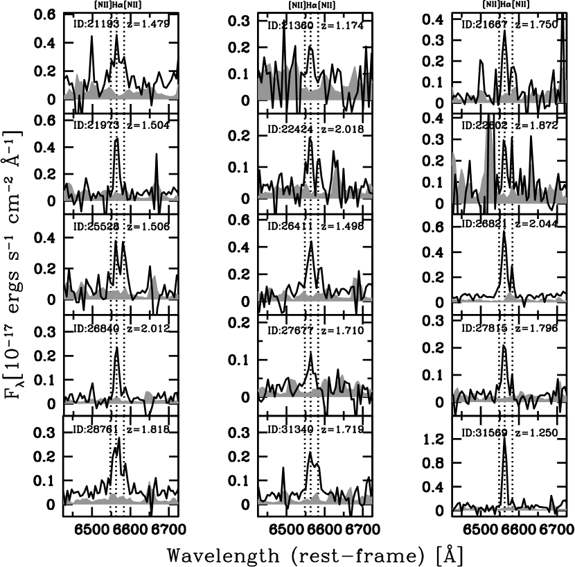
Figure 2: The spectra of ${\rm H}\alpha$ and [N II] emission lines we have detected. These spectra have a binned dispersion of $\sim 16$ Å. The solid lines show the spectra and the shaded regions in gray are the $1\sigma$ sky noise. We regard lines with a peak flux larger than the $3\sigma$ sky noise as a detection using unbinned 1D spectra. Labeled redshifts are derived from ${\rm H}\alpha$ lines.

To measure spectroscopic redshifts and fluxes of the emission lines, Gaussian profiles with a constant continuum are fitted, where the free parameters are amplitude, line width, redshift, and continuum level. The $1\sigma$ error of the spectrum is used as a sigma in the calculation of $\chi^{2}$. Because ${\rm H}\alpha$ ($\lambda$6563) and [N II] ($\lambda\lambda$6548,6584) are blended, they are simultaneously fitted, assuming the same line width and redshift, and a 6584/6548 ratio of 3-to-1. The $1\sigma$ error of each parameter in the fitting is estimated as the range where the increase in $\chi^{2}$ from the best-fit value is less than the appropriate value for the number of degrees of freedom (see §14.5 of Numerical recipes by Press et al. (1995)).

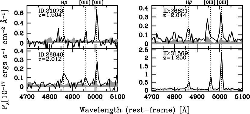
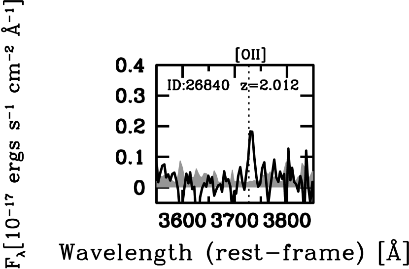
Figure 3: Same as Fig. 2, but for ${\rm H}\beta$ and [O III].

Figure 4: Same as Fig. 2, but for [O II].

3.2 Spectroscopic redshifts

Spectroscopic redshifts are derived from the ${\rm H}\alpha$ lines using the central wavelength of the fitted Gaussian. For four sBzKs, which are ID21360, ID21667, ID22602, and ID27677, only one emission line is detected, but we regard it as ${\rm H}\alpha$ for the following reasons: (1) The redshift of ID21360 is also confirmed to be 1.174 by optical spectroscopy with the Hectospec on the Multiple Mirror Telescope (Ly et al., 2008). Therefore, the line is certainly ${\rm H}\alpha$. (2) For the other three objects, it is possible that the detected lines, seen in the $HK$ grism spectra, are from transitions other than ${\rm H}\alpha$. If the lines are ${\rm H}\alpha$, the redshifts should be 1.75, 1.87, and 1.71, respectively. On the other hand, if the lines are [O III]($\lambda$5007), those would be 2.60, 2.76, and 2.55, respectively. The transition of ${\rm H}\beta$ would result in even higher redshifts. Then, because the BzK technique isolates selecting star forming galaxies at $1.4\lesssim z\lesssim 2.5$ by detecting the Balmer break between the $z$-band and $K$, ${\rm H}\alpha$ is the most likely identification of lines in the $HK$ region. (3) In addition, we note that almost all the derived spectroscopic redshifts are consistent with photometric redshifts. The photometric redshifts are obtained by fitting template SEDs to $BVRi^{\prime}z^{\prime}K$ photometric data using the Hyper$z$ code (version 1.1) (Bolzonella et al., 2000). The used set of template SEDs is what is provided in the Hyper$z$ package, which consists of the observed spectra based on the CWW templates (Coleman et al., 1980). The standard deviation of $\sigma(z_{\rm spec}-z_{\rm phot})$ is 0.61 for the 12 sBzKs with the secure spectroscopic redshfits. The photometric redshifts for ID21667 and ID22602 are 1.47 and 1.46, respectively, supporting our identification of their lines as ${\rm H}\alpha$. ID27677 would have a photometric redshift of 2.46, suggesting the possibility that the line is ${\rm H}\beta$ or [O III]. Since the flux ratio of [O III] to ${\rm H}\beta$ can widely range from 0.1 to 10 (Veilleux & Osterbrock, 1987), it is possible that only one of the two lines is detected. Note that [O III]($\lambda$4959) would not be detected due to the inadequate S/N even if the identification of [O III]($\lambda$5007) is correct. These considerations suggest that all the three of ${\rm H}\alpha$, ${\rm H}\beta$, and [O III] are candidates for the single line of ID27677, and that no secure conclusion is available for the line identification. Therefore, adopting the consideration (2), we assume that the line for ID27677 is also most likely to be ${\rm H}\alpha$. Even if the line is not ${\rm H}\alpha$, our conclusions discussed below would remain unchanged.

Since the spectral resolution is $R$=500, uncertainties in spectroscopic redshifts are estimated to be $\Delta z=\Delta\lambda_{\rm obs}({\rm H}\alpha)/6563\sim 0.002$.

Figure 5 shows the redshift distribution of the sBzKs with spectroscopic redshift, indicating a somewhat unexpected feature. The distribution does not peak at $z\sim 2$, and no object lies at $z>2$, contrary to the fact that $BzK$ color selection is proposed to select galaxies at $1.4<z<2.5$. In fact, Daddi et al. (2007) have reported that the redshift distributions of sBzKs with spectroscopic and photometric redshifts both peak at $z\sim 2$, and that this selection technique works well to select $z\sim 2$ galaxies, which is also supported by other results with photometric redshifts (Grazian et al., 2007; Blanc et al., 2008). The discrepancy of our result may be due to a flux-limited bias, or the fact that the strongest emission line, H$\alpha$, is shifted into a wavelength region of high sky background for $z>2$, as discussed in the next section. The opposite problem also occurs, namely that some galaxies at $z<1.4$ are selected, which are also seen in Fig. 2 of Daddi et al. (2007). These lower-$z$ objects are near the boundary of $BzK$ selection criterion, and lie 2.5 – 2.7 sigma from the color selection threshold. This result suggests that a fraction of star-forming galaxies at lower redshifts ($z<1.4$) can meet the sBzK criterion.

Figure 5: The redshift distribution of the sBzKs with spectroscopic redshift derived from the ${\rm H}\alpha$ lines. Errors are $\Delta z\sim 0.002$.

3.3 Objects without detected emission lines

Among the sBzK targets, no emission line is detected for 25 sBzKs. It is important to know the cause of the non-detections. Judging from the distribution of these sBzKs without a line detection on Figure 1, it is possible that they have large dust extinction. Applying equation (4) of Daddi et al. (2004) to the $B-z$ color, we find that sBzKs with $E(B-V)$ larger than $\sim 0.5$–which corresponds to Av=2.0 magnitude–have no lines detected. This may be one of the reasons for the non-detection of lines. Since there are many strong OH airglow lines in the NIR region, it is also possible that an emission line falls on a strong OH line. In addition, lines are redshifted into the $K$-band region in the case of $z>2$ sBzKs. As described in section 3.2, the S/N in the region may be too low for lines to be detected. In fact, there were no lines detected at a wavelength longer than $2.0\micron$. Finally, it is also possible that only sBzKs with higher SFRs have strong enough lines to be detected in this $K$-limited sample. The lowest ${\rm H}\alpha$ flux we detected is 4.2 $\times 10^{-17}$ ergs s^-1 cm^-2.

4 AGN contamination

Before considering the spectroscopic properties of sBzKs, we should account for possible AGN contamination in our sample. We use two methods to identify AGN candidates. One is the BPT emission-line diagnostic diagram (Baldwin et al., 1981), and the other is a power-law shaped SED from optical to MIR wavelengths.

Figure 6 is the emission-line diagnostic diagram showing the [O III]($\lambda$5007)/${\rm H}\beta$ vs. [N II]($\lambda$6584)/${\rm H}\alpha$ ratios. The only three sBzKs–ID26821, ID26840, and ID31569–have all the required lines detected. Undetected line fluxes for the other galaxies are estimated as follows. We derive ${\rm H}\beta$ fluxes from the ${\rm H}\alpha$ fluxes, $E(B-V)$ described in §5.1, and the assumed intrinsic Balmer decrement of ${\rm H}\alpha/{\rm H}\beta=2.86$. The fluxes of [O III] and [N II] are the $1\sigma$ upper limits derived from the sky noise at the wavelengths where each line should be seen, assuming the same line width as ${\rm H}\alpha$. As discussed in Kewley & Dopita (2002) and Erb et al. (2006a), the flux ratio of [N II]/${\rm H}\alpha$ is enhanced by shock excitation (in LINERs), or by the hard continuum which photo-ionizes the Narrow Line Region (NLR) of all Seyfert nuclei. Figure 7 in Kewley & Dopita (2002) shows that the ratio of [N II]/${\rm H}\alpha$ is always less than 0.63 in purely star-forming galaxies. Among the 15 spectroscopically confirmed sBzKs in our sample, four– ID21193, ID22424, ID25528, and ID31340–have [N II]/${\rm H}\alpha$ greater than 0.63, which may imply a significant contribution from either a LINER or Seyfert NLR component. In particular, ID25528 shows the high [N II]/${\rm H}\alpha$ ratio of 1.2, suggesting that it is an AGN. On the other hand, we cannot strongly assert that the other three galaxies are LINERs or Seyferts due to the uncertainties of their line ratios. Also, as described below, the SEDs suggest that their continuum is dominated by stellar emission, and that the AGN contribution is small. If they are type II AGNs, the strongest observed contribution to the spectrum from the active nucleus would be high-ionization emission lines, not continuum. Similarly, one galaxy–ID 31569–shows a high enough [O III]($\lambda$5007)/${\rm H}\beta$ ratio of 4.9 to be a possible Seyfert 2 galaxy. However, the weak [N II] line suggests that this is instead a metal-poor star-forming galaxy.

Figure 6: The emission-line diagnostic diagram showing the [O III]($\lambda$5007)/${\rm H}\beta$ vs. [N II]($\lambda$6584)/${\rm H}\alpha$ ratios. The solid line is the boundary separating star forming galaxies (left side) and AGNs (right side) (Kauffmann et al., 2003). Circles show objects identified as star forming galaxies, while a square and triangles as an AGN and possible AGN candidates, respectively. The undetected fluxes of [O III] and [N II] are estimated from the $1\sigma$ upper limits, which are shown by arrows. The ${\rm H}\beta$ fluxes are inferred from the ${\rm H}\alpha$ flux and $E(B-V)$ on the assumption of an intrinsic Balmer decrement of ${\rm H}\alpha/{\rm H}\beta=2.86$. The error bars are shown with $1\sigma$.

These ratios of forbidden to Balmer emission lines do not however provide a definitive search for AGN. This is because a strong contribution from the Broad Line Region (BLR) in Seyfert 1 nuclei produces a low [N II]/${\rm H}\alpha$ ratio which would not be noticeably different from those of H II regions. Our spectral resolution of 600 km s^-1 should be sufficient to detect most broad wing of ${\rm H}\alpha$, but no such wing is found. Furthermore, only one of the ${\rm H}\alpha$ lines–ID 26821–satisfies the criteria of Hicks et al. (2002) set for an Seyfert 1: EW $>$ 100Å and $\log L({\rm H}\alpha,{\rm observed})[{\rm ergs\ s^{-1}}]\geq 42.5$ (Table 2). This implies that there is a contribution from a Seyfert BLR component in ID26821 sBzK. However, as shown in §5.2.2, the SFR derived from ${\rm H}\alpha$ luminosity is in agreement with that from UV luminosity within a factor of 2, which may indicate that the contribution from a BLR to the ${\rm H}\alpha$ line is not significant.

We have also applied another test for Seyfert 1 nuclei in our sample. We checked the long-wavelength SEDs of the 15 sBzKs using the photometry from $3.6-8.0\mu m$ taken with IRAC on the Spitzer space telescope. Most of the sBzKs have a strong bump at a rest wavelength of 1.6 µm in their SEDs, indicating that their SEDs are dominated by stellar emission (Sawicki, 2002; Alonso-Herrero et al., 2007). AGN-dominated galaxies, especially those with broad emission lines (Seyfert 1’s) have a power-law SED at rest wavelengths longer than 1 µm (Malkan & Filippenko, 1983; Spinoglio et al., 1995). In our sample, no such clear power-law SEDs are seen, but three sBzKs have power-law-like SEDs: ID21973, ID26821, and ID27677 (Figure 7). These might perhaps contain ”Seyfert 1.9” or ”Narrow Line Seyfert 1” nuclei. However, intense star formation also produces substantial near-IR emission from heated dust, which could mimic such an SED. Figure 7 shows these three power-law-like SEDs with SED models of starbursts overplotted (SBURT: Takagi et al., 2003). These model SEDs have no contribution of AGN.

With all these considerations, we classify ID25528 and ID26821 as AGN. Although the AGN contribution to the spectra, particularly the continuum, may not be significant, the two galaxies are excluded from the discussions on emission lines in the following section. We then classify the three sBzKs of ID21193, ID22424, and ID31340 as AGN candidates judging from the [N II]/${\rm H}\alpha$ ratios. However, since it is possible that the three AGN candidates are star forming galaxies, we consider them as well as the other ten sBzKs classified as star forming galaxies in the following discussions.

Kong et al. (2006) have estimated that about 25% of sBzKs are AGNs using XMM-$Newton$ X-ray data, which would imply that 3 – 4 sBzKs in our sample could be AGN. However, the sample of Kong et al. (2006) has only $K$-bright BzKs. According to Alonso-Herrero et al. (2007), the characteristic stellar mass of the host galaxy of AGN increases with redshift, and at $z\sim 2$ it is $\sim(1-3)\times 10^{11}M_{\odot}$. In our sample, almost all galaxies are less than $10^{11}M_{\odot}$, which indicates that the fraction of AGN can be lower than 25%. The NICMOS imaging of Colbert et al (2005) also indicates that fewer than a quarter of these less massive galaxies should host an AGN detectable in X-rays. The AGN fraction of 2/15 (13%) in our sample is consistent with the number of AGN expected from other studies. If the three candidates are actually AGNs, the fraction increases to 33%, which would still be consistent with other studies.

Figure 7: The long-wavelength power-law-like SEDs of ID21973, ID26821, and ID27677 sBzKs, where model SEDs of starbursts (without any AGN contribution) from Takagi et al. (2003) are overplotted.

5 Properties of star-forming BzK galaxies

Emission line information enables us to estimate SFR and metallicity. In the local universe, more massive galaxies tend to have lower SFRs and higher metallicities (e.g., Gallazzi et al., 2005). It is important to examine whether a similar relation exists among these properties for high redshift galaxies.

In this section, we first describe the properties obtained from multiwavelength photometric data by SED fitting method. Then, spectroscopic properties are discussed, along with the photometric properties.

5.1 Properties from SED fitting

Properties such as stellar mass and dust extinction, $E(B-V)$, are obtained from fitting synthetic model spectra of continuous bursts (Bruzual & Charlot, 2003) to the $BVRi^{\prime}z^{\prime}K$ photometry, assuming a standard Salpeter (1955) initial mass function (IMF), solar abundance, and the empirical dust extinction of Calzetti et al. (2000). These are shown in Table 1. Stellar mass is one of the most important parameters of galaxy properties and the most robust one obtained from SED fitting. Although sBzKs are well-fitted by the continuous burst model, fits using the $\tau$ model, where the SFR declines exponentially with time, would make the stellar masses slightly smaller than those with the continuous burst model. Note that SEDs of the simple stellar population (SSP) model are irrelevant in this work, since sBzKs are still star-forming at $z\sim 2$. It is also noted that if a Chabrier (2003) IMF is used, stellar masses (and SFRs) are smaller by a factor of 1.8 than those with a Salpeter IMF. Thus, stellar masses are determined within a factor of $\sim 2.5$. Fitted $E(B-V)$s are mainly used to calibrate the dust extinction of emission line fluxes in section 5.2. As discussed in section 4, almost all SEDs of the sBzKs are dominated by stellar emission with a clear 1.6$\mu m$ bump. Therefore, any AGN contribution to the SED is small enough that parameters obtained from the SED fitting reflect properties of the stellar populations.

5.2 Star Formation Rates

5.2.1 SFR derived from H$\alpha$ and UV continuum

SFRs for sBzKs are derived from the luminosity of ${\rm H}\alpha$ using the equation given in Kennicutt (1998);

$${\rm SFR}_{{\rm H}\alpha}[M_{\odot}{\rm yr^{-1}}]=7.9\times 10^{-42}L_{{\rm H}\alpha}[{\rm ergs\ s^{-1}}],$$ (1)

assuming solar abundance, Salpeter IMF with mass limits of 0.1 and 100 $M_{\odot}$, and a constant SFR. ${\rm H}\alpha$ luminosities are corrected for the dust extinction by equation (3) in Calzetti et al. (2000), $E(B-V)=0.44E_{\rm gas}(B-V)$. The amount of nebular extinction is then estimated from $E_{\rm gas}(B-V)$ using the extinction law given in Calzetti et al. (2000). The median amount of extinction of ${\rm H}\alpha$ is 2.83 magnitude.

The amount of extinction at ${\rm H}\alpha$ can be directly estimated from the apparent ${\rm H}\alpha/{\rm H}\beta$ ratio. However, we do not apply this method for our sample, because only three galaxies have detection of both lines and even for these three the amount of extinction is not strongly constrained due to a large uncertainty in the ${\rm H}\beta$ flux.

The rest-UV luminosity is also used as a tracer of SFR. We derive SFR from the continuum at 1500Å, $L_{1500}$, which is predicted by the best-fit model to the $BVRi^{\prime}z^{\prime}K$ photometry. $L_{1500}$ is corrected for the dust extinction with Calzetti extinction law and converted into a SFR using the equation given in Daddi et al. (2004);

$${\rm SFR}_{\rm UV}[M_{\odot}{\rm yr^{-1}}]=\frac{L_{1500}[{\rm ergs\ s^{-1}\ Hz^{-1}}]}{8.85}\times 10^{-27}.$$ (2)

5.2.2 Comparison between ${\rm SFR}_{{\rm H}\alpha}$ and ${\rm SFR}_{\rm UV}$

Figure 8 compares the SFR from the rest-UV luminosity with that from ${\rm H}\alpha$. A correlation is seen between the two SFRs, but ${\rm SFR}_{{\rm H}\alpha}$ tends to be larger than ${\rm SFR}_{\rm UV}$ by a factor of three. The median ${\rm SFR}_{{\rm H}\alpha}$ and ${\rm SFR}_{\rm UV}$ are 182 and 61 $M_{\odot}{\rm yr^{-1}}$, respectively. Also, this discrepancy between SFR measured by ${\rm H}\alpha$ and from shorter wavelength observations is quite similar to what Hicks et al. (2002) found in their sample of IR-selected galaxies.

On the other hand, Erb et al. (2006b) report that ${\rm SFR}_{{\rm H}\alpha}$ for UV-selected $z\sim 2$ galaxies is in good agreement with ${\rm SFR}_{\rm UV}$, which is inconsistent with our result. However, their observed ${\rm H}\alpha$ luminosities are similar to ours. That is, the median ${\rm H}\alpha$ luminosities of our sample and that of Erb et al. (2006b) are 2.0 and 2.2 times $10^{42}$ ergs s^-1, respectively. This disagreement on resulting SFRs with Erb et al. (2006b) may be due to different corrections for dust extinction at ${\rm H}\alpha$. They used the color excess for the stellar continuum to de-redden ${\rm H}\alpha$, that is, $E_{\rm gas}(B-V)=E(B-V)$, which implies that their amount of dust correction for ${\rm H}\alpha$ luminosity is systematically lower than ours by 1.6 magnitude on average. This leads to a difference in derived SFRs of a factor of 4.4. Using the same method as Erb et al. (2006b) for de-reddening ${\rm H}\alpha$, our correlation between ${\rm SFR}_{{\rm H}\alpha}$ and ${\rm SFR}_{\rm UV}$ becomes consistent with that of Erb et al. (2006b). In this case, the median ${\rm SFR}_{{\rm H}\alpha}$ is 50 $M_{\odot}{\rm yr^{-1}}$.

Daddi et al. (2004) report that most color excesses of 24 sBzKs in the K20/GOODS area, which are derived from $U$ to $K$ SEDs, fall within a range of $0.2\lesssim E(B-V)\lesssim 0.5$, which is consistent with our result (Table 1). The median $E(B-V)$ in our sample is 0.38. This implies that our estimation of $E(B-V)$ by SED fitting is reliable.

This difference between ${\rm SFR}_{{\rm H}\alpha}$ and ${\rm SFR}_{\rm UV}$ implies two possibilities. One is that a Salpeter IMF is unsuitable, if the equation of Calzetti et al. (2000), $E(B-V)=0.44E_{\rm gas}(B-V)$, is assumed to be valid for star-forming galaxies at $z\sim 2$. A more top-heavy IMF than Salpeter would account for the difference, since nebular emission results from ionizing photons shortward of the Lyman limit. The other is that the equation of Calzetti et al. (2000) cannot be applied to $z\sim 2$ galaxies. In any case, in what follows we use ${\rm SFR}_{{\rm H}\alpha}$ for sBzKs in the comparison with their stellar masses. Even if ${\rm SFR}_{\rm UV}$ were used instead, the discussion in the next section would remain unchanged.

Figure 8: Comparison between ${\rm SFR}_{{\rm H}\alpha}$ and ${\rm SFR}_{\rm UV}$. ${\rm SFR}_{{\rm H}\alpha}$s are derived from ${\rm H}\alpha$ luminosities, and then ${\rm SFR}_{\rm UV}$s are from the luminosities at 1500 Å  estimated from the best-fitted SEDs. Both SFRs are corrected for dust extinction. The dotted line shows that ${\rm SFR}_{\rm UV}$ is equal to ${\rm SFR}_{{\rm H}\alpha}$.

5.2.3 Relation to stellar mass

We examine the relation between ${\rm SFR}_{{\rm H}\alpha}$ and stellar mass. Figure 9 suggests that sBzKs with higher stellar masses have larger SFRs, which is qualitatively consistent with Daddi et al. (2007). However, the slope of our relation is shallower than theirs. One cause for this disagreement in the slope may be a difference between ${\rm SFR}_{{\rm H}\alpha}$ and ${\rm SFR}_{\rm UV}$. Figure 8 suggests the difference between these two estimates of SFR is larger at lower SFRs. Since less massive sBzKs have lower SFRs, this difference results in shallower slope of the correlation between stellar mass and ${\rm SFR}_{{\rm H}\alpha}$. Other cause may be a difference in the method used to derive stellar masses. Daddi et al. (2007) have used the empirical relation between the stellar mass and $K$ given in Daddi et al. (2004), which is calibrated based on $z-K$ color. We compare the stellar masses derived from a SED-fitting with those from the relation of Daddi et al. (2004), finding that the difference between the two estimates of stellar mass is larger at smaller stellar mass. The stellar masses from the relation are larger by a factor of 2 – 3 in $\sim 10^{10}M_{\odot}$. Because this relation is derived using bright $K<22$ BzKs, the stellar masses of faint BzKs may be overestimated compared with those from SED fitting, resulting in the shallower correlation between stellar mass and ${\rm SFR}_{{\rm H}\alpha}$.

It is also possible that a flux-limited bias, discussed in §§3.2 and 3.3, produces this disagreement. If galaxies with $\left<E(B-V)\right>=0.38$ and $F({\rm H}\alpha)=4.2\times 10^{-17}{\rm ergs\ s^{-1}\ cm^{-2}}$, which is the lowest ${\rm H}\alpha$ flux we have detected, are at $\left<z\right>\sim 1.7$, the SFR would be $\sim 87M_{\odot}{\rm yr^{-1}}$. This suggests that it is likely that we cannot detect any emission lines for galaxies with SFR $\lesssim$ 87 $M_{\odot}{\rm yr^{-1}}$. Moreover, it is found that ${\rm SFR}_{{\rm H}\alpha}$s is three times larger than ${\rm SFR}_{\rm UV}$s on average. Combining this with the relation between stellar mass and ${\rm SFR}_{\rm UV}$ given in Fig. 17 of Daddi et al. (2007), we find that the limiting SFR of 87 $M_{\odot}{\rm yr^{-1}}$ corresponds to a stellar mass of $\sim 1\times 10^{10}M_{\odot}$. These estimates indicate that it is possible that no galaxies with $\lesssim 1\times 10^{10}M_{\odot}$ and $\lesssim 87M_{\odot}{\rm yr^{-1}}$ are detected due to flux-limited bias. However, even if Figure 9 is limited to a region with SFRs higher than the estimated detection limit, a mild correlation between stellar mass and SFR can be seen. If there are less massive galaxies with lower SFRs, as found in Daddi et al. (2007), the correlation would be steeper.

Erb et al. (2006b) have also reported a similar correlation between SFR and stellar mass for UV-selected $z\sim 2$ galaxies, but their correlation is shifted to much lower SFR than ours. This is mainly due to differences in the assumed IMF as well as dust correction, as discussed in section 5.2.2. In Erb et al. (2006b), a Chabrier IMF is used to estimate stellar masses and SFRs. SFRs derived with a Chabrier IMF are smaller than those with a Salpeter IMF by a factor of 1.8. These differences make our SFR 7.9 times larger than that of Erb et al. (2006b). After correcting these systematic differences, the comparison of the results between sBzKs and UV-selected galaxies indicates that the former tend to have slightly higher SFRs than UV-selected galaxies with the similar stellar masses. This reflects the intrinsic difference between the the dust amount in the two populations–only sBzKs with higher SFRs may be easily detected, due to the larger dust extinction than in UV-selected galaxies.

The positive correlation between SFR and stellar mass may be attributed to a larger amount of gas in more massive galaxies, as suggested by Daddi et al. (2007).

Figure 9: The relation between ${\rm SFR}_{{\rm H}\alpha}$ and stellar mass. Stellar masses are derived from SED fitting to $BVRi^{\prime}z^{\prime}K$ photometry. The dotted line shows the limiting SFR of $87M_{\odot}{\rm yr^{-1}}$ estimated from the lowest detected flux on the assumption that the galaxy is at $<z>=1.7$ and suffer a typical color excess of 0.38.

5.2.4 Specific SFR

We derived specific SFRs (SSFRs) from ${\rm SFR}_{{\rm H}\alpha}$s and stellar Masses. SSFR is an indicator of the time scale of star formation activity. Figure 10 shows SSFR as a function of stellar mass. A negative relation is seen between stellar mass and SSFR, which is consistent with previous results for $z\sim 2$ galaxies (Reddy et al., 2006a; Erb et al., 2006b). This negative relation implies that a larger growth of stellar mass occurs in less massive galaxies. In comparison with Erb et al. (2006b), it should be noted that we apply a different IMF and dust correction as described in the previous section. In Figure 10, the results of Erb et al. (2006b) are converted into those with the same manner as ours.

We must consider the effect of flux-limited bias on this correlation, as discussed in the previous section. However, it seems that there is a genuine negative correlation even if the range of validity is limited to stellar masses larger than $1\times 10^{10}M_{\odot}$. The steep relation between stellar mass and SSFR results from the shallow correlation between stellar mass and SFR, which shows that the increase in SFR is not as rapid as that in stellar mass. If we miss galaxies with low SFRs of $\lesssim 87M_{\odot}{\rm yr^{-1}}$ as discussed in section 5.2.3, that is, the correlation between stellar mass and SFR is steeper, the relation with SSFR would be shallower than that in Figure 10.

Figure 10: The relation between the specific ${\rm SFR}_{{\rm H}\alpha}$ and the stellar mass. Filled circles are our results, open triangles show those of Reddy et al. (2006a) for sBzKs in their UV-selected sample, and crosses are those of Erb et al. (2006b) for UV-selected sample. All stellar masses and SSFRs are converted into those derived with Salpeter IMF and the same dust correction as we apply. The dotted line shows the track of galaxies with a constant SFR of 87$M_{\odot}{\rm yr^{-1}}$.

5.3 Equivalent Width

The rest-frame equivalent widths of ${\rm H}\alpha$ are derived from Gaussian fitting. Both ${\rm H}\alpha$ and continuum fluxes have been corrected for dust extinction. As discussed in Erb et al. (2006b), one can infer the star formation history of galaxies from the equivalent width. While the flux of ${\rm H}\alpha$ reflects the current star forming activity, the continuum flux emitted from stars reflects the past star formation. That is to say, the equivalent width represents how actively a galaxy is forming stars compared with the past. Thus, the equivalent width is a similar indicator to SSFR. Figure 11 shows the equivalent width as a function of the SSFR, indicating a mild correlation. This supports the result of the previous section. Less massive galaxies are more actively forming stars, which results in a larger growth of stellar mass.

Figure 11: The relation between specific star formation rate and ${\rm H}\alpha$ equivalent width in rest frame. Rest-frame equivalent widths of ${\rm H}\alpha$ are derived from line and continuum fluxes after correction for dust extinction.

5.4 Metallicity

Average metallicity is one of the most important properties of a galaxy. Since gas and stellar metallicities are related to the past star formation, they are crucial for understanding the star formation history and galaxy evolution. It is well-known that metallicity is correlated with stellar mass in the local universe (e.g., Tremonti et al., 2004). Erb et al. (2006a) have reported a similar correlation to the local one for UV-selected galaxies at $z\sim 2$. However, their mass-metallicity ($M$-$Z$) relation at $z\sim 2$ is shifted to lower metallicity by $\sim 0.3$ dex. This $M$-$Z$ relation at $z\sim 2$ obtained by Erb et al. (2006a) is widely used as representative of $z\sim 2$ star forming galaxies in comparison with both observational and theoretical studies (Liu et al., 2008; Maiolino et al., 2008; Brooks et al., 2007; De Dossi et al., 2007; Finlator & Dav$\rm\acute{e}$, 2008). However, because the UV selection misses star forming galaxies with a large dust extinction, we cannot be confident that the $M$-$Z$ relation of Erb et al. (2006a) applies to all star-forming galaxies at $z\sim 2$. Here, we determine a $M$-$Z$ relation for sBzKs. Our sBzK sample, which approximately corresponds to a stellar mass-limited sample, should be more suitable for deriving the $M$-$Z$ relation at $z\sim 2$.

It is well known that electron temperature reflects gas metallicity (Kewley & Dopita, 2002; Kobulnicky & Kewley, 2004; Erb et al., 2006a). Because auroral lines, which are used to derive electron temperature, are weak, and observed in only galaxies with low metallicities, it is very difficult even in local galaxies to estimate the metallicity of galaxies from them. We can only use the ratio of strong emission lines which are emitted from different ionization levels to derive metallicity for high-$z$ galaxies. At present, there are various metallicity diagnostics, such as the $R_{23}$ and N2 methods, to estimate gas-phase oxygen abundance, 12+log(O/H). One problem with these diagnostics is a disagreement between the resulting oxygen abundances inferred from the different diagnostics. Even if the same diagnostic is used, some different calibrations give a large difference in the resulting metallicities (Kewley & Dopita, 2002; Kobulnicky & Kewley, 2004). The same diagnostics and calibration should be used to properly compare with other results.

We derive 12+log(O/H) using the N2 index method proposed by Storchi-Bergmann et al. (1994), where N2 is defined as the flux ratio of [N II]($\lambda 6584$)/${\rm H}\alpha$;

$${\rm N2}\equiv\log\frac{[{\rm NII}](\lambda 6584)}{{\rm H}\alpha}.$$ (3)

The gas-phase oxygen abundances are derived with the following relation given in Pettini & Pagel (2004);

$$\begin{array}[]{l}12+\log({\rm O/H})=8.90+0.57\times{\rm N2}.\end{array}$$ (4)

The reasons we use this relation are that it requires only two lines of ${\rm H}\alpha$ and [N II], and the result can be compared directly with that of Erb et al. (2006a), where the same relation was used to derive the gas abundance. Also, it should be noted that the lines of ${\rm H}\alpha$ and [N II] are close enough that the difference in dust extinction is negligible. The $1\sigma$ dispersion in the abundance derived from the relation is 0.18 (Pettini & Pagel, 2004).

Figure 12 shows the resulting relation between stellar mass and metallicity. The broken line shows the abundance for galaxies with the flux ratio of [N II]/${\rm H}\alpha$=0.63, where N2 saturates (Kewley & Dopita, 2002), suggesting that the linear relation between the oxygen abundance and N2 index is acceptable up to the abundance of $\sim 8.79$. As discussed in section 4, the three sBzKs with a large abundance, ID21193, ID22424, and ID31340, may harbor AGNs, because they have flux ratios of [N II]/${\rm H}\alpha$ larger than 0.63. However, their SEDs suggest that their continuum is dominated by stellar emission, and that the AGN contribution is small. Even if the three AGN candidates are excluded from our sample, our conclusions in the following discussion are unchanged.

We derive upper limits of metallicity for sBzKs without a secure detection of [N II], assuming that the peak flux is 3 times sky noise, and that the line width is the same as that of ${\rm H}\alpha$. These galaxies are shown by crosses in the figure. Also, we estimate mean metallicity of the five sBzKs without [N II] detection. We derive it from the stacked spectrum using the equations (3) and (4), finding that the mean abundance is 8.55. This is shown by the double circle in the figure, whose stellar mass is the average of those of the five sBzKs.

Figure 12: Stellar mass vs. metallicity relation. Circles and crosses show our results. Filled circles show those of sBzKs with the detection of both ${\rm H}\alpha$ and [N II]. Crosses show upper limits of sBzKs without the detection of [N II], which are derived using the $3\sigma$ upper limit on [N II] flux. The double circle shows the mean abundance of the five sBzKs without a detection of [N II] against the mean stellar mass. Open squares show UV-selected $z\sim 2$ galaxies, and open triangles are those of the local $\sim 53,000$ SDSS galaxies (Erb et al., 2006a). All abundances are estimated using the same N2 index method. The dotted line is the solar oxygen abundance of 12+log(O/H)=8.66 (Asplund et al., 2004). The broken line shows the abundance for galaxies with the flux ratio of [N II]/${\rm H}\alpha$=0.63. Stellar masses of the Erb et al. (2006a) are converted into those derived with Salpeter IMF.

Figure 12 shows that more massive sBzKs tend to be more metal-rich, a trend qualitatively consistent with that of Erb et al. (2006a). However, the metallicities of sBzKs with [N II] detection are higher by $\sim 0.2$ dex than those of UV-selected galaxies with the same stellar mass at the similar redshift. Considering the uncertainties, a significant shift exists at the 2.7$\sigma$ level between the two $M$-$Z$ relations. If three AGN candidates are excluded from the sample, the confidence level in the shift slightly decreases, to the 1.8$\sigma$ level.

We again emphasize that the N2 flux ratios are converted into the oxygen abundances using the same relation as Erb et al. (2006a). We make sure that the N2 indices are larger than those of Erb et al. (2006a) for galaxies with the given stellar masses, suggesting that the cause of the difference in $M$-$Z$ relation is not a systematic difference in our abundance estimate methodology.

Pettini & Pagel (2004) have found a relation between gas oxygen abundance and O3N2 index, which is defined as ${\rm O3N2}$ $\equiv$ $\log$[([O III]($\lambda 5007$)/${\rm H}\beta$) / ([N II]($\lambda 6584$)/${\rm H}\alpha$)]. We check the abundance with the O3N2 diagnostics for three sBzKs with the necessary lines observed. The abundances from the O3N2 ratios are lower than those from the N2 ratios by $\sim 0.13$ dex. This is consistent with Erb et al. (2006a), who found that the abundances from O3N2 are 0.17 dex lower on average than those from N2. In addition, it is not likely that the systematic difference in estimates of stellar masses accounts for the difference in the $M$-$Z$ relation. The stellar masses of Erb et al. (2006a) are converted into those derived with Salpeter IMF. As discussed in section 5.1, the systematic difference of stellar masses should be less than a factor of 2. This indicates that there is no way that it is the cause of the difference in $M$-$Z$ relation.

We consider the possibility that our $M$-$Z$ relation suffers from a selection bias that only sBzKs with high metallicities are plotted, since metallicities are properly measured only for sBzKs with both ${\rm H}\alpha$ and [N II] lines detected. The stacking analysis for sBzKs without [N II] detection suggests that there are also sBzKs with lower metallicities (Figure 12), supporting the idea that selection bias cannot be completely ruled out. This may imply that the mean metallicities of sBzKs with given stellar masses are slightly lower than those plotted in Figure 12. However, the mean metallicity of only sBzKs without [N II] detection is similar to that of UV-selected galaxies, implying that sBzKs would still be more metal rich on average than UV-selected galaxies. This fact suggests that it is likely that the UV selection misses star forming galaxies at $z\sim 2$ with comparatively higher metallicities, and that metallicities of star forming galaxies at $z\sim 2$ have a large dispersion.

Therefore, we conclude that the oxygen abundance of sBzKs is greater than that of UV-selected $z\sim 2$ galaxies. As described in section 5.2, $K$-selected star forming galaxies at $z\sim 2$ have slightly higher SFRs but similar to UV-selected galaxies, if the same correction for dust extinction is applied, while their metallicities are significantly different. This fact may imply that the two star forming galaxy populations at $z\sim 2$ pass through different star forming histories before this epoch.

This difference in the $M$-$Z$ relation between sBzKs and UV-selected galaxies may be related to the difference in color of the two populations. Figure 13 shows $R-K$ color as a function of $K$ for our sBzK sample and the UV-selected galaxy sample of Erb et al. (2006a). This figure shows that the sBzK spectroscopic sample galaxies are redder than the UV-selected galaxies. Indeed, the sBzK ID31569, which is as blue as UV-selected galaxies, is located on the $M$-$Z$ relation of Erb et al. (2006a). The difference in $R-K$ color may imply that galaxies with different colors have different ages and/or dust contents, since the 4000Å break falls between the $R$ and $K$-bands. This fact indicates that star forming galaxies at $z\sim 2$ with redder colors have larger metal abundances, and that the $M$-$Z$ relation of Erb et al. (2006a) may not represent the entire population of $z\sim 2$ galaxies.

Another possibility is that the difference in redshifts of galaxies between the two samples accounts for the difference in the $M$-$Z$ relation. While the median redshift of galaxies in our sample is 1.7, the mean redshift is $\left<z\right>=2.2$ in the Erb et al. (2006a) sample. Because the galaxies in our sample are on average at a lower redshift, the fact that our sBzKs have higher metallicities than UV-selected galaxies of Erb et al. (2006a) may plausibly be attributed to cosmic evolution. However, this interpretation would require a surprisingly rapid evolution of the $M$-$Z$ relation over 800 Myr.

We plot results of star forming galaxies at $z\sim 0$ from SDSS data in Figure 12 (Tremonti et al., 2004; Erb et al., 2006a). It should be noted that we cannot directly discuss redshift evolution of the $M$-$Z$ relation, since these SDSS galaxies are not necessarily descendants of sBzKs. Our $M$-$Z$ relation seems to be similar to that of SDSS galaxies (Tremonti et al., 2004), but we may not necessarily claim that the metallicities of sBzKs are the same as those of the local SDSS galaxies. There is the possibility that the true metallicities of the SDSS galaxies are higher than those derived by the N2 method, if the saturation of the N2 index at high metallicity is taken into account. Thus, the oxygen abundances of sBzKs can be as high as those of the SDSS galaxies. Then, our result that the metallicities of sBzKs are close to solar abundance is consistent with the assumption of the SEDs with solar abundance in SED fitting.

It is also found that there are $M$-$Z$ correlations at other redshifts. Savaglio et al. (2005) have reported the relation for NIR-selected galaxies at $z\sim 0.7$, finding that the metallicities of galaxies with a given stellar mass have a dispersion of $\sim 0.2$ dex around the mean abundances. The correlation with large scatter is similar to what we found for galaxies at $z\sim 2$. Maiolino et al. (2008) have found the relation shifted to much lower metallicity for 9 Lyman Break Galaxies at $z\sim 3.5$, suggesting that the metallicity of galaxies decreases with increasing redshift. However, since metallicity measurements for high-$z$ galaxies are very limited, especially at $z>2$, the $M$-$Z$ relations of high-$z$ galaxies obtained so far may have significant statistical and systematic uncertainties. Therefore, in future, it is essential to derive more reliable $M$-$Z$ relations at high redshifts from a large, unbiased sample.

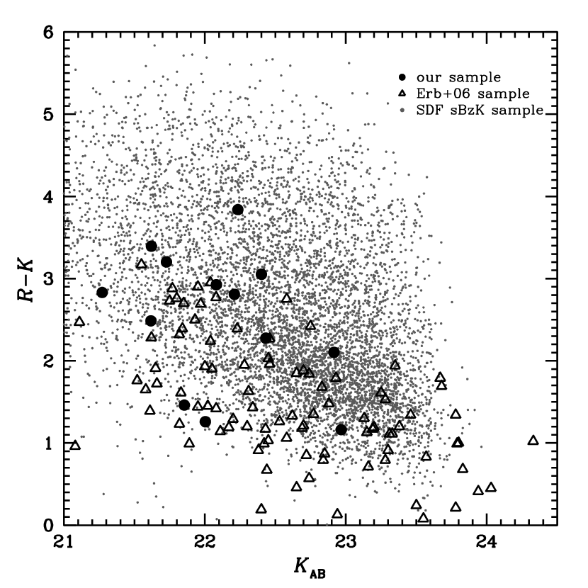
Figure 13: The color magnitude diagram of $R-K$ vs. $K$ for our sBzK spectroscopic sample (filled circles), the whole sBzK sample in the SDF (dots) and the NIRSPEC sample of Erb et al. (2006c) (open triangles).

6 Summary

We have carried out NIR spectroscopy of 44 BzK galaxies with $K_{\rm AB}\lesssim 23$ in the Subaru Deep Field with MOIRCS on the Subaru Telescope. The $zJ$ and $HK$ grism spectra cover wavelengths from 0.9 to 2.3 $\micron$ at a resolution of $R$=500. The 44 spectroscopic targets are selected from a large sample of BzKs in 180 arcmin² of the SDF. Among the 44 targets, 40 are classified as sBzKs and 4 as pBzKs. Half of the 44 targets are fainter than $K_{\rm AB}=22$. We detect ${\rm H}\alpha$ and some other emission lines in 15 sBzKs, nine of which have $K_{\rm AB}>22$.

Spectroscopic redshifts are derived from ${\rm H}\alpha$, and fluxes of emission lines are measured. Stellar mass and dust extinction are also obtained from SED-fitting to multiwavelength imaging data of $BVRi^{\prime}z^{\prime}K$. We have then obtained the following results.

The spectroscopic redshift distribution of the sBzKs does not peak at $z\sim 2$, and objects at $z<1.4$ are also selected. These lower-$z$ objects are near the selection boundary in the $BzK$ diagram. On the other hand, no $z>2$ objects are detected. This result suggests that a fraction of star forming galaxies at low redshifts can meet the sBzK criterion. However, the lack of objects at $z>2$ may be due to a flux-limited bias.

The ${\rm H}\alpha$ luminosities are converted into SFRs. It is found that sBzKs with higher stellar masses have larger SFRs. The correlation between SFR and stellar mass may be attributed to a larger amount of gas for more massive galaxies. Dividing SFR by stellar mass, specific SFRs are also derived. A negative relation is seen between stellar mass and SSFR, which is consistent with previous results for $z\sim 2$ galaxies. This negative relation implies that a proportionately larger growth of stellar mass occurs in less massive galaxies.

Gas-phase oxygen abundances, 12+log(O/H), are derived from the ratio of [N II]($\lambda 6584$) to ${\rm H}\alpha$ using the N2 index method. We have found a correlation between stellar mass and oxygen abundances, in the sense that more massive sBzKs tend to be more metal-rich, which is qualitatively consistent with the relation for UV-selected $z\sim 2$ galaxies. However, the metallicities of sBzKs are on average higher by $\sim 0.2$ dex than that of UV-selected galaxies at similar redshifts, and are close to those of local galaxies. Compared with the uncertainties, this difference in metallicity between sBzKs and UV-selected galaxies is significant, and may be due to the color difference between the two populations. Our sBzKs have redder $R-K$ colors than the UV-selected galaxies. Further, an sBzK with a blue color similar to the UV-selected galaxies has a lower abundance, comparable to those of the UV-selected galaxies. These facts suggest that there is a color-dependence in the oxygen abundance in galaxies at $z\sim 2$, which may imply that galaxies with different ages and/or dust amounts have different metallicities.

Table 1: Photometric properties of 15 sBzKs with emission lines detected.

	Magnitude	Color		SED Fitting
ID	$K$	$B-z$	$z-K$	stellar mass	$E(B-V)$
21193	21.3	1.69	1.89	3.8	0.51
21360	21.6	1.61	1.53	1.5	0.43
21667	22.1	1.24	2.15	5.5	0.38
21973	22.4	1.09	1.53	1.9	0.31
22424	22.2	1.72	2.65	15	0.45
22602	22.2	1.23	1.98	5.1	0.35
25528	22.3	1.21	1.49	1.2	0.41
26411	21.7	1.47	2.38	5.4	0.44
26821	21.8	1.10	1.24	2.1	0.38
26840	23.0	0.73	0.89	0.61	0.29
27677	22.4	1.37	2.57	3.6	0.45
27815	22.9	1.06	1.45	1.4	0.36
28761	21.9	1.04	1.02	1.5	0.35
31340	21.6	1.46	2.53	11	0.41
31569	22.0	0.78	0.74	0.61	0.23

Table 2: Spectroscopic properties of 15 sBzKs with emission lines detected.

ID	Detected Lines	redshift	$F_{{\rm H}\alpha}$	$L_{{\rm H}\alpha}$	SFRHα	EWHα	12+log(O/H)
21193	${\rm H}\alpha$,[N II]	1.479	10.9$\pm$1.77	1.5$\pm$0.24	4.2$\pm$0.68	1.8$\pm$0.56	8.78${}^{+0.08}_{-0.13}$
21360	${\rm H}\alpha$	1.174	4.16$\pm$2.25	0.32$\pm$0.18	0.49$\pm$0.27	0.86$\pm$0.53	$<$8.84
21667	${\rm H}\alpha$	1.750	11.1$\pm$2.26	2.3$\pm$0.47	2.5$\pm$0.51	4.5$\pm$1.8	$<$8.68
21973	${\rm H}\alpha$,[O III]	1.504	18.3$\pm$3.58	2.6$\pm$0.51	1.8$\pm$0.36	8.5$\pm$8.4	$<$8.75
22424	${\rm H}\alpha$,[N II]	2.018	7.25$\pm$1.24	2.1$\pm$0.37	3.9$\pm$0.66	7.0$\pm$6.9	8.80${}^{+0.07}_{-0.09}$
22602	${\rm H}\alpha$	1.872	7.72$\pm$2.35	1.9$\pm$0.58	1.7$\pm$0.52	1.1$\pm$0.46	$<$8.88
25528	${\rm H}\alpha$,[N II]	1.506	9.99$\pm$2.00	1.4$\pm$0.29	2.0$\pm$0.40	3.3$\pm$1.4	8.94${}^{+0.08}_{-0.12}$
26411	${\rm H}\alpha$,[N II]	1.498	14.0$\pm$2.67	2.0$\pm$0.38	3.3$\pm$0.63	2.7$\pm$1.2	8.70${}^{+0.12}_{-0.23}$
26821	${\rm H}\alpha$,${\rm H}\beta$,[O III],[N II]	2.044	22.2$\pm$1.43	6.8$\pm$0.44	7.3$\pm$0.47	5.9$\pm$1.2	8.66${}^{+0.06}_{-0.07}$
26840	${\rm H}\alpha$,${\rm H}\beta$,[O II],[O III],[N II]	2.012	8.98$\pm$1.37	2.6$\pm$0.40	1.5$\pm$0.23	6.6$\pm$4.6	8.52${}^{+0.09}_{-0.14}$
27677	${\rm H}\alpha$	1.710	4.53$\pm$1.39	0.89$\pm$0.27	1.6$\pm$0.50	2.8$\pm$1.6	$<$8.88
27815	${\rm H}\alpha$,[N II]	1.796	7.75$\pm$1.01	1.7$\pm$0.22	1.7$\pm$0.22	5.5$\pm$4.0	8.60${}^{+0.10}_{-0.18}$
28761	${\rm H}\alpha$,[N II]	1.818	10.3$\pm$4.90	2.3$\pm$1.1	2.1$\pm$1.0	1.8$\pm$0.91	8.68${}^{+0.19}_{-8.68}$
31340	${\rm H}\alpha$,[N II]	1.719	7.10$\pm$1.39	1.4$\pm$0.28	2.0$\pm$0.39	2.5$\pm$0.73	8.81${}^{+0.08}_{-0.13}$
31569	${\rm H}\alpha$,${\rm H}\beta$,[O III],[N II]	1.250	33.0$\pm$2.05	3.0$\pm$0.19	1.1$\pm$0.07	9.9$\pm$5.5	8.28${}^{+0.12}_{-0.25}$

References

- Alonso-Herrero et al. (2007) Alonso-Herrero, A., et al. 2008, arXiv:0712.3121
- Asplund et al. (2004) Asplund, M., Grevesse, N., Sauval, A. J., Allende Prieto, C., Kiselman, D. 2004, A&A, 417, 751
- Baldwin et al. (1981) Baldwin, J. A., Phillips, M. M., & Terlevich, R. 1981, PASP, 93, 5
- Blanc et al. (2008) Blanc, G. A., et al. 2008, arXiv:0803.0763
- Bolzonella et al. (2000) Bolzonella, M, Miralles, J. M., & Pell, R. 2000, A&A, 363, 476
- Brooks et al. (2007) Brooks, A. M., et al. 2007, ApJ, 655, L17
- Bruzual & Charlot (2003) Bruzual, A. G., & Charlot, S. 2003, MNRAS, 344, 100
- Calzetti et al. (2000) Calzetti, D., et al. 2000, ApJ, 533, 682
- Chabrier (2003) Chabrier, G. 2003, PASP, 115, 763
- Colbert et al (2005) Colbert, J. W., Teplitz, H. I., Yan, L., Malkan, M. A., McCarthy, P. J. 2005, ApJ, 621, 587
- Coleman et al. (1980) Coleman, G. D., Wu, C.-C., & Weedman, D. W. 1980, ApJS, 43, 393
- Daddi et al. (2004) Daddi, E., et al. 2004, ApJ, 617, 746
- Daddi et al. (2007) Daddi, E., et al. 2007, ApJ, 670, 156
- Daddi et al. (2008) Daddi, E., Dannerbauer, H., Elbaz, D., Dickinson, M., Morrison, G., Stern, D., & Ravindranath, S. 2008, ApJ, 673, L21
- Dannerbauer et al. (2006) Dannerbauer, H., et al. 2006, ApJ, 637, L5
- De Dossi et al. (2007) De Rossi, M. E., Tissera, P. B. & Scannapieco, C. 2007, MNRAS, 374, 323
- Dickinson et al. (2003) Dickinson, M., Papovich, C., Ferguson, H. C., & Budavri, T. 2003, ApJ, 587, 25
- Erb et al. (2006a) Erb, D. K., Shapley, A. E., Pettini., M., Steidel, C. C, Reddy, N. A., & Adelberger, K. L. 2006a, ApJ, 644, 813
- Erb et al. (2006b) Erb, D. K., Steidel, C. C, Shapley, A. E., Pettini., M., Reddy, N. A., & Adelberger, K. L. 2006b, ApJ, 647, 128
- Erb et al. (2006c) Erb, D. K., Steidel, C. C, Shapley, A. E., Pettini., M., Reddy, N. A., & Adelberger, K. L. 2006c, ApJ, 646, 107
- Gallazzi et al. (2005) Gallazzi, A., Chrlot, S., Brinchmann, J., White, S. D. M., & Tremonti, C. A. 2005, MNRAS, 362, 41
- Grazian et al. (2007) Grazian, A., et al. 2007, A&A, 465, 393
- Finlator & Dav (2008) Finlator, K. & Dav, R. 2008, MNRAS, 385, 2181
- Fontana et al. (2003) Fontana, A., et al. 2003, ApJ, 594, L9
- Halliday et al. (2008) Halliday, C., et al. 2008, arXiv:0801.1193
- Hayashi et al. (2007) Hayashi, M., Shimasaku, K., Motohara, K., Yoshida, M., Okamura S. & Kashikawa, N. 2007, ApJ, 660, 72
- Hicks et al. (2002) Hicks, E. K., Malkan, M. A., Teplitz, H. I., McCarthy, P. J., and Yan, L. 2002, ApJ, 581, 205
- Ichikawa et al. (2006) Ichikawa, T., et al. 2006 Proc. SPIE, 6269, 38
- Kajisawa & Yamada (2001) Kajisawa, M., & Yamada, T. 2001, PASJ, 53, 833
- Kashikawa et al. (2004) Kashikawa, N., et al. 2004, PASJ, 56, 1011
- Kauffmann et al. (2003) Kauffmann, G., et al. 2003, MNRAS, 346, 1055
- Kennicutt (1998) Kennicutt, R. C. 1998, ARA&A, 36, 189
- Kewley & Dopita (2002) Kewley, L. J. & Dopita, M. A. 2002, ApJS, 142, 35
- Kobulnicky & Kewley (2004) Kobulnicky, H. A. & Kewley, L. J. 2002, ApJ, 617, 240
- Kriek et al. (2008) Kriek, M., et al. 2008, arXiv:0801.1110
- Kong et al. (2006) Kong, X., et al. 2006, ApJ, 638, 72
- Lane et al. (2007) Lane, K. P., et al. 2007, MNRAS, 379, L25
- Liu et al. (2008) Liu, X., Shapley, A. E., Coil, A. L., Brinchmann, J. & Ma, C. P. 2008, ApJ, 678, 758
- Ly et al. (2008) Ly, C. et al. 2008, in preparation
- Ly et al. (2007) Ly, C. et al., 2007, ApJ, 657, 738
- Maiolino et al. (2008) Maiolino, R., et al. 2008, A&A, 488, 463
- Malkan & Filippenko (1983) Malkan, A. M., & Filippenko, A. V. 1983, ApJ, 275, 477
- McCarthy et al. (1999) McCarthy, P. J. et al., 1999, ApJ, 520, 548
- Peng et al. (2002) Peng, C. Y., Ho, L. C., Impey, C. D. & Pix, H.-W. 2002 AJ, 124, 266
- Pettini & Pagel (2004) Pettini, M. & Pagel, B. E. J. 2004 MNRAS, 348, L59
- Pickles (1998) Pickles, A. J. 1998, PASP, 110, 863
- Press et al. (1995) Press, W. H., et al. 1995, Numerical recipes (Cambridge: Cambridge University Press)
- Reddy et al. (2006a) Reddy, N. A., et al. 2006a ApJ, 644, 792
- Reddy et al. (2006b) Reddy, N. A., Steidel, C. C., Erb, D. K., Shapley, A. E., & Pettini, M. 2006b ApJ, 653, 1004
- Richards et al. (2006) Richards, G. T., et al. 2006, AJ, 131, 2766
- Salpeter (1955) Salpeter, E. E. 1955, ApJ, 121, 161
- Savaglio et al. (2005) Savaglio, S., et al. 2005, ApJ, 635, 260
- Sawicki (2002) Sawicki, M. 2002, AJ, 124, 3050
- Spinoglio et al. (1995) Spinoglio, L., Malkan, M. A., Rush, B., Carrasco, L. & Recillas-Cruz, E. 1995, ApJ, 453, 616
- Storchi-Bergmann et al. (1994) Storchi-Bergmann, T., Calzetti, D., & Kinney, A. L. 1994, ApJ, 429, 572
- Takagi et al. (2003) Takagi, T., Arimoto, N. & Hanami, H. 2003, MNRAS, 340, 813
- Tremonti et al. (2004) Tremonti, C. A., et al. 2004, ApJ, 613, 898
- Veilleux & Osterbrock (1987) Veilleux S. & Osterbrock D. E. 1987, ApJS, 63, 295