Application of a Self-Similar Pressure Profile to Sunyaev-Zel’dovich Effect Data from Galaxy Clusters

Abstract

We investigate the utility of a new, self-similar pressure profile for fitting Sunyaev-Zel’dovich (SZ) effect observations of galaxy clusters. Current SZ imaging instruments—such as the Sunyaev-Zel’dovich Array (SZA)—are capable of probing clusters over a large range in physical scale. A model is therefore required that can accurately describe a cluster’s pressure profile over a broad range of radii, from the core of the cluster out to a significant fraction of the virial radius. In the analysis presented here, we fit a radial pressure profile derived from simulations and detailed X-ray analysis of relaxed clusters to SZA observations of three clusters with exceptionally high quality X-ray data: A1835, A1914, and CL J1226.9+3332. From the joint analysis of the SZ and X-ray data, we derive physical properties such as gas mass, total mass, gas fraction and the intrinsic, integrated Compton $y$-parameter. We find that parameters derived from the joint fit to the SZ and X-ray data agree well with a detailed, independent X-ray-only analysis of the same clusters. In particular, we find that, when combined with X-ray imaging data, this new pressure profile yields an independent electron radial temperature profile that is in good agreement with spectroscopic X-ray measurements.

1 Introduction

The expansion history of the universe and the growth of large-scale structure are two of the most compelling topics in cosmology. As galaxy clusters are the largest collapsed objects in the universe, taking a Hubble time to form, their abundance and evolution are critically sensitive to the details of that expansion history. Cluster surveys can therefore provide fundamental clues to the nature and abundance of dark matter and dark energy (see, e.g., White et al., 1993; Frenk et al., 1999; Haiman et al., 2001; Weller et al., 2002).

While clusters have been extensively studied using X-ray observations of the hot gas that comprises the intracluster medium (ICM), radio measurements of the same gas via the Sunyaev-Zel’dovich (SZ) effect (Sunyaev & Zel’dovich, 1972) provide an independent and complementary probe of the ICM (e.g., Carlstrom et al., 2002). The SZ effect arises from inverse Compton scattering of cosmic microwave background (CMB) photons by the electrons in the ICM, imparting a detectable spectral signature to the CMB that is independent of the redshift of the cluster. As the SZ effect is a measure of the integrated line-of-sight electron density, weighted by temperature, i.e., the integrated pressure (see § 2.1), it probes different properties than the X-ray emission, which is proportional to the square of the electron density. Cluster surveys exploiting the redshift independence of the SZ effect are now being conducted by a variety of instruments, including the SZA (Muchovej et al., 2007), the South Pole Telescope (Ruhl et al., 2004), the Atacama Cosmology Telescope (Kosowsky, 2003) and the Atacama Pathfinder Experiment (APEX) SZ instrument (Dobbs et al., 2006).

To maximize the utility of clusters as cosmological probes we must understand how to accurately relate their observable properties to their total masses. The integrated SZ signal from a cluster is proportional to the total thermal energy of the cluster, and is therefore a measure of the underlying gravitational potential, and ultimately the dark matter content, within a cluster. The SZ flux of a cluster thereby should provide a robust, low scatter proxy for the total cluster mass, $M_{\mbox{\scriptsize tot}}$ (see, for example, da Silva et al., 2004; Motl et al., 2005; Nagai, 2006; Reid & Spergel, 2006).

To date, cosmological studies combining SZA and X-ray data have relied almost exclusively on the isothermal $\beta$-model (first used in Cavaliere & Fusco-Femiano, 1976, 1978) to fit the SZ signal in the region interior to $r_{2500}$ (see Grego et al., 2000; Reese et al., 2002; LaRoque et al., 2006; Bonamente et al., 2006, 2008, for applications of the isothermal $\beta$-model to SZ+X-ray data). Here $r_{2500}$ is the radius within which the mean cluster density is a factor of 2500 over the critical density of the universe at the cluster redshift. While the isothermal $\beta$-model recovers global properties of clusters quite accurately in this regime (LaRoque et al., 2006), deep X-ray observations of nearby clusters show that isothermality is a poor description of the cluster outskirts ($r\sim r_{500}$) (see e.g. Piffaretti et al., 2005; Vikhlinin et al., 2005; Pratt et al., 2007, and references therein). An improved model for the cluster gas, accurate to large radii, is therefore critical for the analysis and cosmological interpretation of SZ data obtained with new instruments that are capable of probing the outer regions ($r\sim r_{500}$) of clusters. Such a model must be simple enough that it can be constrained by SZ data with limited angular resolution and sensitivity typical of data sets acquired by SZ survey instruments optimized for detection, rather than imaging. While the $\beta$-model has the virtue of simplicity, previous attempts to relax the assumption of isothermality typically required high-significance, spatially-resolved X-ray spectroscopy; such data are seldom obtained in short X-ray exposures of high-redshift clusters. This is particularly true for the cluster outskirts (see, e.g., LaRoque et al., 2006). Attempts to move beyond the $\beta$-model have typically improved the modeling of the gas density only within the core ($r\lesssim 0.15\,r_{500}$).

In this work, we investigate a new model for the cluster gas pressure by using it to fit SZ data from the SZA and X-ray data from Chandra to three well-studied clusters: Abell 1835, Abell 1914, and CL J1226.9+3332. The model was derived by Nagai et al. (2007) from simulations and from detailed analysis of deep Chandra measurements of nearby relaxed clusters. The simplicity of this model—and the fact that SZ data are inherently sensitive to the integrated electron pressure—allow it to be used either in conjunction with X-ray imaging data, or fit to SZ data alone. The outline of the paper is as follows: in § 2, we present the details of the model, and couple it with an ICM density model that allows the inclusion of X-ray imaging data. In § 3, we apply this method to three clusters, combining new data from the SZA with Chandra X-ray imaging data. We demonstrate the utility of this model by applying it to SZ+X-ray data without relying on X-ray spectroscopic information. Results from the joint SZ+X-ray analysis are then compared to results from an X-ray-only analysis, including spectroscopic data, in § 4. We offer our conclusions in § 5.

2 Cluster Gas Models

2.1 Sunyaev Zel’dovich Effect and X-ray Emission

The thermal SZ effect is a small ($<10^{-3}$) distortion in CMB intensity caused by inverse Compton scattering of CMB photons by energetic electrons in the hot intracluster gas (Sunyaev & Zel’dovich, 1970, 1972). This spectral distortion can be expressed, for dimensionless frequency $x\equiv h\nu/\mbox{$k_{\mbox{\tiny B}}$}\mbox{$T_{\mbox{\tiny CMB}}$}$, where $h$ is Planck’s constant, $\nu$ is frequency, $k_{B}$ is Boltzmann’s constant, and $T_{\mbox{\tiny CMB}}$ is the primary CMB temperature, as the change $\Delta I_{SZ}$ relative to the primary CMB intensity normalization $I_{0}$,

$$\frac{\Delta I_{SZ}}{I_{0}} = \frac{k_{B}\,\sigma_{T}}{m_{e}c^{2}}\int\!\!g(x,T_{e})\,n_{e}T_{e}\,d\ell$$ (1)

$$= \frac{\sigma_{T}}{m_{e}c^{2}}\int\!\!g(x,T_{e})\,P_{e}\,d\ell.$$ (2)

Here $\sigma_{\mbox{\tiny T}}$ is the Thomson scattering cross-section of the electron, $\ell$ is the line of sight, and $m_{e}c^{2}$ is an electron’s rest energy. The factor $g(x,T_{e})$ encapsulates the frequency dependence of the SZ effect intensity. For non-relativistic electrons,

$$g(x)=\frac{x^{4}e^{x}}{(e^{x}-1)^{2}}\left(x\frac{e^{x}+1}{e^{x}-1}-4\right).$$ (3)

We use the Itoh et al. (1998) relativistic corrections to Eq. 3, which are appropriate for fitting thermal SZ observations, and discuss their impact on the fit ICM profiles in § 4.3. Note that we have used the ideal gas law ($P_{e}=n_{e}k_{B}T_{e}$) to obtain Eq. 2 from Eq. 1; we use this to relate SZ intensity directly to the ICM electron pressure.

The X-ray emission from massive clusters arises predominantly as thermal bremsstrahlung from electrons. The X-ray surface brightness produced by a cluster at redshift $z$ is given by (e.g., Sarazin, 1988)

$$S_{X}=\frac{1}{4\pi(1+z)^{4}}\!\int\!\!n_{e}^{2}\mbox{$\Lambda_{ee}$}(T_{e},Z)\,d\ell,$$ (4)

where the integral is evaluated along the line of sight and the X-ray cooling function $\Lambda_{ee}$ is proportional to $T_{e}^{1/2}$. The X-ray emission is therefore proportional to the square of the gas density, with a relatively weak dependence on $T_{e}$. Separate spectroscopic observations of X-ray line emission can be used to measure the gas temperature. Throughout this work, we use the Raymond-Smith plasma emissivity code (Raymond & Smith, 1977) with constant metallicity $Z=0.3Z_{\odot}$, yielding $\mu_{e}=1.17$ and $\mu=0.61$ for the mean molecular weight of the electrons and gas, respectively, using the elemental abundances provided by Anders & Grevesse (1989). The SZ and X-ray observables $\Delta I_{SZ}$ and $S_{X}$ are computed by evaluating the integrals in Eqs. 2 & 4 numerically.

2.2 Three-dimensional Models of the ICM Profiles

In this work, we adopt an analytic parameterization of the cluster radial pressure profile proposed by Nagai et al. (2007) (hereafter N07),

$$P_{e}(r)=\frac{P_{e,i}}{(r/r_{p})^{c}\left[1+(r/r_{p})^{a}\right]^{(b-c)/a}},$$ (5)

where $P_{e,i}$ is a scalar normalization of the pressure profile, $r_{p}$ is a scale radius (typically $r_{p}\approx r_{500}/1.3$), and the parameters $(a,b,c)$ respectively describe the slopes at intermediate ($r\approx r_{p}$), outer ($r>r_{p}$), and inner ($r\ll r_{p}$) radii. Note that Eq. 5 is a generalization of the analytic fitting formula obtained in numerical simulations as a parameterization of the distribution of mass in a dark matter halo (Navarro et al., 1997, NFW profile). This choice is reasonable because the gas pressure distribution is primarily determined by the dark matter potential. The use of a parameterized pressure profile is further motivated by the fact that self-similarity is best preserved for pressure, as demonstrated by the low cluster-to-cluster scatter seen when using these parameters to fit numerical simulations. The NFW profile – in its pure form – has been applied by Atrio-Barandela et al. (2008) to fit the electron pressure profiles of SZ observations of clusters, who demonstrated an improvement over the application of the isothermal $\beta$-model to SZ cluster studies. In this work, we adopt the fixed slopes $(a,b,c)=(0.9,5.0,0.4)$, which N07 found to closely match the observed profiles of the Chandra X-ray clusters and the results of numerical simulations in the outskirts of a broad range of relaxed clusters.

The density model used to fit the X-ray image data is a simplified version of the model employed by Vikhlinin et al. (2006) (hereafter V06) is

$$n_{e}^{2}(r)=n_{e0}^{2}\;\frac{(r/r_{c})^{-\alpha}}{\left[1+(r/r_{c})^{2}\right]^{3\beta-\alpha/2}}\\ \frac{1}{\left[1+(r/r_{s})^{\gamma}\right]^{\varepsilon/\gamma}}\\ +\frac{n_{e02}^{2}}{\left[1+(r/r_{c2})^{2}\right]^{3\beta_{2}}}.$$ (6)

We refer to Eq. 6, used in the independent X-ray analysis to which we compare our SZ+X-ray results, as the “V06 density model.” Since the cluster core contributes negligibly to the SZ signal observed by the SZA, we exclude the inner 100 kpc of the cluster from the X-ray images used in the joint SZ+X-ray analysis. Recognizing as the component introduced by Pratt & Arnaud (2002) to fit the inner slope of a cuspy cluster density profile, and that the second $\beta$-model component ($\beta_{2}$) is present explicitly to fit the cluster core, we simplify the V06 density model to

$$n_{e}(r)=n_{e0}\left[1+(r/r_{c})^{2}\right]^{-3\beta/2}\left[1+(r/r_{s})^{\gamma}\right]^{-0.5\varepsilon/\gamma},$$ (7)

where $r_{c}$ is the core radius, and $r_{s}$ is the radius at which the density profile steepens with respect to the traditional $\beta$-model. Following V06, we fix $\gamma=3$, as this provides an adequate fit to all clusters in the V06 sample. We refer to this model as the “Simplified Vikhlinin Model” (SVM). Note that in the limit $\varepsilon\rightarrow 0$, Eq. 7 reduces to the standard $\beta$-model. The SVM is thus a modification to the $\beta$-model that has the additional freedom to extend from the core ($r\gtrsim r_{c}$) to the outer regions of cluster gas, spanning intermediate ($r\gtrsim r_{s}$) to large radii ($r\sim r_{500}$).

With the electron pressure and density in hand, we may also derive the electron temperature of the ICM using the ideal gas law, $T_{e}(r)=P_{e}(r)/k_{B}n_{e}(r)$, where $P_{e}$ and $n_{e}$ are given by Eqs. 5 and 7, respectively. Note that $T_{e}(r)$ derived in this way is used in the analysis of X-ray surface brightness (Eq. 4). Hereafter, we refer to this jointly-fit cluster gas model as the N07+SVM profile.

For comparison with previous work (e.g. Bonamente et al., 2008), we also employ the isothermal $\beta$-model for joint analysis of the SZ and X-ray data. In this model the density is given by Eq. 7 with $\varepsilon=0$ and $T_{e}(r)$ is a constant equal to the spectroscopically-measured temperature, $T_{X}$. The shape parameters of the isothermal $\beta$-model, $r_{c}$ and $\beta$, are jointly fit to the SZ and X-ray data, while the X-ray surface brightness (Eq. 4) and SZ intensity profile (Eq. 2) normalizations are independently determined from the X-ray and SZ data, respectively.

2.3 Parameter Estimation Using the Markov Chain Monte Carlo Method

Our models have five free parameters to describe the radial distribution of the gas density (see Eq. 7) and two parameters for the electron pressure (see Eq. 5). Additional parameters such as the cluster centroid, X-ray background level, as well as the positions, fluxes and spectral indices of compact radio sources are also included where necessary. The Markov chain Monte Carlo (MCMC) method is used to extract the model parameters from the SZ and X-ray data, as described by Bonamente et al. (2004). In this section we provide a brief overview of this method, focusing on the changes to accommodate the N07 pressure model.

The first step in fitting the SZ data is to compute the model image over a regular grid, sampled at less than half the smallest scale the SZA can probe. This image is multiplied by the primary beam of the SZA, transformed via FFT to Fourier space (where the data are naturally sampled by an interferometer; see § 4.1), and interpolated to the Fourier-space coordinates of the SZ data. The likelihood function for the SZ data is then computed directly in the Fourier plane, where the noise properties of the interferometric data are well-characterized.

The first step of the MCMC method is the calculation of the joint likelihood $\mathcal{L}$ of the X-ray and SZ data with the model. The SZ likelihood is given by

$$\ln(\mathcal{L}_{SZ})=\displaystyle\sum_{i}\left[-\frac{1}{2}\left(\Delta R_{i}^{2}+\Delta I_{i}^{2}\right)\right]W_{i},$$ (8)

where $\Delta R_{i}$ and $\Delta I_{i}$ are the differences between model and data for the real and imaginary components at each point $i$ in the Fourier plane, and $W_{i}$ is a measure of the Gaussian noise ($1/\sigma^{2}$).

Since the X-ray counts, treated in image space, are distributed according to Poisson statistics, the likelihood of the model fit is given by

$$\ln(\mathcal{L}_{image})=\displaystyle\sum_{i}\left[D_{i}\ln(M_{i})-M_{i}-\ln(D_{i}!)\right],$$ (9)

where $M_{i}$ is the model prediction (including cluster and background components), and $D_{i}$ is the number of counts detected in pixel $i$. The inner 100 kpc of the X-ray images—as well as any detected X-ray point sources—are excluded from the fits by excluding these regions from the calculation of $\ln(\mathcal{L}_{image})$ in Eq. 9.

The joint likelihood of the spatial and spectral models is given by $\mathcal{L}=\mathcal{L}_{SZ}\mathcal{L}_{Xray}$. For the N07+SVM fits, $\mathcal{L}_{Xray}$ is simply $\mathcal{L}_{image}$. Following Bonamente et al. (2004, 2006), the X-ray likelihood for the $\beta$-model fits is $\mathcal{L}_{image}\mathcal{L}_{Xspec}$, as these must incorporate the likelihood $\mathcal{L}_{Xspec}$ of the spectroscopic determination of $T_{X}$. The likelihood is used to generate the Markov parameter chains, and convergence of the chain to a stationary distribution is established using the Raftery-Lewis and Geweke tests (Raftery & Lewis, 1992; Gilks et al., 1996).

2.4 Calculation of $M_{\mbox{\scriptsize gas}}$, $M_{\mbox{\scriptsize tot}}$, and $Y_{\mbox{\scriptsize int}}$

With knowledge of the three-dimensional gas profiles, we compute global properties of galaxy clusters as follows. The gas mass $\mbox{$M_{\mbox{\scriptsize gas}}$}(r)$ enclosed within radius $r$ is obtained by integrating the gas density $\mbox{$\rho_{\mbox{\scriptsize gas}}$}\equiv\mu_{e}m_{p}n_{e}(r)$ over a spherical volume:

$$\mbox{$M_{\mbox{\scriptsize gas}}$}(r)=4\pi\!\int_{0}^{r}\!\mbox{$\rho_{\mbox{\scriptsize gas}}$}(r^{\prime})r^{\prime 2}dr^{\prime}.$$ (10)

The total mass, $M_{\mbox{\scriptsize tot}}$, can be obtained by solving the hydrostatic equilibrium equation as:

$$\mbox{$M_{\mbox{\scriptsize tot}}$}(r)=-\frac{r^{2}}{G\mbox{$\rho_{\mbox{\scriptsize gas}}$}(r)}\frac{dP(r)}{dr},$$ (11)

where $P=(\mu_{e}/\mu)P_{e}$ is the total gas pressure. We then compute the gas mass fractions as $\mbox{$f_{\mbox{\scriptsize gas}}$}=\mbox{$M_{\mbox{\scriptsize gas}}$}/\mbox{$M_{\mbox{\scriptsize tot}}$}$.

The line of sight Compton $y$-parameter, which characterizes the strength of Compton scattering by electrons, is defined

$$y\equiv\frac{k_{B}\sigma_{T}}{m_{e}c^{2}}\int\!\!n_{e}T_{e}\,d\ell.$$ (12)

We compute the volume-integrated Compton $y$-parameter, $Y$, from the pressure profile fit to the SZ observations for both cylindrical and spherical volumes of integration. The cylindrically-integrated quantity, $Y_{\mbox{\scriptsize cyl}}$, is calculated within an angle $\theta$ on the sky, corresponding to physical radius $R=\theta d_{A}$ at the redshift of the cluster,

$$\mbox{$Y_{\mbox{\scriptsize cyl}}$}\left(R\right)\equiv 2\pi\,{d_{A}^{2}}\int_{0}^{\theta}\!\!y\left(\theta\right)\,\theta^{\prime}d\theta^{\prime}=2\pi\int_{0}^{R}\!\!y\left(r^{\prime}\right)\,r^{\prime}dr^{\prime}=\frac{2\pi\,\sigma_{T}}{m_{e}\,c^{2}}\int_{-\infty}^{\infty}\!\!d\ell\int_{0}^{R}\!P_{e}\left(r^{\prime}\right)\,r^{\prime}dr^{\prime}.$$ (13)

The last form makes explicit the infinite limits of integration in the line of sight direction, originating with the definition of $y$ (Eqs. 1 and 2). The spherically-integrated quantity, $Y_{\mbox{\scriptsize sph}}$, is obtained by integrating the pressure profile within a radius $r$ from the cluster center,

$$\mbox{$Y_{\mbox{\scriptsize sph}}$}(r)=\frac{4\pi\,\sigma_{T}}{m_{e}\,c^{2}}\int_{0}^{r}\!\!P_{e}(r^{\prime})\,r^{\prime 2}dr.$$ (14)

The parameter $\mbox{$Y_{\mbox{\scriptsize sph}}$}(r)$ is thus proportional to the thermal energy content of the ICM.

To compute the global cluster properties described above, one needs to define a radius out to which all quantities will be calculated. Following LaRoque et al. (2006) and Bonamente et al. (2006), we compute global properties of clusters enclosed within the overdensity radius $r_{\Delta}$, within which the average density $\langle\rho\rangle$ of the cluster is a specified fraction $\Delta$ of the critical density, via

$$\frac{4}{3}\pi\,\rho_{c}(z)\,\Delta\,r_{\Delta}^{3}=\mbox{$M_{\mbox{\scriptsize tot}}$}(r_{\Delta}),$$ (15)

where $\rho_{c}(z)$ is the critical density at cluster redshift $z$, and $\Delta\equiv\langle\rho\rangle/\rho_{c}(z)$. In this work, we evaluate cluster properties at density contrasts of $\Delta=2500$ and $\Delta=500$. The overdensity radius $r_{2500}$ has been used in previous OVRO and BIMA interferometric SZ studies (e.g. LaRoque et al., 2006; Bonamente et al., 2008) as well as in many X-ray cluster studies (e.g. Vikhlinin et al., 2006; Allen et al., 2007), while $r_{500}$ is a radius reachable with SZA and deep Chandra X-ray data.

3 Data

3.1 Cluster Sample

For this work, we selected three massive clusters that are well studied at X-ray wavelengths, and span a range of redshifts ($z$ = 0.17–0.89) and morphologies, on which to test the joint analysis of the Chandra X-ray and SZA data. We assume a $\Lambda$CDM cosmology with $\Omega_{M}=0.3$, $\Omega_{\Lambda}=0.7$, and $h=0.7$ throughout our analysis.

Located at $z=0.25$, Abell 1835 (A1835) is an intermediate-redshift, relaxed cluster, as evidenced by its circular morphology in the X-ray images and its cooling core (Peterson et al., 2001). To demonstrate the applicability of our technique for high redshift clusters, we analyzed CL J1226.9+3332 (CL1226), an apparently relaxed cluster at $z=0.89$ (Maughan et al., 2004, 2007). To assess how this method performs on somewhat disturbed clusters, we also analyzed Abell 1914 (A1914), an intermediate redshift ($z=0.17$) cluster with a hot subclump near the core. When the subclump is not excluded from the X-ray analysis, Maughan et al. (2008, hereafter M08) find a large X-ray centroid shift in the density profile, which they use as an indicator of an unrelaxed dynamical state.

In the following sections, we discuss the instruments, data reduction, and analysis of the SZ and X-ray data. Details of these observations, including the X-ray fitting regions, the unflagged, on-source integration times, and the pointing centers used for the SZ observations, are presented in Tables 1 and 2. We also review an independent, detailed X-ray-only analysis, with which we compare the results of our joint SZ+X-ray analyses.

3.2 Sunyaev-Zel’dovich Array Observations

The Sunyaev-Zel’dovich Array is an interferometric array comprising eight 3.5-meter telescopes, and is located at the Owens Valley Radio Observatory. For the observations presented here, the instrument was configured to operate in an 8-GHz-wide band covering 27–35 GHz using the 26–36 GHz receivers (hereafter referred to as the “30-GHz” band) or covering 90–98 GHz using the 80–115 GHz receivers (the “90-GHz” band). See Muchovej et al. (2007) and Marrone et al. (in preparation) respectively for more details about commissioning observations performed with the 30-GHz and the 90-GHz SZA instruments. Details of the observations presented here, including the sensitivity and effective resolution (the synthesized beam) of the long and short baselines, are given in Table 1.

An interferometer directly measures the amplitude and phase of Fourier modes of the sky intensity, with sensitivity to a range of angular scales on the sky given by $\sim\lambda/B$, where $B$ is the projected separation of any pair of telescopes, i.e., a baseline. The field of view of the SZA is given by the primary beam of a single telescope, approximately 10.7′ at the center of the 30-GHz band. At 30 GHz, optimal detection of the arcminute-scale bulk SZ signal from clusters requires the short baselines of a close-packed array configuration; six of the SZA telescopes were arranged in this configuration for the observations presented here, yielding 15 baselines with sensitivity to $\sim$ 1–5′ scales. The two outer antennas, identical to the inner six, provide an additional 13 long baselines in this configuration, with sensitivity to small-scale structure, allowing simultaneous measurement of compact radio sources unresolved by the long baselines (angular size $\lesssim 20\arcsec$) which could otherwise contaminate the SZ signal. Observations at 90 GHz with the SZA probe scales at three times the resolution of the 30-GHz observations for the same array configuration. The short baselines of the 90-GHz observations thereby bridge the gap between long and short baseline coverage at 30-GHz.

SZA data are processed in a complete pipeline for the reduction and calibration of interferometric data, developed within the SZA collaboration. Absolute flux calibrations are derived from observations of Mars, scaled to the predictions of Rudy (1987). Data from each observation are bandpass-calibrated using a bright, unresolved, flat-spectrum radio source, observed at the start or end of an observation. The data are regularly phase-calibrated using radio sources near the targeted field; these calibrators are also used to track small variations in the antenna gains. Data are flagged for corruption due to bad weather, sources of radio interference and other instrumental effects that could impact data quality. A more detailed account of the SZA data reduction pipeline is presented in Muchovej et al. (2007).

In the SZA cluster observations presented here, the A1835 field contains three detectable compact sources at 31 GHz: a $2.8\pm 0.3$ mJy central source, a $1.1\pm 0.4$ mJy source about one arcminute from the cluster center, and a $0.8\pm 0.4$ mJy source 5.5 arcminutes from center. The positions of these sources are in good agreement with those from the NVSS (which only contains the central source) and the FIRST surveys. The SZA observation of CL1226 contains one detectable compact source, identified in both FIRST and NVSS, with flux at 31 GHz of $3.9\pm 0.2$ mJy. This source is 4.3 arcminutes from the cluster center (see also Muchovej et al., 2007) and therefore lies outside the field of view of the SZA 90 GHz observations. Two compact sources, with positions constrained by NVSS and FIRST, were detected at 31 GHz in the A1914 field. The fluxes of these sources are $1.8\pm 0.4$ mJy and $1.2\pm 0.3$ mJy. The stronger was detected in both the NVSS and the FIRST surveys, while the weaker was only detected in the FIRST survey. Table 3 summarizes the properties of the compact radio sources detected in the SZA observations.

When fitting compact sources detected in the SZ observations, we calculated the spectral indices from the measured flux at 31 GHz and 1.4 GHz, where the latter was constrained by either the NVSS (Condon et al., 1998) or FIRST (White et al., 1997) survey, respectively. The source fluxes and approximate coordinates are first identified using the interferometric imaging package Difmap (Shepherd, 1997). We first refine the source positions by fitting a model in the MCMC routine, and then fix these positions to their best-fit values when fitting the cluster SZ model. We leave the source flux a free parameter, so that the cluster SZ flux and any compact sources are fit simultaneously.

3.3 X-ray Observations

All X-ray imaging data used in this analysis were obtained with the Chandra ACIS-I detector, which provides spatially resolved X-ray spectroscopy and imaging with an angular resolution of $\sim 0.5\arcsec$ and energy resolution of $\sim$ 100–200 eV. Table 2 summarizes the X-ray observations of individual clusters.

For the X-ray data used in the joint SZ+X-ray analysis, images were limited to 0.7–7 keV in order to exclude the data most strongly affected by background and by calibration uncertainties. The X-ray images—which primarily constrain the ICM density profiles—were binned in 1.97$\arcsec$ pixels; this binning sets the limiting angular resolution of our processed X-ray data, as the Chandra point response function in the center of the X-ray image is smaller than our adopted pixel size. The X-ray background was measured for each cluster exposure, using source-free, peripheral regions of the adjacent detector ACIS-I chips. Additional details of the Chandra X-ray data analysis are presented in Bonamente et al. (2004, 2006).

In § 4.3 & 4.4 we compare the results of our joint SZ+X-ray analysis to the results of independent X-ray analyses. For A1914 and CL1226 we use the data and analysis described in detail in M08 and Maughan et al. (2007) (hereafter M07), respectively. For A1835, the ACIS-I observations used became public after the M08 sample was published, and we therefore present its analysis here for the first time. The observation of A1835 was calibrated and analyzed using the same methods and routines described in M08, which we now briefly review.

In the X-ray-only analyses, blank-sky fields are used to estimate the background for both the imaging and spectral analysis. The imaging analysis (primarily used to obtain the gas emissivity profile) is performed in the 0.7–2 keV energy band to maximize signal to noise. Similar to the joint SZ+X-ray analyses, these images were also binned into 1.97$\arcsec$ pixels.

For the spectral analysis, spectra extracted from a region of interest were fit in the 0.6–9 keV band with an absorbed, redshifted Astrophysical Plasma Emission Code (APEC) (Smith et al., 2001) model. This absorption was fixed at the Galactic value. This spectral analysis was used to derive both the global temperature $T_{X}$, determined within the annulus $r\in[0.15,1.0]\,r_{500}$, and the radial temperature profile fits of the V06 temperature profile, given by

$$T_{\mathrm{3D}}(r)=T_{0}\left[\frac{(r/r_{\text{cool}})^{a_{\text{cool}}}+T_{\text{min}}/T_{0}}{(r/r_{\text{cool}})^{a_{\text{cool}}}+1}\right]\left[\frac{(r/r_{t})^{-a}}{(1+(r/r_{t})^{b})^{c/b}}\right].$$ (16)

We refer the reader to V06 for details, but note that this temperature profile is the combination of a cool core component (first set of square brackets, where the core temperature declines to $T_{\text{min}}$) and a decline at large radii (second set of square brackets, where temperature falls at $r\gtrsim r_{t}$).

An important consideration when using a blank-sky background method is that the count rate at soft energies can be significantly different in the blank-sky fields than in the target field, due to differences between the level of the soft Galactic foreground emission in the target field and that in the blank-sky field. This was accounted for in the imaging analysis by normalizing the background image to the count rate in the target image in regions far from the cluster center. In the spectral analysis, this was modeled by an additional thermal component that was fit to a soft residual spectrum (the difference between spectra extracted in source free regions of the target and background datasets; see Vikhlinin et al. (2005)). The exception to this was the XMM-Newton data used in addition to the Chandra data for CL1226. As discussed in M07, a local background was found to be more reliable for the spectral analysis in this case, thus requiring no correction for the soft Galactic foreground.

The M07/M08 X-ray analysis methods exploit the full V06 density and temperature models (Eqs. 6 & 16, respectively) to fit the emissivity and temperature profiles derived for each cluster, and the results of these fits are used to derive the total hydrostatic mass profiles of each system. Uncertainties for the independent, X-ray-only analysis method are derived using a Monte Carlo randomization process. These fits involved typically $\sim$1000 realizations of the temperature and surface brightness profiles, fit to data randomized according to the measured noise. We refer the reader to M07 and M08, where this fitting procedure is described in detail.

4 Results

4.1 SZ Cluster Visibility Fits

Interferometric SZ data are in the form of visibilities $V_{\nu}(u,v)$ (see, for example, Thompson et al., 2001), which for single, targeted cluster observations with the SZA can be expressed in the small angle approximation as

$$V_{\nu}(u,v)=\int\!\int A_{\nu}(x,y)\,I_{\nu}(x,y)\,{e^{-i2\pi(ux+vy)}}\,dx\,dy.$$ (17)

Here $u$ and $v$ (in number of wavelengths) are the Fourier conjugates of the direction cosines $x$ and $y$ (relative to the observing direction), $A_{\nu}(x,y)$ is the angular power sensitivity pattern of each antenna at frequency $\nu$, and $I_{\nu}(x,y)$ is the intensity pattern of the sky (also at $\nu$). Eq. 17 is recognizable as a 2-D Fourier transform, so the visibilities give the flux for the Fourier mode for the corresponding $u,v$-coordinate.

By combining Eqs. 1 and 17, we can remove the frequency dependence from the measured cluster visibilities, just as we have related SZ intensity to the frequency-independent Compton $y$-parameter. We define the frequency-independent cluster visibilities $Y(u,v)$ as

$$V_{\nu}(u,v)\equiv g(x)\,I_{0}\,Y(u,v),$$ (18)

where $I_{0}$ (in units of flux per solid angle) is

$$I_{0}=\frac{2(k_{B}\mbox{$T_{\mbox{\tiny CMB}}$})^{3}}{(hc)^{2}}.$$ (19)

Additionally, we rescale $Y(u,v)$ by the square of the angular diameter distance, $d_{A}^{2}$, in order to remove the redshift dependence from the cluster SZ signal. Note that, while we use the non-relativistic $g(x)$ (Eq. 3) to compute $Y(u,v)$ (Eq. 18) , we only use this for display purposes. The effects of assuming the classical SZ frequency dependence are discussed in § 4.3.

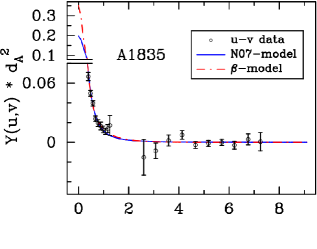
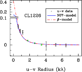
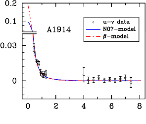
Figure 1: SZ profiles for A1835 (left), CL1226 (middle), and A1914 (right), plotted as a function of u,v-radius ($\sqrt{u^{2}+v^{2}}$). The panels show the real component of the visibilities over the full range of the fit models, using a broken axis to capture the model predictions as the u,v-radius approaches zero k$\lambda$. Using Eq. 18, the visibilities were rescaled to $Y(u,v)\,d_{A}^{2}$, which removes both the frequency and redshift dependence of the cluster visibilities. The black points with error bars (1-$\sigma$) are the binned 30-GHz SZA visibility data. Models for the compact sources have been subtracted from the visibility data before rescaling. The blue solid line is a high likelihood N07 model fit, while the red dashed line is a similarly-chosen fit of the isothermal $\beta$-model. For the available data points, both cluster models fit equally well. However, note that as the u,v-radius approaches zero k$\lambda$ (corresponding to large spatial scales on the sky)—where there are no data to constrain the models—the $\beta$-model predicts much more flux than the N07 model. The middle three (green) data points for CL1226 are taken from 90-GHz SZA observations.

Figure 1 shows the maximum-likelihood fits of the N07 profile and the isothermal $\beta$-model to each cluster’s visibility data, from which we have subtracted the detected radio sources (Table 3). We also removed the frequency dependence of the SZ effect by rescaling the cluster visibilities to $Y(u,v)$ (Eq. 18). For the purposes of plotting, this rescaling is useful when binning the SZ signal across 8 GHz of bandwidth as well as when plotting the 30-GHz and 90-GHz SZA data taken on CL1226.

As indicated in Fig. 1, both the isothermal $\beta$-model and N07 model (which was fit jointly with the SVM) fit the available data equally well. However, as $\sqrt{u^{2}+v^{2}}\rightarrow 0$ (large scales on the sky), the isothermal $\beta$-model extrapolates to a much larger value of $Y(u,v)$. This corresponds to the much larger values of $Y_{\mbox{\scriptsize cyl}}$ that are computed at large radii using fit $\beta$-models (see §4.4).

The middle panel of Fig. 1 shows the combined 30+90 GHz observations of CL1226, which has a smaller angular extent than A1835 or A1914 due to its distance (compare, for example, the values of $r_{500}$ for each cluster, listed in Table 5). The dynamic range and u,v-space coverage provided by the 30-GHz SZA observations (black points) on CL1226 were insufficient for constraining the radial pressure profile of the cluster. The short baselines of the 90-GHz SZA observations (middle three points) help to provide more complete u,v-space coverage, as discussed in §3.2.

4.2 X-ray Surface Brightness Fits

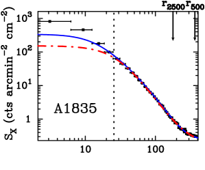
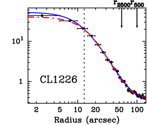
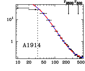
Figure 2: X-ray surface brightness profiles for A1835 (left), CL1226 (middle), and A1914 (right). The vertical dashed line denotes the 100 kpc core cut. In each panel, the blue, solid line is the surface brightness computed using a high-likelihood fit of the N07+SVM profiles (analogous to the SZ models plotted in Fig. 1), while the red, dot-dashed line is that from an isothermal $\beta$-model fit. Both fit lines include the X-ray background that was simultaneously fit with the cluster emission model. The black squares are the annularly-binned X-ray data, where the widths of the bins are denoted by horizonal error bars. The vertical error bars are the 1-$\sigma$ errors on the measurements. Arrows indicate $r_{2500}$ and $r_{500}$ derived from the N07+SVM profiles (see Tables 4 & 5).

The X-ray surface brightness (Eq. 4), ignoring the data within a 100 kpc radius, was modeled separately with both the isothermal $\beta$-model, using the spectroscopically-determined, global $T_{X}$ (measured within $r\in[0.15,1.0]\,r_{500}$), and the SVM, using the temperature derived from the N07 pressure profile fit to the SZ data. Figure 2 shows the maximum-likelihood fits to the surface brightness of each cluster for both the SVM and isothermal $\beta$-model. For plotting purposes, the X-ray data are radially-averaged around the cluster centroid, which is determined in the joint SZ+X-ray analysis by fitting the two-dimensional X-ray imaging data with the spherically-symmetric SVM and isothermal $\beta$-model profiles.

4.3 ICM Profiles

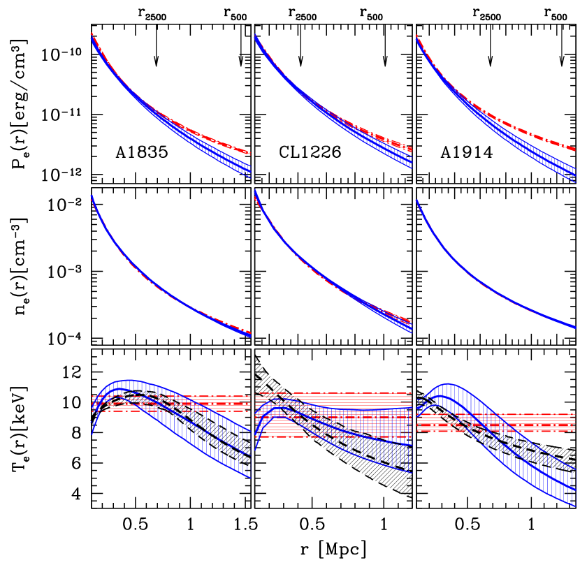
Figure 3: Three-dimensional ICM radial profiles derived from the joint analysis of SZA+Chandra X-ray surface brightness data for A1835, CL1226, and A1914 (from left to right). From top to bottom: the electron pressure $P_{e}(r)$, the electron density $n_{e}(r)$, the derived electron temperature $T_{e}(r)$, profiles as a function of the cluster-centric radius. The lines show the median deprojected quantity derived from data using the N07+SVM (solid lines, vertically-hatched regions) and the isothermal $\beta$-model (dot-dashed lines, horizontally-hatched regions). The derived electron temperature profiles are compared to the spectroscopically-determined radial temperature profiles (black dashed lines, slanted hatching) obtained according to methods presented in M07/M08. The hatched region indicate the 68% confidence on parameters derived from each model. The arrows denote the median values of $r_{2500}$ and $r_{500}$ from the N07+SVM fits.

Figure 3 shows the three-dimensional ICM radial profiles derived from the joint analysis of SZA + Chandra X-ray surface brightness data for A1835, CL1226 and A1914 (from left to right). From top to bottom, we show the electron pressure, the gas density and the derived electron temperature profiles, each as a function of cluster radius. In all panels, we compare the ICM profiles derived from the N07+SVM model to the results of a traditional isothermal $\beta$-model analysis, indicated by solid and dot-dashed lines, respectively. The hatched regions indicate the 68% confidence interval for each derived parameter.

As shown in the top panels of Fig. 3, the pressure profiles derived from the N07 model and the isothermal $\beta$-model show good agreement within $r_{2500}$, but deviate by $\sim$3–5-$\sigma$ in the cluster outskirts. This is a consequence of the fact that clusters exhibit a significant decline in temperature beyond $r_{2500}$, as determined from spectroscopic X-ray observations (see the bottom panel of Fig. 3). The pressure profile derived from the isothermal $\beta$-model analysis is therefore biased systematically high beyond $r_{2500}$. In contrast, the N07 model, which fits the pressure directly, is free to capture the true shape of the pressure profile well beyond the radius at which the assumption of isothermality becomes invalid.

For all three clusters there is little evidence for the second component of the electron density allowed by the SVM; the density is fit equally well by either the SVM or a single-component $\beta$-model, as illustrated by the center row of panels in Fig. 3 (see also Table 2). For all three clusters, the fits of the SVM agree to within 1–2% of the full V06 density profile fits (not shown) outside the core; discrepancies at this level are easily attributed to differences in the fitting of the X-ray background, and to the differences between the APEC and Raymond-Smith emissivity models used respectively in the M07/M08 X-ray analysis and the joint SZ+X-ray analyses.

In the bottom panels, the electron temperature profiles inferred from the N07+SVM profiles are compared to temperature profiles derived from deep spectroscopic Chandra X-ray observations (and XMM-Newton in the case of CL1226; see M07). The comparison shows that the radial electron temperature profiles derived from the N07+SVM profiles are in good agreement with independent X-ray measurements for the relaxed clusters A1835 and CL1226, which exhibit radially decreasing temperature profiles in the cluster outskirts (see also Markevitch et al., 1998; Vikhlinin et al., 2005). The disturbed cluster A1914, however, shows less overall agreement between the derived N07+SVM radial temperature profile and the M08 fit of the V06 temperature profile. Since the N07 pressure profile fit to the SZA observation of A1914 agrees with that derived from M08 within their respective 68% confidence intervals, the temperature discrepancy is likely due to deviations from the spherical symmetry implicitly assumed in this analysis. Additionally, scales greater than about six arcminutes are beyond the radial extents probed by the SZA; it is unsurprising the agreement becomes poorer at radii larger than this.

We note that we fit the SZ data using relativistic corrections to the SZ frequency dependence provided by Itoh et al. (1998). These corrections are appropriate for the thermal SZ effect at the SZA observing frequencies of 30 and 90 GHz. Compared to fits assuming the classical SZ frequency dependence, a pressure profile fit using the relativistic corrections has both a higher normalization and larger upper error bars. This is noticeable when including higher frequency data, where the relativistic correction is larger ($\sim 5\%$ at 90 GHz versus $\sim 3\%$ at 30 GHz for cluster temperatures $\sim$ 8 keV). This increase in the pressure fit is due to the diminished magnitude of the SZ effect when using these corrections (for frequencies below the null in the SZ spectrum, $\lesssim 218$ GHz; see e.g. Itoh et al. (1998)). The pressure profile therefore must adjust to fit the observed SZ flux.

The larger upper error bars on the fit pressure profile arise from a more subtle effect. Since the temperature is derived from the simultaneously fit pressure and density profiles, and the SZ effect diminishes as electrons become more relativistic (i.e. hotter), the upper error bar of the pressure fit must increase to fit the same noise in the observation (compared to the non-relativistic case). The lower error bar is less affected, as lower electron temperatures require smaller relativistic corrections. The resulting asymmetric error bars can be seen in the derived temperature profile of CL1226, which relied on 90 GHz data, in Figure 3.

4.4 Measurements of $Y$, $M_{\mbox{\scriptsize gas}}$, $M_{\mbox{\scriptsize tot}}$, and $f_{\mbox{\scriptsize gas}}$

In Tables 4 and 5, we report global properties of individual clusters derived from the N07+SVM model fits to the SZ+X-ray data. We calculate all quantities at overdensity radii $r_{2500}$ and $r_{500}$, and compare them to results from both the isothermal $\beta$-model analysis of the same data, as well as to the X-ray-only analysis.

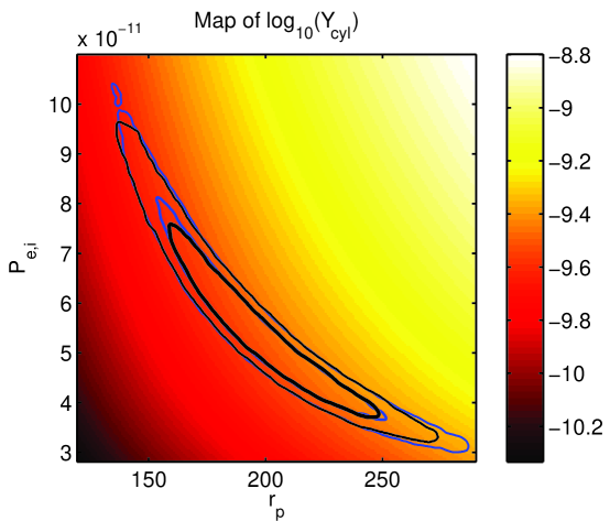
Figure 4: $Y_{\mbox{\scriptsize cyl}}$ computed within 6′ ($\sim 1.4~{}\rm Mpc$, which is $\approx r_{500}$ for this cluster) for fits to SZA observation of A1835. The bold, black contours contain 68% and 95% of the accepted iterations on the jointly-fit Chandra + SZA data, while the thinner, blue contours are those for fits to SZA data alone.

The N07 pressure profile has just two free parameters—$P_{e,i}$ and $r_{p}$—which exhibit a degeneracy. Figure 4 shows this degeneracy in fits of the N07 profile to the SZA observations of A1835. Similar to the $r_{c}-\beta$ degeneracy of the $\beta$-model (see Grego et al., 2001, for example), these two quantities are not individually constrained by our SZ observations, but they are tightly correlated and the preferred region in the $P_{e,i}-r_{p}$ plane encloses approximately constant $Y_{\mbox{\scriptsize cyl}}$. As a result, the 68% confidence region for $Y_{\mbox{\scriptsize cyl}}$ is more tightly constrained than the large variation in $P_{e,i}$ or $r_{p}$ might individually indicate. Figure 4 also shows that the inclusion of X-ray data has only a marginal effect on the value of $Y_{\mbox{\scriptsize cyl}}$ derived from the SZ fit. This is as expected, due to the weak dependence of the X-ray surface brightness on temperature (see § 2.1) and the fact that the N07 profile is not linked to the SVM density profile’s shape. This indicates that X-ray data are not necessary to constrain $Y_{\mbox{\scriptsize cyl}}$, although they do limit the range of accepted radial pressure profiles.

At both $r_{2500}$ and $r_{500}$, the measurements of $Y_{\mbox{\scriptsize cyl}}$ derived from the joint N07+SVM and the X-ray-only analysis are consistent at the 1-$\sigma$ level, for all three clusters. The isothermal $\beta$-model analysis, however, overestimates $Y_{\mbox{\scriptsize cyl}}$ by $\sim$ 20%–40% at $r_{2500}$, and by $\sim$ 30%–115% at $r_{500}$. This is due to the large contribution to $Y_{\mbox{\scriptsize cyl}}$ from the cluster outskirts, at every projected radius, where the $\beta$-model significantly overestimates the pressure.

In contrast to the systematic variations in $Y_{\mbox{\scriptsize cyl}}$, the determinations of $\mbox{$Y_{\mbox{\scriptsize sph}}$}(r_{2500})$ are consistent among the three analyses. At $r_{500}$, however, the median $Y_{\mbox{\scriptsize sph}}$ values from the isothermal $\beta$-model can be as much as $\sim$ 60% higher than either the N07+SVM or M08 results, due to the fact that isothermality is a poor description of the cluster outskirts.

The gas mass estimates computed using either the jointly-fit SVM or the isothermal $\beta$-model agree with the gas masses derived from the Maughan X-ray fits (Tables 4 and 5). This agreement is not surprising, given that the gas mass is determined in all cases from density fits to the X-ray data. It demonstrates, however, that the 100 kpc core makes a negligible contribution to the total gas mass even at $r_{2500}$, and that excluding the core from the joint analysis does not therefore introduce any significant bias in our estimate of $M_{\mbox{\scriptsize gas}}$. Incidentally, it also shows that the additional component allowed by the SVM and the full V06 density models is not indicated in these clusters.

In Tables 4 and 5, we also present estimates of the total masses, computed using each model’s estimate of the overdensity radius ($r_{\Delta}$) for each Monte Carlo realization of the fit parameters. For two of the clusters, we find that the error bars are significantly larger for $M_{\mbox{\scriptsize tot}}$ determined from the N07+SVM fits than for the isothermal $\beta$-model or M08 fits. This is a consequence of the fact that the $\beta$-model analysis, with fewer free parameters and the assumption of isothermality, effectively places stronger but poorly-justified priors on the total mass. We find that the N07+SVM and M08 total mass estimates agree at both $r_{500}$ and $r_{2500}$, leading to good overall agreement between gas fractions computed using the N07+SVM profiles and those from the Maughan X-ray fits.

Since the HSE estimate for $M_{\mbox{\scriptsize tot}}$ is sensitive to the change in slope in the pressure profile ($dP/dr$), $M_{\mbox{\scriptsize tot}}$ is not as well constrained by the N07+SVM profiles as is $Y_{\mbox{\scriptsize cyl}}$, which scales directly with integrated SZ flux, a parameter that is more directly linked to what the SZA observes (see § 4.1). Figure 5 shows a comparison of the N07+SVM estimates for $M_{\mbox{\scriptsize tot}}$ and $Y_{\mbox{\scriptsize cyl}}$, revealing that $Y_{\mbox{\scriptsize cyl}}$ has a more tightly constrained and centrally peaked distribution than $M_{\mbox{\scriptsize tot}}$ does.

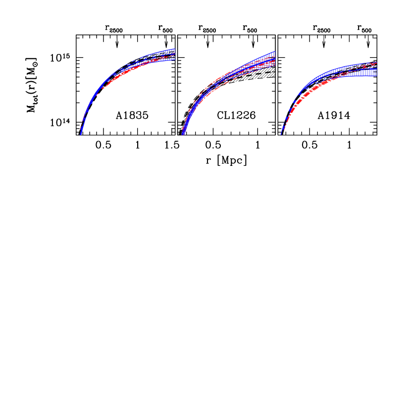
Figure 6: Total mass profiles derived from the joint analysis of SZA+Chandra X-ray surface brightness data for A1835, CL1226, and A1914 (from left to right). The line types are the same as those in Fig. 3.

The isothermal $\beta$-model, on the other hand, is over-constrained such that it cannot agree with the non-isothermal estimates of $M_{\mbox{\scriptsize tot}}$ at both $r_{2500}$ and $r_{500}$, Its estimates of $M_{\mbox{\scriptsize tot}}$ are moreover sensitive to the annulus within which $T_{X}$ is determined (see § 3.3). This trend can be seen in Fig. 6, which shows $M_{\mbox{\scriptsize tot}}$$(r)$ for each cluster.

5 Conclusions

In this work, we demonstrated the application of a new pressure profile, proposed by Nagai et al. (2007), in fitting SZ data taken by the Sunyaev-Zel’dovich Array. By combining the pressure profile constraints from the SZ data with constraints on density from Chandra X-ray imaging, using a simplified form of the density model proposed by Vikhlinin et al. (2006), we were able to determine the properties of three clusters (A1835, A1914, and CL J1226.9+3332) spanning a wide range in redshift and dynamical states.

This technique was compared with two others: a joint analysis of the same SZ + X-ray data relying on the commonly used isothermal $\beta$-model, which assumes the pressure and density profiles have the same form, and an X-ray only analysis that independently models temperature and density using both X-ray imaging and spectroscopic measurements (but excluding SZ data). We find that the global cluster properties at both $r_{2500}$ and $r_{500}$ determined from ICM profiles fit in the joint pressure analysis are in excellent agreement with properties determined in the X-ray analysis. By contrast, the isothermal $\beta$-model tends to overestimate with respect to the other models the gas pressure at $r>r_{2500}$, where isothermality is an increasingly poor assumption. The $\beta$-model thus leads to an overestimate of the cylindrically-integrated Compton $y$-parameter at $r_{500}$. Since the isothermal $\beta$-model does not provide a good description of the ICM profile in the cluster outskirts, we caution against its use in deriving global properties of clusters even at $r\sim r_{500}$, which is a large fraction of the virial radius.

We tested the ability to recover the ICM electron pressure profiles from SZ data by analyzing the SZ data together with the X-ray imaging data alone, ignoring the X-ray spectroscopic information. Assuming the ideal gas law, we derive electron temperature profiles by coupling the pressure fits to the SZ data with the density fits to the X-ray imaging data. We find that these derived temperature profiles show broad agreement with those determined spectroscopically from deep X-ray observations, even for the highest redshift cluster in our sample, at $z=0.89$. This method therefore provides an independent technique for determining the radial electron temperature distribution in high-redshift clusters, for which deep spectroscopic X-ray data may be unavailable and are impractical to obtain.

Table 1: SZA Cluster Observations

Cluster Name	$z$	$D_{A}$	SZA Pointing Center (J2000)		Short Baselines (0.3–1.5 $\rm k\lambda$)		Long Baselines (3.0–7.5 $\rm k\lambda$)		$\rm{\tau_{int,red}}$
		(Gpc)		$\delta$	beam($\arcsec\times\arcsec$)	$\sigma$(mJy)	beam($\arcsec\times\arcsec$)	$\sigma$(mJy)	(hrs)
A1914	0.17	0.60	$14^{h}26^{m}00^{s}\!.8$	$+37^{\circ}49^{\prime}35\arcsec\!.7$	117.5$\times$129.9	0.30	23.5$\times$17.4	0.35	11.5
A1835	0.25	0.81	$14^{h}01^{m}02^{s}\!.0$	$+02^{\circ}52^{\prime}41\arcsec\!.7$	116.6$\times$152.1	0.25	17.5$\times$23.5	0.33	18.6
CL1226 (30-GHz)	0.89	1.60	$12^{h}26^{m}58^{s}\!.0$	$+33^{\circ}32^{\prime}45\arcsec\!.0$	117.4$\times$125.4	0.20	16.0$\times$21.2	0.20	22.0
CL1226 (90-GHz)	”	”	”	”	42.3$\times$39.1	0.42	–	–	29.2

Table 2: Details of X-ray Observations

Cluster Name	ObsID	Joint SZ+X-ray Analysis		Maughan X-ray Analysis
		$\rm{\tau_{int}}$	fitting region	$\rm{\tau_{int}}$	fitting region
		(ks)	″	(ks)	″
A1914	542+3593	26.0	34.4–423.1	23.3	0.0–462.5
A1835	6880	85.7	25.6–344.4	85.7	0.0–519.6
CL1226	3180+5014	64.4	12.9–125.0	50	0.0–125.0
”	0200340101	N/A	N/A	75+68	17.1–115

Table 3: Unresolved Radio Sources in 30-GHz Observations

Cluster Name	Src #	Differential Offset from Pointing Center		Flux at 30.938 GHz
		$\Delta$ R.A. (″)	$\Delta$ Dec. (″)	mJy
A1914	1	-242.1	-235.4	$1.8^{+0.4}_{-0.4}$
A1914	2	-160.5	-108.6	$1.2^{+0.3}_{-0.3}$
A1835	1	0.9	1.5	2.8${}^{+0.3}_{-0.3}$
A1835	2	-22.8	-51.2	1.1${}^{+0.4}_{-0.3}$
A1835	3	-275.1	-178.6	0.8${}^{+0.4}_{-0.4}$
CL1226	1	258.4	-38.9	$3.9^{+0.2}_{-0.2}$

Table 4: $Y_{\rm cyl}$, $Y_{\rm sph}$, $M_{\rm gas}$, $M_{\rm tot}$, and $f_{\rm gas}$ for Each Model Computed Within $r_{2500}$.

Cluster	$\theta_{2500}$	$r_{2500}$	$Y_{\rm cyl}$	$Y_{\rm sph}$	$M_{\rm gas}$	$M_{\rm tot}$	$f_{\rm gas}$
model fit	(″)	(Mpc)	($10^{-5}{\rm Mpc}^{2}$)	($10^{-5}{\rm Mpc}^{2}$)	($10^{13}{\rm M_{\odot}}$)	($10^{14}{\rm M_{\odot}}$)
Abell 1835
N07+SVM	173${}^{+5.8}_{-5.7}$	0.68${}^{+0.02}_{-0.02}$	11.73${}^{+1.36}_{-1.27}$	8.25${}^{+0.81}_{-0.78}$	5.74${}^{+0.26}_{-0.25}$	5.64${}^{+0.58}_{-0.54}$	0.102${}^{+0.006}_{-0.005}$
Maughan (this work)	169${}^{+5.5}_{-8.0}$	0.66${}^{+0.02}_{-0.03}$	11.58${}^{+0.61}_{-0.67}$	7.88${}^{+0.49}_{-0.72}$	5.77${}^{+0.25}_{-0.35}$	5.30${}^{+0.53}_{-0.72}$	0.109${}^{+0.009}_{-0.006}$
isothermal $\beta$-model	159${}^{+3.0}_{-2.9}$	0.62${}^{+0.01}_{-0.01}$	13.85${}^{+0.72}_{-0.67}$	7.94${}^{+0.43}_{-0.40}$	4.96${}^{+0.13}_{-0.12}$	4.38${}^{+0.25}_{-0.24}$	0.113${}^{+0.004}_{-0.004}$
CL J1226+3332.9
N07+SVM	52.8${}^{+1.8}_{-1.9}$	0.41${}^{+0.01}_{-0.01}$	5.49${}^{+0.53}_{-0.50}$	3.56${}^{+0.36}_{-0.36}$	2.91${}^{+0.14}_{-0.14}$	2.67${}^{+0.29}_{-0.27}$	0.109${}^{+0.007}_{-0.007}$
Maughan et al. (2007)	57.3${}^{+1.6}_{-1.5}$	0.45${}^{+0.01}_{-0.01}$	7.57${}^{+0.33}_{-0.34}$	5.04${}^{+0.31}_{-0.28}$	3.25${}^{+0.14}_{-0.13}$	3.41${}^{+0.30}_{-0.26}$	0.095${}^{+0.004}_{-0.004}$
isothermal $\beta$-model	54.2${}^{+5.1}_{-4.3}$	0.42${}^{+0.04}_{-0.03}$	6.76${}^{+0.91}_{-0.73}$	3.92${}^{+0.60}_{-0.48}$	2.93${}^{+0.40}_{-0.33}$	2.89${}^{+0.90}_{-0.63}$	0.101${}^{+0.014}_{-0.014}$
Abell 1914
N07+SVM	228${}^{+12.9}_{-11.7}$	0.67${}^{+0.04}_{-0.03}$	8.43${}^{+1.55}_{-1.24}$	6.29${}^{+1.03}_{-0.82}$	4.71${}^{+0.34}_{-0.30}$	4.97${}^{+0.89}_{-0.72}$	0.095${}^{+0.009}_{-0.009}$
Maughan et al. (2008)	218${}^{+7.1~{}}_{-5.7~{}}$	0.63${}^{+0.02}_{-0.02}$	7.87${}^{+0.56}_{-0.55}$	5.69${}^{+0.37}_{-0.38}$	4.64${}^{+0.17}_{-0.16}$	4.31${}^{+0.43}_{-0.33}$	0.107${}^{+0.005}_{-0.006}$
isothermal $\beta$-model	204${}^{+5.7~{}}_{-5.1~{}}$	0.59${}^{+0.02}_{-0.01}$	11.28${}^{+0.59}_{-0.56}$	6.24${}^{+0.34}_{-0.32}$	4.04${}^{+0.15}_{-0.14}$	3.52${}^{+0.30}_{-0.26}$	0.115${}^{+0.005}_{-0.005}$

Table 5: $Y_{\rm cyl}$, $Y_{\rm sph}$, $M_{\rm gas}$, $M_{\rm tot}$, and $f_{\rm gas}$ for Each Model Computed Within $r_{500}$.

Cluster	$\theta_{500}$	$r_{500}$	$Y_{\rm cyl}$	$Y_{\rm sph}$	$M_{\rm gas}$	$M_{\rm tot}$	$f_{\rm gas}$
model fit	(″)	(Mpc)	($10^{-5}{\rm Mpc}^{2}$)	($10^{-5}{\rm Mpc}^{2}$)	($10^{13}{\rm M_{\odot}}$)	($10^{14}{\rm M_{\odot}}$)
Abell 1835
N07+SVM	369${}^{+28}_{-27}$	1.44${}^{+0.11}_{-0.10}$	20.79${}^{+3.79}_{-3.34}$	17.55${}^{+3.00}_{-2.70}$	13.67${}^{+1.03}_{-1.01}$	11.00${}^{+2.68}_{-2.22}$	0.124${}^{+0.020}_{-0.017}$
Maughan (this work)	363${}^{+17}_{-12}$	1.42${}^{+0.07}_{-0.05}$	21.37${}^{+2.45}_{-1.58}$	17.41${}^{+1.61}_{-0.99}$	13.94${}^{+0.64}_{-0.52}$	10.68${}^{+1.54}_{-1.01}$	0.133${}^{+0.009}_{-0.012}$
isothermal $\beta$-model	361${}^{+7~{}}_{-6~{}}$	1.41${}^{+0.03}_{-0.03}$	34.53${}^{+1.78}_{-1.68}$	21.29${}^{+1.09}_{-1.02}$	13.29${}^{+0.27}_{-0.27}$	10.30${}^{+0.58}_{-0.54}$	0.129${}^{+0.005}_{-0.005}$
CL J1226+3332.9
N07+SVM	127${}^{+13}_{-10}$	0.98${}^{+0.10}_{-0.07}$	11.9${}^{+2.0}_{-1.6}$	9.71${}^{+1.58}_{-1.29}$	8.50${}^{+0.68}_{-0.60}$	7.37${}^{+2.50}_{-1.57}$	0.115${}^{+0.022}_{-0.023}$
Maughan et al. (2007)	115${}^{+3~{}}_{-3~{}}$	0.89${}^{+0.02}_{-0.02}$	13.9${}^{+1.3}_{-1.1}$	10.59${}^{+0.69}_{-0.68}$	8.30${}^{+0.32}_{-0.36}$	5.49${}^{+0.46}_{-0.47}$	0.151${}^{+0.008}_{-0.008}$
isothermal $\beta$-model	126${}^{+11}_{-9}$	0.98${}^{+0.09}_{-0.07}$	16.8${}^{+1.9}_{-1.6}$	10.97${}^{+1.30}_{-1.06}$	8.21${}^{+0.77}_{-0.65}$	7.30${}^{+2.10}_{-1.51}$	0.113${}^{+0.018}_{-0.018}$
Abell 1914
N07+SVM	430${}^{+38}_{-33}$	1.25${}^{+0.11}_{-0.10}$	12.90${}^{+2.97}_{-2.31}$	11.05${}^{+2.44}_{-1.91}$	10.26${}^{+0.94}_{-0.85}$	6.62${}^{+1.90}_{-1.42}$	0.155${}^{+0.026}_{-0.023}$
Maughan et al. (2008)	448${}^{+24}_{-21}$	1.29${}^{+0.07}_{-0.06}$	13.47${}^{+1.68}_{-1.77}$	10.78${}^{+1.03}_{-1.09}$	10.24${}^{+0.45}_{-0.57}$	7.49${}^{+1.29}_{-1.00}$	0.138${}^{+0.015}_{-0.018}$
isothermal $\beta$-model	461${}^{+13}_{-11}$	1.34${}^{+0.04}_{-0.03}$	29.08${}^{+1.52}_{-1.44}$	17.07${}^{+0.87}_{-0.84}$	11.05${}^{+0.36}_{-0.33}$	8.14${}^{+0.69}_{-0.59}$	0.136${}^{+0.007}_{-0.007}$

Figure 5: 1-D histograms of $M_{\mbox{\scriptsize tot}}$ (cyan/light gray region with dashed outline) and $Y_{\mbox{\scriptsize cyl}}$ (vertically-hatched region with solid outline), normalized by their respective median values, derived from the joint fits of the N07+SVM profiles to A1835. Both $M_{\mbox{\scriptsize tot}}$ and $Y_{\mbox{\scriptsize cyl}}$ are computed within a fixed radius of $\theta=6\arcmin$. The derived $Y_{\mbox{\scriptsize cyl}}$, which scales directly with integrated SZ flux, has a more tightly constrained and centrally peaked distribution than that of $M_{\mbox{\scriptsize tot}}$, as $M_{\mbox{\scriptsize tot}}$ is sensitive to the change in slope in the pressure profile ($dP/dr$).

References

- Allen et al. (2007) Allen, S. W., Rapetti, D. A., Schmidt, R. W., Ebeling, H., Morris, G., & Fabian, A. C. 2007, ArXiv e-prints, 706
- Anders & Grevesse (1989) Anders, E. & Grevesse, N. 1989, Geochim. Cosmochim. Acta, 53, 197
- Atrio-Barandela et al. (2008) Atrio-Barandela, F., Kashlinsky, A., Kocevski, D., & Ebeling, H. 2008, ApJ, 675, L57
- Bonamente et al. (2008) Bonamente, M., Joy, M., LaRoque, S. J., Carlstrom, J. E., Nagai, D., & Marrone, D. P. 2008, ApJ, 675, 106
- Bonamente et al. (2004) Bonamente, M., Joy, M. K., Carlstrom, J. E., Reese, E. D., & LaRoque, S. J. 2004, ApJ, 614, 56
- Bonamente et al. (2006) Bonamente, M., Joy, M. K., LaRoque, S. J., Carlstrom, J. E., Reese, E. D., & Dawson, K. S. 2006, ApJ, 647, 25
- Carlstrom et al. (2002) Carlstrom, J. E., Holder, G. P., & Reese, E. D. 2002, ARA&A, 40, 643
- Cavaliere & Fusco-Femiano (1976) Cavaliere, A. & Fusco-Femiano, R. 1976, A&A, 49, 137
- Cavaliere & Fusco-Femiano (1978) —. 1978, A&A, 70, 677
- Condon et al. (1998) Condon, J. J., Cotton, W. D., Greisen, E. W., Yin, Q. F., Perley, R. A., Taylor, G. B., & Broderick, J. J. 1998, AJ, 115, 1693
- da Silva et al. (2004) da Silva, A. C., Kay, S. T., Liddle, A. R., & Thomas, P. A. 2004, MNRAS, 348, 1401
- Dobbs et al. (2006) Dobbs, M., Halverson, N. W., Ade, P. A. R., Basu, K., Beelen, A., Bertoldi, F., Cohalan, C., Cho, H. M., Güsten, R., Holzapfel, W. L., Kermish, Z., Kneissl, R., Kovács, A., Kreysa, E., Lanting, T. M., Lee, A. T., Lueker, M., Mehl, J., Menten, K. M., Muders, D., Nord, M., Plagge, T., Richards, P. L., Schilke, P., Schwan, D., Spieler, H., Weiss, A., & White, M. 2006, New Astronomy Review, 50, 960
- Ebeling et al. (2001) Ebeling, H., Edge, A. C., & Henry, J. P. 2001, ApJ, 553, 668
- Frenk et al. (1999) Frenk, C. S., White, S. D. M., Bode, P., Bond, J. R., Bryan, G. L., Cen, R., Couchman, H. M. P., Evrard, A. E., Gnedin, N., Jenkins, A., Khokhlov, A. M., Klypin, A., Navarro, J. F., Norman, M. L., Ostriker, J. P., Owen, J. M., Pearce, F. R., Pen, U.-L., Steinmetz, M., Thomas, P. A., Villumsen, J. V., Wadsley, J. W., Warren, M. S., Xu, G., & Yepes, G. 1999, ApJ, 525, 554
- Gilks et al. (1996) Gilks, W. R., Richardson, S., & Spiegelhalter, D. J. 1996, Markov Chain Monte Carlo in Practice (Chapman and Hall)
- Grego et al. (2000) Grego, L., Carlstrom, J. E., Joy, M. K., Reese, E. D., Holder, G. P., Patel, S., Cooray, A. R., & Holzapfel, W. L. 2000, ApJ, 539, 39
- Grego et al. (2001) Grego, L., Carlstrom, J. E., Reese, E. D., Holder, G. P., Holzapfel, W. L., Joy, M. K., Mohr, J. J., & Patel, S. 2001, ApJ, 552, 2
- Haiman et al. (2001) Haiman, Z., Mohr, J. J., & Holder, G. P. 2001, ApJ, 553, 545
- Itoh et al. (1998) Itoh, N., Kohyama, Y., & Nozawa, S. 1998, ApJ, 502, 7
- Kosowsky (2003) Kosowsky, A. 2003, New Astronomy Review, 47, 939
- LaRoque et al. (2006) LaRoque, S. J., Bonamente, M., Carlstrom, J. E., Joy, M. K., Nagai, D., Reese, E. D., & Dawson, K. S. 2006, ApJ, 652, 917
- Markevitch et al. (1998) Markevitch, M., Forman, W. R., Sarazin, C. L., & Vikhlinin, A. 1998, ApJ, 503, 77
- Maughan et al. (2008) Maughan, B. J., Jones, C., Forman, W., & Van Speybroeck, L. 2008, ApJS, 174, 117
- Maughan et al. (2007) Maughan, B. J., Jones, C., Jones, L. R., & Van Speybroeck, L. 2007, ApJ, 659, 1125
- Maughan et al. (2004) Maughan, B. J., Jones, L. R., Ebeling, H., & Scharf, C. 2004, MNRAS, 351, 1193
- Motl et al. (2005) Motl, P. M., Hallman, E. J., Burns, J. O., & Norman, M. L. 2005, ApJ, 623, L63
- Muchovej et al. (2007) Muchovej, S., Mroczkowski, T., Carlstrom, J. E., Cartwright, J., Greer, C., Hennessy, R., Loh, M., Pryke, C., Reddall, B., Runyan, M., Sharp, M., Hawkins, D., Lamb, J. W., Woody, D., Joy, M., Leitch, E. M., & Miller, A. D. 2007, ApJ, 663, 708
- Nagai (2006) Nagai, D. 2006, ApJ, 650, 538
- Nagai et al. (2007) Nagai, D., Kravtsov, A. V., & Vikhlinin, A. 2007, ApJ, 668, 1
- Navarro et al. (1997) Navarro, J. F., Frenk, C. S., & White, S. D. M. 1997, ApJ, 490, 493
- Peterson et al. (2001) Peterson, J. R., Paerels, F. B. S., Kaastra, J. S., Arnaud, M., Reiprich, T. H., Fabian, A. C., Mushotzky, R. F., Jernigan, J. G., & Sakelliou, I. 2001, A&A, 365, L104
- Piffaretti et al. (2005) Piffaretti, R., Jetzer, P., Kaastra, J. S., & Tamura, T. 2005, A&A, 433, 101
- Pratt & Arnaud (2002) Pratt, G. W. & Arnaud, M. 2002, A&A, 394, 375
- Pratt et al. (2007) Pratt, G. W., Böhringer, H., Croston, J. H., Arnaud, M., Borgani, S., Finoguenov, A., & Temple, R. F. 2007, A&A, 461, 71
- Raftery & Lewis (1992) Raftery, A. L. & Lewis, S. 1992, in Bayesian Statistics IV, ed. J. M. Bernardo & M. H. DeGroot (Oxford University Press), 763
- Raymond & Smith (1977) Raymond, J. C. & Smith, B. W. 1977, ApJS, 35, 419
- Reese et al. (2002) Reese, E. D., Carlstrom, J. E., Joy, M., Mohr, J. J., Grego, L., & Holzapfel, W. L. 2002, ApJ, 581, 53
- Reid & Spergel (2006) Reid, B. A. & Spergel, D. N. 2006, ApJ, 651, 643
- Rudy (1987) Rudy, D. J. 1987, PhD thesis, California Institute of Technology
- Ruhl et al. (2004) Ruhl, J. E., Ade, P. A. R., Carlstrom, J. E., Cho, H. M., Crawford, T., Dobbs, M., Greer, C. H., Halverson, N. W., Holzapfel, W. L., Lantin, T. M., Lee, A. T., Leong, J., Leitch, E. M., Lu, W., Lueker, M., Mehl, J., Meyer, S. S., Mohr, J. J., Padin, S., Plagge, T., Pryke, C., Schwan, D., Sharp, M. K., Runyan, M. C., Spieler, H., Staniszewski, Z., & Stark, A. A. 2004, astro-ph/0411122
- Sarazin (1988) Sarazin, C. L. 1988, X-ray Emission From Clusters of Galaxies (Cambridge University Press)
- Shepherd (1997) Shepherd, M. C. 1997, in Astronomical Society of the Pacific Conference Series, Vol. 125, Astronomical Data Analysis Software and Systems VI, ed. G. Hunt & H. Payne, 77
- Smith et al. (2001) Smith, R. K., Brickhouse, N. S., Liedahl, D. A., & Raymond, J. C. 2001, ApJ, 556, L91
- Struble & Rood (1999) Struble, M. F. & Rood, H. J. 1999, ApJS, 125, 35
- Sunyaev & Zel’dovich (1970) Sunyaev, R. A. & Zel’dovich, Y. B. 1970, Comments Astrophys. Space Phys., 2, 66
- Sunyaev & Zel’dovich (1972) —. 1972, Comments Astrophys. Space Phys., 4, 173
- Thompson et al. (2001) Thompson, A. R., Moran, J. M., & Swenson, G. W. 2001, Interferometry and Synthesis in Radio Astronomy (Wiley-Interscience, 2nd ed.)
- Vikhlinin et al. (2006) Vikhlinin, A., Kravtsov, A., Forman, W., Jones, C., Markevitch, M., Murray, S. S., & Van Speybroeck, L. 2006, ApJ, 640, 691
- Vikhlinin et al. (2005) Vikhlinin, A., Markevitch, M., Murray, S. S., Jones, C., Forman, W., & Van Speybroeck, L. 2005, ApJ, 628, 655
- Weller et al. (2002) Weller, J., Battye, R. A., & Kneissl, R. 2002, Physical Review Letters, 88, 231301
- White et al. (1997) White, R. L., Becker, R. H., Helfand, D. J., & Gregg, M. D. 1997, ApJ, 475, 479
- White et al. (1993) White, S. D. M., Efstathiou, G., & Frenk, C. S. 1993, MNRAS, 262, 1023