The Passage of Ultrarelativistic Neutralinos through the Matter of the Moon

Abstract

I consider the prospect to use the outer layer of the Moon as a detector volume for ultra–high energy (UHE) neutrino fluxes and the flux of the lightest neutralino which I assume is the lightest supersymmetric particle (LSP). For this purpose, I calculate the event rates of these fluxes for top–down scenarios. I show that a suitable experiment for the detection of radio waves might be able to detect sufficient event rates after a measurement period of one year.

1 Introduction

A promising idea, which was first suggested by Dagkesamanskii and Zheleznyk Dagkesamanskii , for the detection of UHE particle fluxes like ultrarelativistic neutralinos or neutrinos is the measurement of radio waves when these particles hit the Moon gorhamandcoexp . These radio waves are produced due to the Askaryan effect askara and the emission of Cerenkov radiation, respectively. UHE particles cause a cascade of secondary particles when they are interacting in the Moon’s matter. This cascade develops a cloud of negative charge in a dense dielectric medium because electrons are entrained from the surrounding matter. As a result, Cerenkov light is produced since these electrons are moving with a velocity which is faster than the velocity of light in the medium. Coherence builds up for the range of wavelengths which is about the dimension of the cloud; the wavelengths of radio frequencies are just comparable to the dimension of the electron shower James:2008ff . Therefore we can use a part of the outer layer of the Moon as an effective detector volume.

2 Equations for the Event Rates

This section outlines the derivation of the event rates ${\cal N}$ using the Moon as a detector; I refer to Bornhauser:2006ve ; Bornhauser:2007sw ; dissertation for a detailed derivation. The event rates for UHE higgsino–like LSPs where the cross section $\sigma_{t}$ is dominated by the t–channel contributions Bornhauser:2006ve is given by:

$${\cal N}_{t} = \int_{E_{\rm min}}^{E_{\rm max}}dE_{\rm vis}\int_{{\bf X}_{\rm min}}^{{\bf X}_{\rm max}}d{\bf X}\int_{0}^{1}dy\frac{1}{y}F_{\tilde{\chi}_{1}^{0}}(\frac{E_{\rm vis}}{y},{\bf X})\cdot$$ (1)

$$\left(G_{\tilde{\chi}_{1}^{0}}^{\rm NC}(E_{\rm vis},y)+G_{\tilde{\chi}_{1}^{0}}^{\rm CC}(E_{\rm vis},y)\right){\mathcal{V}}\,,$$

where the constant factor ${\mathcal{V}}$ is given by

$${\mathcal{V}}\equiv 2\pi V_{\rm eff}\epsilon_{\rm DC}tN_{A}\rho_{w}J_{D}\,$$ (2)

and the convolutions of Eq. (1) are given by

$$G_{\tilde{\chi}_{1}^{0}}^{NC,CC}(E_{\rm vis},y) = \int_{z}^{z_{1,{\rm max}}}\frac{d\!z_{1}}{z_{1}}\frac{d\sigma^{NC,CC}_{t_{\tilde{\chi}}}(\frac{E_{\rm vis}}{y},z_{1})}{dz_{1}}\cdot$$ (3)

$$\frac{1}{\Gamma}\left.\frac{d\Gamma_{\tilde{\chi}_{\rm out}}(z_{1}\frac{E_{\rm vis}}{y},z_{2}=\frac{z}{z_{1}})}{dz_{2}}\right|_{z=1-y}\,.$$

Here, $E_{\rm vis}=E_{\tilde{\chi}^{0}_{1,{\rm in}}}-E_{\tilde{\chi}^{0}_{1,{\rm out}}}=yE_{\tilde{\chi}^{0}_{1,\rm in}}$ denotes the visible Energy, where $E_{\tilde{\chi}^{0}_{1,{\rm in}}}$ ($E_{\tilde{\chi}^{0}_{1,{\rm out}}}$) is the energy of the LSP before (after) the scattering ($\tilde{\chi}_{1}^{0}$–nucleon scattering always produces another $\tilde{\chi}_{1}^{0}$ in the final state Bornhauser:2006ve ). X denotes the column depth, measured in g/cm² and $F_{\tilde{\chi}_{1}^{0}}$ the differential neutralino LSP flux. The $\tilde{\chi}_{1}^{0}$ flux with matter leads to fluxes of $\tilde{\chi}_{1}^{\pm}$ (charged current (CC) scattering) and $\tilde{\chi}_{2}^{0}$ (neutral current (NC) scattering) Bornhauser:2006ve , collectively denoted by $\tilde{\chi}_{\rm out}$; $z_{1}=E_{\tilde{\chi}_{\rm out}}/E_{\tilde{\chi}^{0}_{1,{\rm in}}}$ describes the energy transfer from the incoming lightest neutralino to the heavier neutralino or chargino, and $z_{2}=E_{\tilde{\chi}^{0}_{1,{\rm out}}}/E_{\tilde{\chi}_{\rm out}}$ describes the energy transfer from this heavier neutralino or chargino to the lightest neutralino produced in its decay. $z_{2}$ is chosen such that $z\equiv z_{1}z_{2}=1-y$; the missing pieces in Eq.(3) are the total and differential decay spectrum of the produced $\tilde{\chi}_{\rm out}$, see Bornhauser:2006ve . Finally, the constant factor ${\mathcal{V}}$ is given by

$${\mathcal{V}}\equiv 2\pi V_{\rm eff}\epsilon_{\rm DC}tN_{A}\rho_{w}J_{D}\,.$$ (4)

Here, $V_{\rm eff}$ is the water equivalent effective volume, $\epsilon_{DC}$ is the duty cycle (the fraction of time where the experiment can observe events), $t$ is the observation time, $N_{A}=6.022\times 10^{23}\mbox{~{}g}^{-1}$ is Avogadro’s number, $\rho_{w}=10^{6}\mbox{~{}g}\mbox{m}^{-3}$ is the density of water, and $J_{D}=\mid\!d\cos\theta_{E}/d{\bf X}\!\mid$ is the Jacobian for the transformation $\cos\theta_{E}\rightarrow{\bf X}(\cos\theta_{E})$, where $\theta_{E}$ is the Earth–zenith angle.

The event rates for the three species of neutrinos are given by:

$${\cal N_{\nu_{\mu,\tau}}} = \int d{\mathcal{M}}\frac{1}{y}F_{\nu_{\mu,\tau}}(\frac{E_{\rm vis}}{y},{\bf X}(\theta^{\prime},\phi^{\prime},r^{\prime},\phi))\cdot$$ (5)

$$\left(\frac{d\sigma_{t_{\nu}}^{\rm NC}(\frac{E_{\rm vis}}{y},y)}{dy}+\frac{d\sigma_{t_{\nu}}^{\rm CC}(\frac{E_{\rm vis}}{y},y)}{dy}\right){\mathcal{V}}^{\prime}\,,$$

$${\cal N}_{\nu_{e}} = \int d{\mathcal{M}}\frac{1}{y}F_{\nu_{e}}(\frac{E_{\rm vis}}{y},{\bf X}(\theta^{\prime},\phi^{\prime},r^{\prime},\phi))\cdot$$ (6)

$$\left(\frac{d\sigma_{t_{\nu}}^{\rm NC}(\frac{E_{\rm vis}}{y},y)}{dy}+N_{\nu_{e}}^{\rm CC}(E_{\rm vis},y)\right){\mathcal{V}}^{\prime}\,,$$

where

$${\cal N}_{\nu_{e}}^{\rm CC}(E_{\rm vis},y)=\delta\!(y-1)\sigma_{t_{\nu}}^{\rm CC}(E_{\rm vis})\,,$$ (7)

where ${\mathcal{V}}$ is now replaced by

$${\mathcal{V}}^{\prime}\equiv\epsilon_{\rm DC_{M}}tN_{A}\rho_{M}\,.$$ (8)

and $\int d{\mathcal{M}}$ is a placeholder for the six integrations:

$$\int d{\mathcal{M}} = \int_{E_{\rm min}}^{E_{\rm max}}dE_{\rm vis}\int_{0}^{1}dy\int_{0}^{\pi/2}d\theta^{\prime}\underbrace{\int_{0}^{2\pi}d{\phi}^{\prime}}_{=2\pi}\cdot$$

$$\int_{r_{M-10m}}^{r_{M}}d{r^{\prime}}{r^{\prime}}^{2}\sin{\theta}^{\prime}\int_{0}^{2\pi}d\phi\int_{53.5^{\circ}}^{56.5^{\circ}}d\theta\sin\theta\,.$$

The primed variables $\theta^{\prime},\phi^{\prime},r^{\prime}$ denote the spherical coordinates for the integration over the allowed volume of the Moon, c. f.  dissertation ; the unprimed variables $\phi,\theta$ are used for the parametrization of the cone of all particle trajectories which can be detected at Earth dissertation . $\theta$ denotes the angle of incidence (roughly the Cerenkov light angle $\theta_{C}$) of the UHE particles with respect to the $z-$axis of the spherical coordinates, which is orientated in direction to the Earth; $\phi$ determines the exact position of a trajectory on the circle around the $z-$axis of the cone for a fixed value of $\theta$. The density of the surface layer of the Moon (regolith) is given by $\rho_{M}=1.7\cdot 10^{6}\mbox{~{}g}\mbox{m}^{-3}$ Stal:2006te ; James:2008ff .

3 Numerical Results

I assume that an experiment for the detection of radio waves produced by Cerenkov radiation can cover one half of the Moon’s surface. From this I deduce that one has an effective detector volume of about $320$ teratons, if the Cerenkov light can leave the regolith up to depth of roughly $10$ m Stal:2006te ; James:2008ff . Furthermore, I expect that the Moon appears 40% of the time above the radio telescope and I assume a lower bound for the visible energy of $10^{10}$ GeV.

I study top-down scenarios with $X$–particle masses of $M_{X}=10^{12}$ and $M_{X}=10^{16}$ GeV for four different primary decay modes, where the corresponding fluxes at source were generated with SHdecay cyrille . The event rates are calculated for all three neutrino flavors and higgsino–like neutralino LSPs. The results are given in Tab. 1.

Mode	$N_{\mu,\tau}^{\nu}$	$N_{e}^{\nu}$	$N_{\rm total}^{\nu}$	$N_{\tilde{\chi}_{1}^{0}}$
$E_{\rm vis}\geq 10^{10}$ GeV, $M_{X}=10^{12}$ GeV
$q\bar{q}$	$0.38$	$1.70$	$2.46$	$0.10$
$q\tilde{q}$	$0.72$	$2.81$	$4.25$	$1.10$
$l\tilde{l}$	$14.76$	$35.52$	$65.04$	$60.10$
$5\times q\tilde{q}$	$1.66$	$7.97$	$11.29$	$1.22$
$E_{\rm vis}\geq 10^{10}$ GeV, $M_{X}=10^{16}$ GeV
$q\bar{q}$	$1.97$	$4.44$	$8.38$	$0.04$
$q\tilde{q}$	$1.27$	$2.98$	$5.52$	$0.05$
$l\tilde{l}$	$1.46$	$3.17$	$6.09$	$0.19$
$5\times q\tilde{q}$	$1.13$	$2.71$	$4.97$	$0.07$

Table 1: Event rates for the scenario H2 of Bornhauser:2006ve ; third column shows the sum of the three neutrino fluxes. I show results for $X$–particle decays into a quark antiquark pair (“$q\bar{q}$”), into a quark squark pair (“$q\tilde{q}$”), into a lepton slepton pair (“$l\tilde{l}$”), and into five quarks and five squarks (“$5\times q\tilde{q}$”).

The tau and muon neutrino fluxes have the same equations for the event rates $N_{\mu,\tau}^{\nu}$ due to their equal behaviour regarding the energy loss of their corresponding leptons produced by CC interactions dissertation . Similarly, the different properties of electrons with respect to their energy loss in matter give rise to electron neutrino event rates $N_{e}^{\nu}$ being always higher than $N_{\mu}^{\nu}$. It is assumed for Eq. (6) that electron neutrinos give $100\%$ of their energy to the visible energy when they undergo a CC interaction. I take the same initial spectrum for all three flavors of neutrinos since the total neutrino flux impinging on the Earth roughly split up to one third per each flavor due to near–maximal neutrino flavor mixing. In addition, the change of the initial spectra by reason of their interaction with Moon’s matter is equal for all three neutrino fluxes, c. f. dissertation .

As shown in bdhh2 , the expected neutralino LSP flux depends quite strongly on $M_{X}$ as well as on the dominant $X$–particle decay mode. Top–down models predict rather hard spectra, i.e. $E^{3}$ times the flux increases with energy. Our fixing of the normalization of the fluxes through the (proton) flux at $E=10^{20}$ eV leads to smaller fluxes at $E<10^{20}$ eV as $M_{X}$ is increased. Moreover, if $M_{X}$ is not far from its lower bound of $\sim 10^{12}$ GeV, much of the relevant neutralino flux is produced early in the parton cascade triggered by $X$ decay, which is quite sensitive to the primary $X$ decay mode. In contrast, if $M_{X}\gg 10^{12}$ GeV, in the relevant energy range most LSPs originate quite late in the cascade; in that case the LSP spectrum is largely determined by the dynamics of the cascade itself, which only depends on Standard Model interactions, and is not very sensitive to the primary $X$ decay mode(s). We also see in Tab. 1 that in case of the neutrino fluxes all four decay modes, independent of the $X$–particle mass, might lead to an observable signal. The neutralino LSP fluxes yield only detectable signals for $M_{X}=10^{12}$ GeV and the last three decay modes, where the decay into a lepton plus a slepton is the most favorable one. The reason is that this decay mode leads to a rather small number of protons produced per $X$ decay, or, put differently, to a large ratio of the LSP and proton fluxes cyrille . Since I normalize to the proton flux, this then leads to a rather large LSP flux. As explained above the event rates for the higher $X$–particle mass are quite independent from the primary decay mode, whereas this correlation is still given for the results of the lower $X$–particle mass.

For $M_{X}=10^{12}$ GeV and both the second and third decay mode the total event rates might have the same order of magnitude with respect to the neutralino LSP and neutrino fluxes. This gives rise to the question how we can disentangle both signals; this question is important for the discrimination between bottom–up and top–down models. For this purpose, I consider the angular dependence of the signals, which is displayed in Fig. 1.

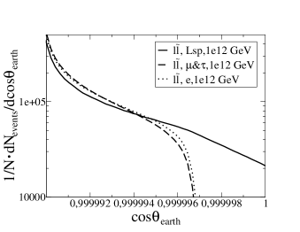
Figure 1: Angular dependence of the signals of neutrinos and higgsino–like neutralino LSPs from primary $X\rightarrow l\tilde{l}$ decays. The solid curve shows the differential event rate for the neutralino flux and the dotted and dashed curves show the differential event rate for the electron and tau/muon neutrino flux, respectively.

Here, the normalized differential event rate is plotted against the angle $\theta_{earth}$ given by the angle relative to the center of the Moon at Earth which describes the deviation from the connecting line between the Earth’s and Moon’s center, see dissertation ; the smaller this angle the smaller is the distance from the connecting line of Earth–Moon. That means larger averaged travel distances for the UHE particles in the Moon’s matter. Therefore, the attenuation of the neutrino fluxes is higher compared to the neutralino LSP fluxes for such angles. The former fluxes are negligible for $\theta_{earth}\geq 0.999997$ as shown by Fig. 1, what give rise to the requirement of an angle resolution of at least $0.14^{\circ}$ for a radio wave antenna experiment if we want to discriminate between signals caused by neutralino LSPs and neutrinos.

4 Conclusion

I have shown that a measurement period of one year already might lead to detectable event rates of UHE neutrinos for both $X$–particle masses, $10^{12}$ and $10^{16}$ GeV, and all four primary decay modes. The above measurement period might lead in the case of UHE neutralino LSPs to a measurable signal if the $X$–particles have masses close to their lower bound of $\sim 10^{12}$ GeV and decay mainly via the last three primary decay modes and modes with a large ratio of neutralino LSP and proton fluxes, respectively. In case of $X$–particles with mass $10^{16}$ GeV one would need at least ten years of detection, even for the most favorable scenario, to collect a observable event rate. The event rates for UHE neutralino LSPs and neutrinos have the same order of magnitude for two of the considered primary decay modes for $X$–particles masses of $10^{12}$ GeV; the disentanglement between the neutralino LSP and neutrino signal is only possible for a radio wave antenna experiment having a angle resolution of at least $0.14^{\circ}$.

References

- (1) R. D. Dagkesamanskii and I. M. Zheleznyk, Sov. Phys. JETP 50, 233 (1989).
- (2) P. W. Gorham et al., PRL 93 (2004) 041101; T. H. Hankins, R. D. Ekers, J. D. O’Sullivan, MNRAS 283 (1996) 1027; A. R. Beresnyak, R. D. Dagkesamanskii, I. M. Zheleznykh, A. V. Kovalenko, V. V. Oreshko, Astronomy Reports 49 (2005) 127; E. Zas, F. Halzen and T. Stanev, Phys. Rev. D 45, 362 (1992); J. Alvarez-Muniz and E. Zas, AIP Conf. Proc. 579, 128 (2001) [arXiv:astro-ph/0102173]; P. W. Gorham, K. M. Liewer, C. J. Naudet, D. P. Saltzberg and D. R. Williams, arXiv:astro-ph/0102435; A. R. Beresnyak, arXiv:astro-ph/0310295; C. W. James, R. M. Crocker, R. D. Ekers, T. H. Hankins, J. D. O’Sullivan, R. J. Protheroe, MNRAS 379 (2007) 3.
- (3) G. A. Askaryan, Sov. Phys. JETP 14,441 (1962); 21, 658 (1965)
- (4) C. W. James and R. J. Protheroe, arXiv:0802.3562 [astro-ph].
- (5) S. Bornhauser and M. Drees, Astropart. Phys. 27 (2007) 30 [arXiv:hep-ph/0603162].
- (6) S. Bornhauser and M. Drees, Phys. Lett. B 650 (2007) 407 [arXiv:0704.3934 [hep-ph]].
- (7) PhD Thesis; Link: “http://hss.ulb.uni-bonn.de/diss_online/ math_nat_fak/2008/bornhauser_sascha/index.htm”
- (8) O. Stal, J. Bergman, B. Thide, L. K. S. Daldorff and G. Ingelman, Phys. Rev. Lett. 98 (2007) 071103 [arXiv:astro-ph/0604199].
- (9) C. Barbot, M. Drees, F. Halzen and D. Hooper, Phys. Lett. B563, 132 (2003), hep–ph/0207133.
- (10) C. Barbot and M. Drees, Phys. Lett. B533,107 (2002), hep–ph/0202072, and Astropart. Phys. 20, 5 (2003), hep–ph/0211406; C. Barbot, Comput. Phys. Commun. 157, 63 (2004), hep–ph/0306303.