Canonical active Brownian motion

Abstract

Active Brownian motion is the complex motion of active Brownian particles. They are “active” in the sense that they can transform their internal energy into energy of motion and thus create complex motion patterns. Theories of active Brownian motion so far imposed couplings between the internal energy and the kinetic energy of the system. We investigate how this idea can be naturally taken further to include also couplings to the potential energy, which finally leads to a general theory of canonical dissipative systems. Explicit analytical and numerical studies are done for the motion of one particle in harmonic external potentials. Apart from stationary solutions, we study non-equilibrium dynamics and show the existence of various bifurcation phenomena.

I Preliminaries

The theory of Brownian motion in its formulation due to Langevin key-5 assumes that particles are subject to stochastic influences and external forces, the latter making them move according to the potential $U(q)$, which models their environmental landscape. Stochastic equations of motion are

$$\frac{dq_{i}}{dt}=p_{i}\quad,\quad\frac{dp_{i}}{dt}=-\gamma_{0}p_{i}-\frac{\partial U}{\partial q_{i}}+\eta_{i},$$ (1)

including a friction term with friction constant $\gamma_{0}>0$, the force of the external potential $-\partial_{i}U$ and the random force $\eta_{i}$, which has infinite variance per definition. Particles are considered to be without an inner structure, just driven by the external potential and the noise, without any capability of changing their dynamics by themselves. If studying the complex motion e.g. of bacteria or even higher developed organisms, this simple assumption of particles reacting to a prescribed potential landscape cannot explain the widely observed emergent phenomena arising in such systems. A number of models were proposed, including some kind of ‘self driven motion’ of particles, which should account for the lack of complex behavior dynamics. Apart from just postulating such additional effects, the theory of active Brownian particles key-21 ; key-1 ; key-2 ; buch explains the origin of this ‘self-motion’ by imposing an additional internal degree of freedom, called ‘internal energy’ $e$. This energy can be increased by taking up external energy (‘food’) from the environment and be transformed into kinetic energy of the particle, i.e. the particle is ‘active’ in the sense that it is able to convert its internal energy into energy of motion. This model has served to describe animal mobility in general mobi and was able to make quantitative statements about emergent self-organized properties in the collective behavior of many particle systems, e.g. swarms mycitation ; key-3 ; key-4 .

After reviewing some fundamental aspects of the original theory, we propose a canonical version of active Brownian motion by allowing to convert internal energy into the full mechanical energy of the particle. In case of stationary internal energies our generalized theory defines active Brownian motion as a canonical dissipative system also with interactions, which was not possible in former models. Interacting active Brownian particles were studied intensively key-21 ; key-1 ; key-2 ; buch ; mobi ; mycitation , recent contributions included dissipative Toda– and Morse–systems toda ; Eb18 ; Ch19 . In our formalism, however, we are able to study interacting active Brownian motion as a canonical dissipative system.

The original formulations of active Brownian motion rarely discuss nonequilibrium dynamics. In most applications, only stationary solutions are present, which implies constant internal energies for all times. We will show how active Brownian motion in its fully coupled form contains rich nonequilibrium structures, too.

II Original theory: Coupling of $e$ to the kinetic energy

The main idea of active Brownian motion is to ascribe an additional, so called ‘internal’ energy $e$ buch to Brownian particles. Stochastic dynamics for the motion of an active particle in $d$ dimensions with degrees of freedom $q_{i}$ and associated momenta $p_{i}$, where $i=1,\ldots,d$ and $\mathbf{q}=(q_{i})$, $\mathbf{p}=(p_{i})$ read buch :

$$\frac{dq_{i}}{dt}=\frac{\partial H}{\partial p_{i}}$$ (2)

$$\frac{dp_{i}}{dt}=-\frac{\partial H}{\partial q_{i}}-g(e)\frac{\partial H}{\partial p_{i}}+\eta_{i}$$ (3)

$$\frac{de}{dt}=c_{1}-c_{2}e-c_{3}e\frac{p^{2}}{2}$$ (4)

with $H(q,p)=\frac{p^{2}}{2}+U(q)$ and $g(e)=\gamma_{0}-d_{2}e$. Noise correlations are

$$\langle\eta_{i}(t)\rangle=0\quad,\quad\langle\eta_{i}(t)\eta_{j}(\bar{t})\rangle=2\delta_{ij}\delta(t-\bar{t}).$$ (5)

All constants $c_{i}$, as well as $\gamma_{0},\,d_{2}$ are assumed to be positive. Calculating the total time derivative of the Hamiltonian in the deterministic case yields

$$\frac{dH}{dt}=-g(e)\left(\frac{\partial H}{\partial\mathbf{p}}\right)^{2}=-\gamma_{0}p^{2}+d_{2}ep^{2},$$ (6)

which allows us to interpret the implications of internal energy dynamics: The first term models the mechanical energy loss by friction due to the surrounding media, whereas the second term shows the possibility of an energy increase via the coupling of kinetic energy to the internal energy. If the internal energy becomes stationary after some time ($\frac{de}{dt}=0$), it can be expressed as a function of the kinetic energy:

$$e=\frac{c_{1}}{c_{2}+c_{3}\frac{p^{2}}{2}},$$ (7)

which implies

$$\frac{dp_{i}}{dt}=-\frac{\partial H}{\partial q_{i}}-\gamma(p)\frac{\partial H}{\partial p_{i}}+\eta_{i},$$ (8)

where $\gamma(p)=\gamma_{0}-\frac{d_{2}c_{1}}{c_{2}+c_{3}\frac{p^{2}}{2}}$. The equation above defines a model of Brownian motion in media of nonlinear friction. Active Brownian particles with stationary internal energies therefore move like in a medium with nonlinear friction function $\gamma(p)$. Relaxation of the internal energy to a stationary value therefore results in changing the original friction of the medium to an effective friction. The following section will show that equilibrium internal energies will have completely different effects in the case when $e$ is coupled to the potential energy $U(q)$, instead of coupling it to $\frac{p^{2}}{2}$, as is usually done. Setting $\frac{de}{dt}=0$ will then result in changing the original potential to an effective one.

III Coupling of $e$ to the potential energy

Active Brownian motion in its original formulation imposes a coupling of the internal to the kinetic energy, given by equation (4), in which $e$ is multiplied by $\frac{p^{2}}{2}$. The most natural and simplest way to extend this balance equation to the case of potential couplings would be to multiply $e$ with $U(q)$. Furthermore, in equation (3), it should appear the product between the internal energy and the $\mathbf{q}$-gradient of $H$ (and not the $\mathbf{p}$-gradient as in the original case). Especially when considering many particle systems like swarms, exchanges between internal and potential energies seem physically intriguing: Swarm particles generate their interaction potentials mutually due to exchange of internal energy; the internal energy of one particle has effects on its interaction with all the other particles. In the present paper we study the dynamics of a single particle only, but we already introduce its generalized couplings for the internal energy.

We have already given stochastic differential equations for this set-up in configuration space key-6 . Stochastic dynamics in phase space equivalently read:

$$\frac{dq_{i}}{dt}=\frac{\partial H}{\partial p_{i}}$$ (9)

$$\frac{dp_{i}}{dt}=-f(e)\frac{\partial H}{\partial q_{i}}-\gamma_{0}\frac{\partial H}{\partial p_{i}}+\eta_{i}$$ (10)

$$\frac{de}{dt}=c_{1}-c_{2}e-c_{3}eU$$ (11)

with $H(q,p)=\frac{p^{2}}{2}+U(q)$ and $f(e)=1-d_{1}e$. The system is constructed in complete analogy to the original theory of active Brownian motion, but with interchanging the role of $\mathbf{p}$ and $\mathbf{q}$, resp. $\frac{p^{2}}{2}$ and $U(q)$. The evolution equation for the Hamiltonian is calculated in the same way as in Sec. II, which leads to

$$\dot{H}=-\gamma_{0}\,p^{2}+d_{1}e\,(\mathbf{p}\cdot\mbox{\boldmath$\nabla$}U).$$ (12)

Discussions about the interpretation of such conservation laws can be found in the standard textbook buch .

One remarkable feature is the emergence of effective potentials in the time region of stationary internal energy, i.e. $\frac{de}{dt}=0$; hence

$$e(q)=\frac{c_{1}}{c_{2}+c_{3}U(q)}$$ (13)

and thus

$$\frac{dq_{i}}{dt}=\frac{\partial\widetilde{H}}{\partial p_{i}}$$ (14)

$$\frac{dp_{i}}{dt}=-\frac{\partial\tilde{H}}{\partial q_{i}}-\gamma_{0}\frac{\partial\tilde{H}}{\partial p_{i}}+\eta_{i},$$ (15)

which are formally the well known equations for the motion of a Brownian particle in media of linear friction, but with an effective Hamiltonian

$$\tilde{H}=\frac{p^{2}}{2}+\tilde{U}(q)\quad,\quad\tilde{U}(q)=U(q)-\frac{d_{1}c_{1}}{c_{3}}\ln\left(c_{2}+c_{3}U(q)\right).$$ (16)

Its time evolution in the deterministic case is given by

$$\frac{d\tilde{H}}{dt}=-\gamma_{0}p^{2}.$$ (17)

Couplings of $e$ to the potential energy therefore manifest themselves by changing the original potential to an effective one. Stationary internal energies in classical active Brownian motion describe systems of a particle moving with an effective nonlinear friction $\gamma(p)$, whereas in the case of internal energy coupled to $U(q)$, the arising effect lies in changing the original potential to an effective one $\tilde{U}(q)$. The crucial role of this effective potential can be seen by numerical investigations of equations (9)-(11) for specific forms of $U(q)$: Under the influence of harmonic forces $U=aq^{2}$, the motion of one particle in two dimensions is given by

$$\frac{dq_{1}}{dt}=p_{1}\quad,\quad\frac{dq_{2}}{dt}=p_{2}$$ (18)

$$\frac{dp_{1}}{dt}=-\gamma_{0\,}p_{1}-2a\,q_{1}+2d_{1}\,e\,a\,q_{1}+s^{\frac{1}{2}}\,\xi_{1}$$ (19)

$$\frac{dp_{2}}{dt}=-\gamma_{0\,}p_{2}-2a\,q_{2}+2d_{1\,}e\,a\,q_{2}+s^{\frac{1}{2}}\,\xi_{2}$$ (20)

$$\frac{de}{dt}=c_{1}-c_{2}\,e-c_{3}\,e\,a\left(q_{1}{}^{2}+q_{2}{}^{2}\right)$$ (21)

where a noise strength factor $s$ was introduced via the substitution $\eta=s^{\frac{1}{2}}\xi$. (For a detailed discussion of equilibrium solutions and its bifurcations, see Section 5.) Figure 1 shows the simulated behavior of a particle subject to the equations given above.

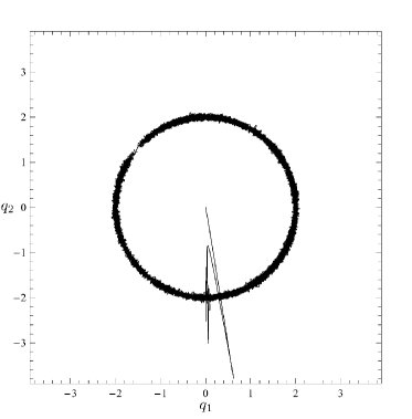
Figure 1: Two dimensional motion of an active particle under the influence of harmonic forces in the $q_{1,}q_{2}$-plane, subject to equations (9)-(11) with all parameters chosen to be equal to one except $d_{1}=5$ and $s^{\frac{1}{2}}=0.3$. The radius of the circle can be calculated from equation (23): $r_{0}=2$. Initial conditions are $q_{1}(0)=0=q_{2}(0),\,p_{1}(0)=0=p_{2}(0),\,e(0)=0$.

Out of its initial conditions, the particle drops onto a circle and then diffuses in no preferred direction, until the whole ring area is filled with trajectories. This random motion on a ring can be explained by referring to the structure of the effective potential, which for the harmonic example reads

$$\tilde{U}(r)=ar^{2}-\frac{d_{1}c_{1}}{c_{3}}\ln\left(c_{2}+c_{3}ar^{2}\right)$$ (22)

in terms of the radial coordinate $r=\left(q_{1}{}^{2}+q_{2}{}^{2}\right)^{\frac{1}{2}}$. The minima of $\tilde{U}(r)$ are found to be at all radial distances

$$r_{0}=\left(\frac{d_{1}c_{1}-c_{2}}{ac_{3}}\right)^{\frac{1}{2}},$$ (23)

which is exactly the radius of the circle seen in Figure 1. In the case of no coupling to an internal energy ($d_{1}=0$), the particle would directly fall into the minimum of the external potential (which is at $r=0$), and no diffusion in any direction would be present. Positive values of $r_{0}$ can be realized for critical values of the coupling parameter $d_{1}$, namely if $d_{1}>\frac{c_{2}}{c_{1}}$. Active Brownian particles with a coupling of $e$ to the potential energy feel a different landscape than the prescribed one, i.e. an effective environment, which is then searched for minimum areas. The internal energy effect in our present example results in trapping the particle not at the origin, but on a circle of a given radius $r=r_{0}$. This stationary state of noise-induced wandering in the valley of minima is immediately present after the internal energy has finally relaxed to its constant value $e_{0}$, given by equation (13). In the minimum region $r=r_{0}$, so the stationary value of the internal energy can be calculated directly:

$$e_{0}=\frac{c_{1}}{c_{2}+c_{3}ar_{0}{}^{2}}=\frac{1}{d_{1}}.$$ (24)

Figure 2 shows the relaxation of $e$ to the stationary value $e_{0}$. After initial oscillations it equilibrates to a constant value (which is then slightly disturbed by the noise influences).

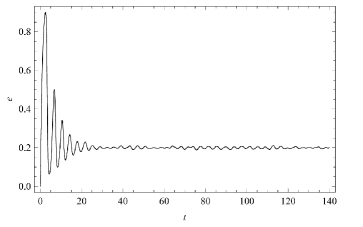
Figure 2: Internal energy evolution in time corresponding to the parameter setup given in Figure 1. The stationary value of $e$ can be calculated from equation (24): $e_{0}=1/5$.

Another remarkable feature of coupling the internal energy to the potential is that equilibrium distributions can be calculated exactly. The standard form of stochastic differential equations (14) & (15) has the following well-known stationary solution of the corresponding Fokker Planck equation:

$$\rho(q,p)\sim e^{-\tilde{H}(q,p)},$$ (25)

which reduces to $\rho(q)\sim e^{-\tilde{U}(q)}$ for the distribution in configuration space, after performing the Gaussian momentum integral. This is an exact equilibrium solution of our nonlinear stochastic process. Former models of active Brownian motion had to rely on specific approximation methods, when studying equilibrium solutions of the corresponding Fokker Planck equation key-7 .

IV Canonical active Brownian motion: Coupling of $e$ to the total mechanical energy

Combining the so far separately imposed couplings to the kinetic, resp. the potential energy, stochastic dynamics are in full generality:

$$\frac{dq_{i}}{dt}=\frac{\partial H}{\partial p_{i}}$$ (26)

$$\frac{dp_{i}}{dt}=-f(e)\frac{\partial H}{\partial q_{i}}-g(e)\frac{\partial H}{\partial p_{i}}+\eta_{i}$$ (27)

$$\frac{de}{dt}=c_{1}-c_{2}e-c_{3}eH$$ (28)

with $H(q,p)=\frac{p^{2}}{2}+U(q)$ and $f(e)=1-d_{1}e$ , $g(e)=\gamma_{0}-d_{2}e$. Recently another generalized model for internal energy dynamics was introduced by Zhang et. al. Zh16 . Whereas in their paper the coupling of internal energy to position and velocity is generated via an arbitrary function of $q$ and $p$, our coupling mechanism is motivated from the idea of exchange between internal and the full mechanical energy. The time differential of the Hamiltonian in the deterministic case reads

$$\frac{dH}{dt}=-g(e)\left(\frac{\partial H}{\partial\mathbf{p}}\right)^{2}+d_{1}e\frac{\partial H}{\partial\mathbf{q}}\frac{\partial H}{\partial\mathbf{p}}=-\gamma_{0}p^{2}+d_{2}ep^{2}+d_{1}e\frac{dU}{dt}.$$ (29)

If the internal energy equilibrates after some time, its stationary value would be

$$e(H)=\frac{c_{1}}{c_{2}+c_{3}H},$$ (30)

so that dynamics reduce to

$$\frac{dq_{i}}{dt}=\frac{\partial H}{\partial p_{i}}$$ (31)

$$\frac{dp_{i}}{dt}=-F(H)\frac{\partial H}{\partial q_{i}}-G(H)\frac{\partial H}{\partial p_{i}}+\eta_{i}$$ (32)

with the two dissipation functions

$$F(H)=1-\frac{d_{1}c_{1}}{c_{2}+c_{3}H}\quad,\quad G(H)=\gamma_{0}-\frac{d_{2}c_{1}}{c_{2}+c_{3}H}.$$ (33)

Stochastic equations for active Brownian motion now truly define a canonical system, in the sense that all parts of the dynamics are completely given by the Hamiltonian function, which was not the case for separate couplings to $\frac{p^{2}}{2}$ or $U(q)$. Only when we consider free particles ($H=\frac{p^{2}}{2}$), so that in equation (8) $\gamma(p^{2})=\gamma(H)$, active Brownian motion in its original sense is a canonical system. When coupling the internal energy to the Hamiltonian, also the general case of active Brownian particles with interactions (i.e. with a potential) represents a canonical dissipative system. The method of coupling $e$ to the full mechanical energy leads to a novel type of canonical dissipative system, which has a more complex dissipative behavior and is more general than those ones which currently exist in the literature mycitation ; toda ; qgases .

V Bifurcations of Equilibria

In this section, we investigate equilibrium solutions of canonical active Brownian motion and its possible bifurcation scenarios. Bifurcation theory studies the qualitative change of solutions for a dynamical system when parameters are varied. Static bifurcations are present, e.g., when for some critical parameter values, two equilibrium points become stable while another one loses its stability. Apart from dealing only with stationary solutions, dynamic bifurcations describe how equilibrium points can bifurcate into nonequilibrium orbits, e.g. limit cycles. We will encounter both of these bifurcation scenarios in canonical active Brownian motion. Special attention is given to nonequilibrium solutions, i.e. situations in which $\frac{de}{dt}\neq 0$. Bifurcations of active Brownian motion for some special case of generalized internal energy dynamics were studied also in Zh16 . However, no bifurcation analysis for velocity and space dependent internal energy equations were given, nor was considered the case of an external harmonic potential. We will investigate the non-equilibrium behavior of active Brownian motion, when both kinetic and potential energy coupling is present.

For the following explicit calculations, we assume the harmonic external potential $U(q)=\frac{1}{2}q^{2}$. Stochastic differential equations (26)-(28) then read

$$\frac{dq_{i}}{dt}=p_{i}\quad,\quad\frac{dp_{i}}{dt}=-(1-d_{1}e)q_{i}-(\gamma_{0}-d_{2}e)p_{i}+\eta_{i}$$ (34)

$$\frac{de}{dt}=c_{1}-c_{2}e-c_{3}e\frac{p^{2}}{2}-c_{4}e\frac{q^{2}}{2},$$ (35)

where we have separated the couplings of $e$ to the kinetic and the potential energy for later analysis of special cases.

V.1 One Dimension

Equilibria in one dimension for the deterministic case are

$$q_{0}=0=p_{0},\quad e_{0}=\frac{c_{1}}{c_{2}}$$ (e1)

$$q_{0}=\pm\left\{\frac{2(d_{1}c_{1}-c_{2})}{c_{4}}\right\}^{1/2},\quad p_{0}=0,\quad e_{0}=\frac{1}{d_{1}}$$ (e2)

Stability conditions of these points are obtained by linearizing the system. In equations (34) & (35), we make the shift $q\rightarrow q+q_{0}$, $p\rightarrow p+p_{0}$, $e\rightarrow e+e_{0}$, neglecting any terms of order higher than one. Then dynamics are given only by the Jacobian matrix, whose eigenvalues can be studied for each of the three equilibria separately. For equilibrium (e1), the eigenvalues of the Jacobian are

$$\lambda_{1}=-c_{2}\quad,\quad\lambda_{2,3}=-\frac{\gamma_{0}-\frac{d_{2}c_{1}}{c_{2}}}{2}\pm\left\{\left(\frac{\gamma_{0}-\frac{d_{2}c_{1}}{c_{2}}}{2}\right)^{2}+\frac{d_{1}c_{1}}{c_{2}}-1\right\}^{\frac{1}{2}}.$$ (36)

The real parts of all $\lambda_{i}$’s are negative if $\gamma_{0}c_{2}>d_{2}c_{1}$ and $c_{2}>d_{1}c_{1}$. Hence, equilibrium (e1) remains stable as long as these two conditions are fulfilled. Figure 3 shows a trajectory in phase space $(q,p,e)$ approaching equilibrium (e1).

The corresponding eigenvalues for equilibria (e2) are not accessible so easily, so we follow the Routh-Hurwitz theorem key-8 , which allows one to calculate stability regions by analyzing only the characteristic equation of the Jacobian, without any need for solving it. Application of this scheme for equilibria (e2) results in the conditions $\gamma_{0}d_{1}>d_{2},\,c_{2}<d_{1}c_{1}$ and $(\gamma_{0}d_{1}-d_{2})(c_{1}^{2}d_{1}^{2}+c_{1}(\gamma_{0}d_{1}-d_{2}))>2d_{1}(c_{1}d_{1}-c_{2})$ for both of them.

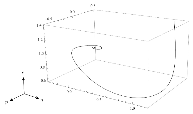
Figure 3: Trajectory to equilibrium (e1), parameters satisfying the corresponding stability conditions: $\gamma_{0}=1$, $c_{1}=1$, $c_{2}=2$, $c_{3}=2$, $c_{4}=2$, $d_{1}=1$, $d_{2}=1$. (The internal energy is plotted with a factor of 2.)

Two types of bifurcations can be seen, a static and a dynamic one. First we observe a Pitchfork-bifurcation of equilibrium (e1) into the two other ones at $c_{2}=d_{1}c_{1}$: As long as $c_{2}>d_{1}c_{1}$ is fulfilled, equilibrium (e1) is stable, while equilibria (e2) do not exist. For parameter regions where $c_{2}<d_{1}c_{1}$, equilibria (e2) are stable, while equilibrium (e1) becomes unstable. Apart from this static bifurcation we observe a dynamic bifurcation, namely a Hopf-bifurcation, at $\gamma_{0}c_{2}=d_{2}c_{1}$: Suppose we fix the condition $c_{2}>d_{1}c_{1}$, by looking at the eigenvalues (36), we see the appearance of a purely imaginary pair of eigenvalues $\lambda_{2,3}=\pm i\omega$ at the critical point $\gamma_{0}c_{2}=d_{2}c_{1}$ (while $\mathrm{Re}\lambda_{1}\neq 0$). This is the general condition for the existence of a Hopf-bifurcation, which describes equilibria bifurcating into periodic solutions key-9 . Equilibrium (e1) bifurcates into limit cycles at the Hopf bifurcation point $\gamma_{0}c_{2}=d_{2}c_{1}$. One example of these limit cycles is shown in figure 4.

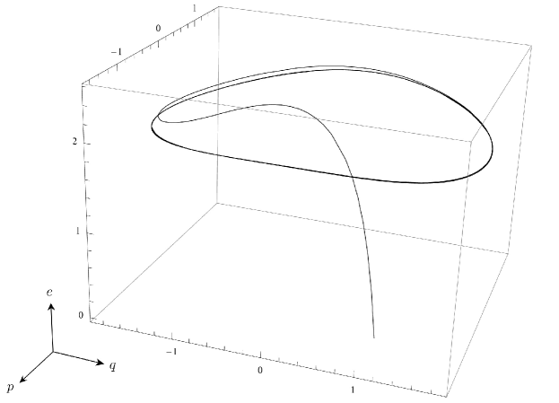
Figure 4: Limit cycle appearing after the Hopf-bifurcation point. Parameter values are: $\gamma_{0}=1$, $c_{1}=1$, $c_{2}=2$, $c_{3}=2=c_{4}$, $d_{1}=1$, $d_{2}=5$. Initial conditions were chosen to be $q(0)=0$, $p(0)=-1$ and $e(0)=0$. (The internal energy is plotted with a factor of 10.)

V.2 Arbitrary Dimensions

A similar study can be made for arbitrary dimensions $n$. First we reduce the $(2n+1)$-dimensional system (34) & (35) to four dimensions by transforming to the variables $K=\frac{p^{2}}{2}$, $U=\frac{q^{2}}{2}$ and $S=\mathbf{qp}$. Evolution equations in its deterministic form therefore transform to

$$\frac{dK}{dt}=-2(\gamma_{0}-d_{2}e)K-(1-d_{1}e)S\quad,\quad\frac{dU}{dt}=S$$ (37)

$$\frac{dS}{dt}=2K-(\gamma_{0}-d_{2}e)S-2(1-d_{1}e)U,$$ (38)

$$\frac{de}{dt}=c_{1}-c_{2}e-c_{3}eK-c_{4}eU.$$ (39)

The following are the three possible equilibrium points:

$$S_{0}=K_{0}=U_{0}=0,\quad e_{0}=\frac{c_{1}}{c_{2}}$$ (E1)

$$S_{0}=K_{0}=0,\quad U_{0}=\frac{c_{1}d_{1}-c_{2}}{c_{4}},\quad e_{0}=\frac{1}{d_{1}}$$ (E2)

$$S_{0}=0,\quad K_{0}=\left(1-\frac{d_{1}\gamma_{0}}{d_{2}}\right)U_{0},\quad U_{0}=\frac{d_{2}c_{1}-c_{2}\gamma_{0}}{\gamma_{0}c_{3}\left(1-\frac{d_{1}\gamma_{0}}{d_{2}}\right)+\gamma_{0}c_{4}},\quad e_{0}=\frac{\gamma_{0}}{d_{2}}.$$ (E3)

Before addressing bifurcation theory, we shortly comment on how these equilibrium points of canonical active Brownian motion contain equilibria of the separately coupled versions. The equilibrium solution of original active Brownian motion (coupling of $e$ only to the kinetic energy) for a harmonic potential key-2 is identical to the equilibrium point (E3), if $d_{1}=0$ and $c_{4}=0$. The case of internal energy coupling only to the potential, studied in Section III, is identical to equilibrium (E3), also for nonvanishing $d_{2}$ and $c_{3}$. Active Brownian motion in its fully coupled form therefore shares the same equilibrium solution with the system when coupled only to the potential. Therefore the same trajectories as already shown in figure 1 can be seen.

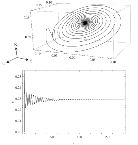
Figure 5: Trajectory in 4-dimensional phase space to equilibrium (E3) for the following choice of parameters: $\gamma_{0}=11$, $c_{1}=4$, $c_{2}=0.01$, $c_{3}=129$, $c_{4}=31$, $d_{1}=0.01$, $d_{2}=48$ and initial conditions $S(0)=0.1$, $U(0)=0.1$, $K(0)=0.1$, $e(0)=0.2$. (The kinetic energy $K$ is plotted with a factor of 3.)

We now repeat our linearization procedure concerning stability properties and bifurcations. Eigenvalues of the Jacobian associated with equilibrium (E1) can be calculated straightforwardly:

$$\lambda_{1}=-c_{2}\quad,\quad\lambda_{2}=\frac{c_{1}d_{2}-c_{2}\gamma_{0}}{c_{2}}$$ (40)

$$\lambda_{3,4}=\frac{c_{1}d_{2}-c_{2}\gamma_{0}}{c_{2}}\pm\left\{\left(\gamma_{0}-\frac{d_{2}c_{1}}{c_{2}}\right)^{2}+4\left(\frac{d_{1}c_{1}}{c_{2}}-1\right)\right\}^{\frac{1}{2}}.$$ (41)

The real parts are negative if the conditions $\gamma_{0}c_{2}>d_{2}c_{1}$ and $c_{2}>d_{1}c_{1}$ are fulfilled (these are the same conditions as for equilibrium (e1) in one dimension). The stability analysis for equilibrium (E2) can be carried out via the Routh-Hurwitz theorem and it leads to the same conditions as for equilibrium (e2) in one dimension. Equilibrium (E3) is hard to analyze even with the Routh-Hurwitz procedure, so that we have no information about stability regions for this third stationary solution at all. Nonetheless we are able to find parameter values by hand which lead to trajectories approaching it slowly, as is shown in Figure 5. Concerning the bifurcation behavior of our system, we observe two collisions of equilibria at critical parameter values of $d_{2}$ (which we choose as our bifurcation parameter in the following).

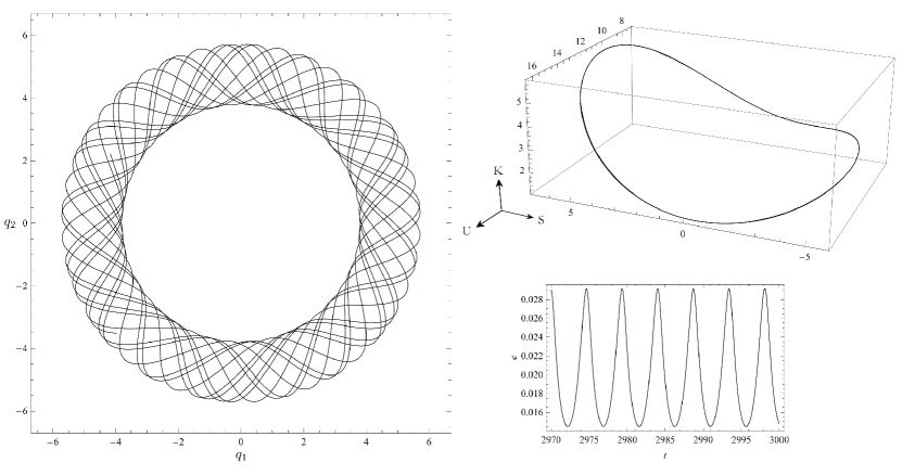
Figure 6: Limit cycle in the phase space of variables $(K,U,S,e)$ and its corresponding quasi-periodic motion in configuration space for $n=2$ after the transient phase. Parameter values are $\gamma_{0}=1$, $c_{1}=1$, $c_{2}=2$, $c_{3}=4$, $c_{4}=4$, $d_{1}=49$, $d_{2}=50$ and initial conditions $S(0)=0$, $U(0)=0$, $K(0)=1$, $e(0)=0$. Corresponding initial conditions in $(q_{i},p_{i},e)$: $q_{1}(0)=0=q_{2}(0)$, $p_{1}(0)=-1=p_{2}(0)$, $e(0)=0$. (The kinetic energy $K$ is plotted with a factor of 3.)

Such collisions are usually associated with Fold-bifurcations. Its general property is the existence of a simple zero eigenvalue of the Jacobian. This happens for equilibrium (E1) when $d_{2}=\frac{c_{2}\gamma_{0}}{c_{1}}$, so that $\lambda_{2}$ vanishes. At the Fold-bifurcation point $d_{2}=\frac{c_{2}\gamma_{0}}{c_{1}}$, equilibrium (E1) becomes identical with equilibrium (E3). Before the bifurcation, when $d_{2}<\frac{c_{2}\gamma_{0}}{c_{1}}$, equilibrium (E1) is stable, while (E3) does not exist, since the potential $U=\frac{1}{2}q^{2}$ has to be positive. After the Fold-point, when $d_{2}>\frac{c_{2}\gamma_{0}}{c_{1}}$, equilibrium (E1) is unstable, and (E3) is observed to be stable (see Figure 5 for one example).

Another Fold-bifurcation is present at $d_{2}=\gamma_{0}d_{1}$, which is a bifurcation of equilibrium (E2). Although three of its eigenvalues are not accessible in a treatable way, one of them is in a simple form, namely $\lambda=\frac{2(d_{2}-d_{1}\gamma_{0})}{d_{1}}$. It vanishes for $d_{2}=\gamma_{0}d_{1}$ and we see the collision of equilibrium (E2) with (E3) at this point. Before this critical value, when $d_{2}<\gamma_{0}d_{1}$, equilibrium (E2) is stable, while (E3) does not exist, since the kinetic energy $K=\frac{1}{2}p^{2}$ has to be positive. After the bifurcation point, when $d_{2}>\gamma_{0}d_{1}$, equilibrium (E2) is unstable, while (E3) can be observed to be stable (see again Figure 5).

Apart from these two collisions of equilibria, a Fold-Hopf bifurcation is present. Remember that in one dimension we observed a Hopf bifurcation at some critical point in parameter space. In arbitrary dimensions, if the condition $c_{2}>d_{1}c_{1}$ is fulfilled, the eigenvalues $\lambda_{3,4}$ of equilibrium (E1) become a purely conjugate complex pair $\lambda_{3,4}=\pm i\omega$ at $d_{2}=\frac{\gamma_{0}c_{2}}{c_{1!}}$ and $\lambda_{2}$ vanishes exactly. This zero-pair constellation at some critical point in parameter space is the general condition for a Fold-Hopf-bifurcation. To this type of bifurcation are associated various non-equilibrium dynamics, ranging from motions on tori to heteroclinic orbits key-9 . We do not want to address the analysis of this Fold-Hopf-bifurcation here, instead focusing on the interesting case, when stable limit cycles are present in our 4-dimensional system. Figure 6 shows a limit cycle in phase space $(K,U,S,e)$. This periodic motion corresponds to a quasi-periodic motion in configuration space, as is shown for $n=2$. Adding noise to our system doesn’t change the qualitative behavior, only the direction of movement can change at some instances.

Concluding this analysis of non-equilibrium behavior, we want to emphasize the various possibilities that arise from studying parameter regions where $e$ is not constant, but heavily oscillating. Far away from stationary solutions, our system shows to have quasi-periodic dynamics.

VI Synopsis and Outlook

We have formulated a generalized version of active Brownian motion in the sense that we allow not only couplings of the internal energy to the kinetic energy, but also to the potential energy and more generally to the Hamiltonian. The latter case gives rise to a canonical dissipative system. Analysis of stationary points and its possible bifurcations into non-equilibrium solutions reveals a rich dynamical structure in parameter regions far away from equilibrium. Explicit numerical studies of all bifurcation scenarios will be left to future computer art; nevertheless we were able to find interesting quasi-periodic dynamics by hand. The various non-equilibrium phenomena may be relevant in future applications to real systems, which do not rely on the assumption of stationary internal energies. Moreover, many particle systems with mutual interactions can be studied within the scheme of canonical active Brownian motion. The self-organizing properties e.g. of swarms will be of special interest for upcoming papers, when applying our model for a system composed of many particles.

- (1) C. W. Gardiner: Handbook of stochastic methods, 3rd. ed., Springer, Berlin 2004.
- (2) F. Schweitzer, W. Ebeling, B. Tilch: Complex motion of Brownian particles with energy depots, Phys. Rev. Lett. 80 (23), 5044-5047 (1998).
- (3) U. Erdmann, W. Ebeling, L. Schimansky-Geier, F. Schweitzer: Brownian particles far from equilibrium, Eur. Phys. J. B 15, 105-113 (2000).
- (4) L. Schimansky-Geier, W. Ebeling, U. Erdmann: Stationary distribution densities of active Brownian particles, Act. Phys. Pol. B 36 (5), 1757-1769 (2005).
- (5) F. Schweitzer: Brownian agents and active particles, Springer, Berlin 2003.
- (6) W. Ebeling, F. Schweitzer, B. Tilch: Active Brownian particles with energy depots modelling animal mobility, BioSystems 49, 17-29 (1999).
- (7) F. Schweitzer, W. Ebeling, B. Tilch: Statistical mechanics of canonical-dissipative systems and applications to swarm dynamics, Phys. Rev. E 64, 02110/1-12 (2001).
- (8) W. Ebeling, F. Schweitzer: Swarms of particle agents with harmonic interactions, Th. Biosc. 120/3-4, 207-224 (2001).
- (9) R. Mach, F. Schweitzer: Modeling vortex swarming in Daphnia, Bull. Math. Biol. 69, 539-562 (2007).
- (10) A. Glück, H. Hüffel: Nonlinear Brownian motion and Higgs mechanism, Phys. Lett. B 659, 447-451 (2008).
- (11) M. L. Deng, W. Q. Zhu: Stationary motion of active Brownian particles, Phys. Rev. E 69, 046105/1-9 (2004).
- (12) V. A. Makarov, W. Ebeling, M. G. Velarde: Solition-like waves on dissipative Toda lattices, Int. J. Bif. & Chaos 10 (5), 1075-1089 (2000).
- (13) W. Ebeling: Canonical nonequilibrium statistics and applications to Fermi-Bose systems, Cond. Matter Phys. 3 (2/22), 285-293 (2000).
- (14) DeJesus E. X., Kaufman Ch.: Routh-Hurwitz criterion in the examination of eigenvalues of a system of nonlinear ordinary differential equations, Phys. Rev. A 35 (12), 5288-5290 (1987).
- (15) Kuznetsov, Yuri A.: Elements of applied Bifurcation Theory, Springer, New York 1995.
- (16) Y. Zhang, C. K. Kim, K.-J.-B. Lee: Active motions of Brownian particles in a generelized energy-depot model, New J. Phys. 10, 103018 (2008).
- (17) W. Ebeling, U. Erdmann, J. Dunkel, M. Jenssen: Nonlinear Dynamics and Fluctuations of Dissipative Toda Chains, J. Stat. Phys. 101, 443-457 (2000).
- (18) A. P. Chetverikov, W. Ebeling, M. G. Velarde: Thermodynamics and phase transitions in dissipative and active Morse chains, Eur. Phys. J. B 44, 509-519 (2005).