Evolution of density perturbations in decaying vacuum cosmology: The case of non-zero perturbations in the cosmological term

Abstract

We extend the results of a previous paper where a model of interacting dark energy, with a cosmological term decaying linearly with the Hubble parameter, is tested against the observed mass power spectrum. In spite of the agreement with observations of type Ia supernovas, baryonic acoustic oscillations and the cosmic microwave background, we had shown previously that no good concordance is achieved if we include the mass power spectrum. However, our analysis was based on the ad hoc assumption that the interacting cosmological term is strictly homogeneous. Now we perform a more complete analysis, by perturbing such a term. Although our conclusions are still based on a particular, scale invariant choice of the primordial spectrum of dark energy perturbations, we show that a cosmological term decaying linearly with the Hubble parameter is indeed disfavored as compared to the standard model.

I Introduction

The elucidation of the nature of dark energy is one of the most important challenges of modern cosmology, requiring at present the attention of theoreticians and observational teams. From the theoretical viewpoint, a crucial problem is to understand the role of vacuum in the cosmological scenario, its possible relation with dark energy and, in this case, why its observed density is so small as compared to the value theoretically expected by quantum field theories Pad .

Among the different approaches to this problem, one can find the suggestion that dark energy is the manifestation of quantum vacuum in the curved space-time, and that its density depends on the curvature, decaying from a huge initial value as space expands. As the total energy must be conserved, the vacuum decay is concomitant with matter production, a general feature of this kind of models and, more generally, of interacting dark energy models Ozer ; Horvat ; SC ; Grande ; Holografia ; Zimdahl ; Ma ; Fabris .

However, it is difficult to derive the vacuum contribution in the expanding background, and some phenomenological approaches are needed in order to implement the above idea. A thermodynamical analysis in de Sitter space-time, in line with the holographic conjecture, has suggested a particular dependence of the vacuum density $\Lambda$ on the Hubble parameter $H$, which is a good approximation in expanding, quasi-de Sitter space-times SC2 .

Such a dependence was obtained by noting that a free particle in the de Sitter background presents, superposed to its normal modes, a thermal motion with a characteristic temperature equals to $H$, which is an expression of the known association of a temperature $H$ to the de Sitter horizon. On the other hand, if we regularize the vacuum energy density in the flat space-time by postulating a thermal distribution of the vacuum fluctuation modes at a temperature $m$ (which is equivalent to impose a superior cutoff $m$ on the modes frequencies), we obtain $\Lambda_{0}\approx m^{4}$. Now, if in de Sitter space-time we shift this vacuum temperature from $m$ to $m+H$ we obtain, after subtracting the flat space-time contribution, the ansatz $\Lambda\approx(m+H)^{4}-m^{4}$.

This is a phenomenological ansatz, in the sense that there is still no rigorous derivation of it in the realm of quantum field theories in curved space-time. Other interesting ansatzen have been proposed as well, also on phenomenological or semi-phenomenological basis (see, for example, Grande ; Holografia ; Fabris ). In this context the comparison with observations is relevant, since it can rule out or constrain some models while we do not have a rigorous theoretical answer to the problem.

If we use for the cutoff $m$ the energy scale of the QCD phase transition (the latest known cosmological vacuum transition), in the limit of very early times we have $H>>m$, and the cosmological term is proportional to $H^{4}$. This leads to a non-singular inflationary solution, with an initial quasi-de Sitter phase giving origin to a radiation-dominated universe, with a matter content generated at the expenses of vacuum energy SC2 .

For late times all depends on the masses of the produced particles. The time-energy uncertainty relation suggests that particles of mass $M$ can only be produced if $H>M$. Hence, massive particles as the baryonic matter, axions and supersymmetric candidates for dark matter should stop to be produced at the time of electro-weak phase transition (whereas the production of photons and massless neutrinos must be forbidden by some selection rule, otherwise our universe would be completely different at present). Therefore, if no other particle is taken into account, for late times we have a genuine cosmological constant, like in the standard $\Lambda$CDM model. However, if we consider the possibility of very light dark particles (as massive gravitons, for example), the vacuum decay could still happen. Since in this limit we have $H<<m$, now the vacuum density varies linearly with $H$, that is, $\Lambda\approx m^{3}H$ SC2 . On the other hand, as in the present universe the cosmological term is dominant, the Friedmann equation gives $\Lambda\approx H^{2}$. Hence, we have $H\approx m^{3}$ and $\Lambda\approx m^{6}$. With $m$ of the order of the energy scale of the QCD chiral phase transition (approximately the pion mass), these expressions lead to numerical coincidences (in orders of magnitude) with the observed current values of $H$ and $\Lambda$.

In this case, the resulting scenario is similar to the standard one, with the radiation phase followed by a long matter era, with the cosmological term dominating for large times Borges . A detailed analysis of the redshift-distance relation for type Ia supernovas, the baryonic acoustic oscillations (BAO) and the position of the first peak in the spectrum of anisotropies of the cosmic microwave background (CMB) has shown a very good concordance Jailson2 , with present values for the Hubble parameter, the relative matter density and the universe age inside the limits imposed by other, non-cosmological observations.

Nevertheless, a late-time matter production may dilute the density contrast during the process of structure formation Reuven . Therefore, the study of the evolution of perturbations and the comparison of the model predictions with the observed mass power spectrum is also necessary. In a previous paper I we have shown that, in the case of a strictly homogeneous cosmological term (which means that matter production is homogeneous as well), the matter contrast is indeed suppressed at late times, after achieving a maximum near the present epoch. This would be a potential explanation for the cosmic coincidence, but it also leads to a suppression in the power spectrum. As a consequence, a good accordance with observations is only possible with a relative matter density above the concordance value obtained from the joint analysis of supernovas, BAO and CMB.

This would rule out the late-time vacuum decay in the context of the present model, but the homogeneity of the interacting cosmological term is an ad hoc hypothesis, which should be relaxed before taking a definite conclusion. If matter is perturbed, the interacting dark energy must also be, and we have to verify whether such a perturbation is negligible or not. That is what we do in the present paper. By writing our ansatz for the variation of vacuum density in a covariant form, we derive a natural expression for the linear perturbations in the cosmological term, which can be integrated together with the relativistic equations for perturbations in matter and radiation. We then construct the predicted mass power spectrum, comparing with the observational data. Our conclusion is that, assuming a scale invariant primordial spectrum for the vacuum perturbations, a late-time vacuum decay linear with $H$ is clearly ruled out also in this case.

The paper is organized as follows. In the next section we briefly review the main features of the present model and its accordance with other kind of observations. In Section III we obtain and integrate the set of coupled perturbations equations for the vacuum, matter, radiation and metric, obtaining the corresponding power spectrum. In Section IV we outline our conclusions.

II The model

There are two main motivations to consider that $\Lambda$ should vary with time. The first one concerns the theoretically predicted value for the cosmological constant, seen as a manifestation of vacuum energy, and its observational value, a discrepancy that mounts to 120 orders of magnitude. Considering some special ingredients, like supersymmetry, this discrepancy can be reduced to about 60 orders of magnitude, what is still a huge value. In view of this problem, it would be interesting to have a mechanism that could reduce the value of $\Lambda$, in order it could fill its role in the inflationary era, attaining later its present, small value. This could be achieved by allowing $\Lambda$ to vary with time. The second motivation concerns the coincidence problem: the observed value of the cosmological constant is of the same order of magnitude of the ordinary matter density. Since the energy density of $\Lambda$ is, in principle, constant and the energy density of ordinary matter varies with time, this equivalence can only be obtained in a given moment in the history of the evolution of the universe. It is quite remarkable that this occurs exactly today, when the process of galaxy formation is already essentially finished. If we do not want to invoke a rather controversial principle, like the anthropic one, it would be necessary to obtain a mechanism that generate this fact. Giving dynamics to $\Lambda$ is a natural approach to this coincidence problem. In any case, due to energy conservation, the variation in time is equivalent to allow $\Lambda$ to decay, generating matter, for example.

The decay of $\Lambda$ into matter may solve the problems described above and, at the same time, may somehow explain the origin of dark matter. How to achieve such decaying process? The most simple idea is to consider the conservation law

$$\dot{\rho}+3\frac{\dot{a}}{a}(\rho+p)=0,$$ (1)

and suppose that $\rho=\rho_{m}+\rho_{\Lambda}$ and $p=p_{m}+p_{\Lambda}$, where $m$ stands for matter. Imposing now that $p_{m}=0$ and $p_{\Lambda}=-\rho_{\Lambda}$, the above conservation equation becomes

$$\dot{\rho}_{m}+3\frac{\dot{a}}{a}\rho_{m}=-\dot{\rho}_{\Lambda}.$$ (2)

As far as $\rho_{\Lambda}$ decays ($\dot{\rho}_{\Lambda}<0$), the energy density of the cosmological constant is converted into matter.

This simple phenomenological approach faces a major drawback: In doing so, we remain with the same number of equations, but we have added a new function to be determined. Hence, we need an expression which says how $\Lambda$ decay. One possibility is to invoke the holographic principle. It says that the physical content of a given system, defined in a volume $V$, is encoded in the area of the surface enveloping this volume, $A$. This principle is motivated by the black-hole thermodynamics: the entropy of a black-hole is given just by the area of the event horizon, $S_{BH}=\frac{A}{4}$. Another motivation, somehow related to the previous one, is given by the AdS/CFT correspondence. For a review, see bousso . In cosmology, the problem can be addressed by establishing a connection between the infrared and the ultraviolate cut-off defined in the universe. The ultraviolet cut-off may be given, for example, by the Planck’s length, while the infrared cut-off is usually given by the Hubble’s radius. Since the Hubble radius is a function of time, $\Lambda$ becomes a function of time. In reference Holografia the holographic principle is used in order to give dynamics to $\Lambda$, but exploiting also the possibility that the infrared cut-off is given by the particle horizon or the future event horizon, besides the Hubble radius. In this way the authors conclude that $\Lambda$ should behave as the square of the Hubble function, and not linearly as for our model. The use of different infrared cut-offs in Holografia leads to different effective equations of state for the mixture matter-$\Lambda$.

Another possibility to determine the time variation of $\Lambda$ is to consider quantum effects due to matter fields in the universe. In this case, $\Lambda$ can be seen as a running parameter: the renormalization group related to quantum fields in the dynamic background of the FRW space-time implies that $\Lambda$ must run, that is, must vary with time. In reference shapiro (see also Fabris ) this mechanism has been investigated and the authors found that $\Lambda$ must behave generally as $\Lambda=\Lambda_{0}+\sigma H^{2}$, where $\Lambda_{0}$ is a constant and $\sigma$ is a parameter which depends on the ratio of the mass of the quantum fields with respect to Planck’s mass, and on their nature (fermions or bosons). This approach is quite distinct from the approach of the present paper and from that of reference Holografia , since it is based on the effective action due to quantum effects in the universe. A variation of such model is the so-called $\Lambda XCDM$ model Grande , where the cosmological term is supposed to interact with a new field, called cosmon, which has an equation of state $p_{X}=\omega_{X}\rho_{X}$.

There is in the literature a large number of proposals leading to a varying cosmological term. For some other frameworks, see boussobis . We will return later to the constraints due to the LSS observational test on the models described above. Now, let us describe in more details the model studied in this paper.

In the presence of pressureless matter and a time-dependent cosmological term, the Friedmann equations in the spatially flat case can be written as (we are using $8\pi G=c=1$)

$$\dot{\rho}_{m}+3H\rho_{m}=-\dot{\Lambda},$$ (3)

$$\rho_{m}+\Lambda=3H^{2},$$ (4)

where the dot means derivative with respect to the cosmological time $t$, and $\rho_{m}$ is the matter density.

Let us take our late-time ansatz $\Lambda=\sigma H$, with $\sigma$ constant and positive. From the above equations we obtain the evolution equation

$$2\dot{H}+3H^{2}-\sigma H=0.$$ (5)

The solution, for $\rho_{m},H>0$, is given by Borges

$$a=C\left[\exp\left(\sigma t/2\right)-1\right]^{2/3},$$ (6)

where $a$ is the scale factor and $C$ is an integration constant (another integration constant was taken equal to zero in order to have $a=0$ for $t=0$). Taking the limit of early times, we have $a\propto t^{2/3}$, as in the Einstein-de Sitter solution. It is also easy to see that, in the opposite limit $t\rightarrow\infty$, (6) tends to the de Sitter solution.

With the help of (6), and by using $\Lambda=\sigma H$ and $\rho_{m}=3H^{2}-\sigma H$, it is straightforward to derive the matter and vacuum densities as functions of the scale factor. One has

$$\rho_{m}=\frac{\sigma^{2}C^{3}}{3a^{3}}+\frac{\sigma^{2}C^{3/2}}{3a^{3/2}},$$ (7)

$$\Lambda=\frac{\sigma^{2}}{3}+\frac{\sigma^{2}C^{3/2}}{3a^{3/2}}.$$ (8)

In these expressions, the first terms give the standard scaling of matter (baryons included) and vacuum densities, being dominant in the limits of early and very late times, respectively. The second ones are owing to the process of matter production, being important at an intermediate time scale.

From (6) we can also derive the Hubble parameter as a function of time. It is given by

$$H=\frac{\sigma/3}{1-\exp(-\sigma t/2)}.$$ (9)

Finally, with the help of (6) and (9) we can express $H$ as a function of the redshift $z$, which leads to

$$H(z)=H_{0}\left[1-\Omega_{m0}+\Omega_{m0}(z+1)^{3/2}\right].$$ (10)

Here, $\Omega_{m0}\equiv\rho_{m0}/(3H_{0}^{2})$ and $H_{0}$ are the present values of the relative matter density and Hubble parameter, respectively.

Note that expression (10) is valid only for late times, when radiation can be neglected. For higher redshifts we need an appropriate extension of it. As discussed in Jailson2 ; I , for times when radiation is important, the cosmological term and the matter production are negligible. Therefore, a very good approximation can be achieved by simply adding a conserved radiation term to the total energy density. In this way we obtain

$$H(z)\approx H_{0}\left\{\left[1-\Omega_{m0}+\Omega_{m0}(1+z)^{3/2}\right]^{2}+\Omega_{R0}(1+z)^{4}\right\}^{1/2},$$ (11)

where $\Omega_{R0}=\rho_{R0}/(3H_{0}^{2})$ is the relative radiation density at present.

We have analysed the redshift-distance relation for type Ia supernovas Jailson2 , obtaining data fits as good as with the spatially flat $\Lambda$CDM model. With the Supernova Legacy Survey (SNLS) SNLS the best fit is given by $h=0.70\pm 0.02$ and $\Omega_{m0}=0.32\pm 0.05$ (with $2\sigma$), with a reduced $\chi$-square $\chi^{2}_{r}=1.01$ (here, $h\equiv H_{0}/$($100$km/s.Mpc)). With the inclusion of baryonic acoustic oscillations in the analysis these results remain practically unaltered. On the other hand, a joint analysis of the Legacy Survey, BAO and the position of the first peak of CMB anisotropies has led to the concordance values $h=0.69\pm 0.01$ and $\Omega_{m0}=0.36\pm 0.01$ (with $2\sigma$), with $\chi^{2}_{r}=1.01$ Jailson2 . Note that the concordance value of $\Omega_{m0}$ is above the current $\Lambda$CDM value sanchez . This is a feature of the present model, and a discussion about its origin can be found in Jailson2 and I .

III The mass power spectrum

As the cosmological term has non-zero pressure, the inclusion of its perturbations requires a relativistic treatment, and the first step is to put the variation law for $\Lambda$ in a covariant form. In comoving observers, it is possible to rewrite our late-time ansatz $\Lambda=\sigma H$ as

$$\Lambda=\frac{\sigma}{3}u^{\nu}_{;\nu},$$ (12)

where $u^{\nu}_{;\nu}$ is the covariant divergence of the cosmic fluid $4$-velocity. Of course, this is not the only option to express the ansatz covariantly. But it seems the most natural and the simplest one.

We can now perturb this ansatz. By defining $\theta=\partial_{i}\delta u^{i}$ and introducing the metric perturbation $h=h_{kk}/a^{2}$, we obtain

$$\delta\Lambda=\frac{\sigma}{3}\left(\theta-\frac{\dot{h}}{2}\right).$$ (13)

The other perturbation equations can be obtained by perturbing the Einstein and the covariant energy conservation equations. This was done in reference I , where we consider conserved radiation, matter and the interacting vacuum term as the energy components. Here we will introduce two basic differences. The first one was already discussed, namely the perturbation of the vacuum component. Secondly, we will consider baryons independently conserved, with a separated continuity equation, since they are not produced as vacuum decays. This second novelty does not lead to important differences in the resulting spectrum, but turns the analysis more precise. We will also consider, as in reference I , baryons decoupled from radiation, a simplification which does not affect very much our results. Indeed, in the case of the standard $\Lambda$CDM model such a simplification leads to a difference about $10\%$ in comparison with the exact analysis winfried . Finally, we will suppose that at any time the produced dark particles have the same velocity field of the pre-existing interacting fluid formed by dark matter and vacuum. This is a reasonable hypothesis, since we are dealing with matter production in the low energy limit at large times.

On this basis it is straightforward to derive, in the synchronous gauge, the set of equations

$$\ddot{h}+2H\dot{h} = \rho_{dm}\delta_{dm}+\rho_{b}\delta_{b}+2\rho_{R}\delta_{R}-2\Lambda\delta_{\Lambda},$$ (14)

$$\dot{\delta}_{R}+\frac{4}{3}\left(\frac{v_{R}}{a}-\frac{\dot{h}}{2}\right) = 0,$$ (15)

$$\dot{v}_{R} = \frac{k^{2}}{4a}\delta_{R},$$ (16)

$$\dot{\delta}_{dm}-\frac{\dot{\Lambda}}{\rho_{dm}}\delta_{dm}+\frac{v_{dm}}{a}-\frac{\dot{h}}{2} = -\frac{\dot{\Lambda}}{\rho_{dm}}\delta_{\Lambda}-\frac{\Lambda}{\rho_{dm}}\dot{\delta}_{\Lambda},$$ (17)

$$\dot{v}_{dm}+\left(\frac{\dot{\rho}_{dm}}{\rho_{dm}}+4H\right)v_{dm} = -\frac{k^{2}\Lambda}{a\rho_{dm}}\delta_{\Lambda},$$ (18)

$$\dot{\delta}_{b}-\frac{\dot{h}}{2} = 0.$$ (19)

In these equations $k$ is the wave number; $\rho_{dm}$ and $\rho_{b}$ are the energy densities of dark matter and baryons, respectively; $\delta_{i}=\delta\rho_{i}/\rho_{i}$ defines the density contrast of each component; $v_{dm}=a\,\theta$ and $v_{R}$ are the peculiar velocities of dark matter and radiation, respectively. As the baryonic component is pressureless and independently conserved, its peculiar velocity remains uncoupled and tends to zero, being then neglected.

Therefore, for a given background, we have a system of six equations with seven variables, that can be reduced to a system of five equations with six variables if we use $\dot{\delta}_{b}=\frac{{\dot{h}}}{2}$ (equation (19)). To solve the resulting system of five equations, it is also necessary to add our previous equation (13). In this way we can, for example, eliminate $v_{dm}$ from the system. Using our background solution (see Section II), changing the independent variable from the cosmological time $t$ (after making it dimensionless by redefining $H_{0}t\rightarrow t$) to the scale factor $a$, and fixing $a_{0}=1$, we finally obtain the system

$$\delta_{b}^{\prime\prime}+\left(\frac{g}{f^{2}}+\frac{2}{a}\right)\delta_{b}^{\prime} = \frac{3}{2f^{2}}\left(2\Omega_{R}\delta_{R}+\Omega_{b}\delta_{b}+\Omega_{m}\delta_{m}-2\Omega_{\Lambda}\delta_{\Lambda}\right),$$ (20)

$$\delta^{\prime}_{R}+\frac{4}{3}\left(\frac{v_{R}}{af}-\delta_{b}^{\prime}\right) = 0,$$ (21)

$$v_{R}^{\prime}-\frac{k^{2}}{4af}\delta_{R} = 0,$$ (22)

$$\delta^{\prime}_{m}-\frac{1}{1+r}\left(r^{\prime}-\frac{3r}{a}\right)\delta_{m} = -\left[\frac{1}{1+r}\left(r^{\prime}-\frac{3r}{a}\right)+\frac{3}{a}\right]\delta_{\Lambda}-r\delta^{\prime}_{\Lambda},$$ (23)

$$\delta^{\prime}_{\Lambda}+\left\{\frac{f^{\prime}}{f}+\left[\frac{1+4r}{(1+r)a}-\frac{r^{\prime}}{1+r}\right]+\frac{k^{2}r}{3af^{2}}\right\} \delta_{\Lambda} =$$ (24)

$$- \frac{a}{3}\left\{\delta_{b}^{\prime\prime}+\left[\frac{f^{\prime}}{f}+\frac{2+5r}{(1+r)a}-\frac{r^{\prime}}{1+r}\right]\delta_{b}^{\prime}\right\},$$

where the prime means derivative with respect to $a$. Here we are using the definitions

$$\Omega_{R} = \frac{\Omega_{R0}}{a^{4}},$$ (25)

$$\Omega_{b} = \frac{\Omega_{b0}}{a^{3}},$$ (26)

$$\Omega_{dm} = \frac{1}{a^{3}}\left(\Omega_{dm0}-\Omega_{\Lambda 0}+\Omega_{\Lambda 0}^{2}\right)+\frac{1}{a^{3/2}}\left(\Omega_{\Lambda 0}-\Omega_{\Lambda 0}^{2}\right),$$ (27)

$$\Omega_{\Lambda} = \Omega_{\Lambda 0}^{2}+\frac{1}{a^{3/2}}\left(\Omega_{\Lambda 0}-\Omega_{\Lambda 0}^{2}\right),$$ (28)

$$r = \frac{\Omega_{\Lambda}}{\Omega_{dm}},$$ (29)

$$g = a\left(-\Omega_{R}-\frac{\Omega_{b}}{2}-\frac{\Omega_{dm}}{2}+\Omega_{\Lambda}\right),$$ (30)

$$f = a\left(\Omega_{R}+\Omega_{b}+\Omega_{dm}+\Omega_{\Lambda}\right)^{1/2},$$ (31)

with $\Omega_{i0}=\rho_{i0}/(3H_{0}^{2})$ meaning, as before, the present relative density of each component. Note that we are doing the same approximation used in (11), i.e., we are taking $\Omega_{b0}+\Omega_{dm0}+\Omega_{\Lambda 0}=1$, since $\Omega_{R0}\approx 8\times 10^{-5}$ is negligible as compared to the other relative densities.

The system above can now be numerically integrated with appropriate initial conditions. In fixing the initial conditions there is a possible difficulty due to the fact that, in the present model, the cosmological term does not reduce to a constant $\Lambda$ for large redshifts. Hence, strictly speaking we should solve the Einstein-Boltzmann system for perturbed quantities. As discussed above, however, we can consider simply the system with a radiative fluid, baryons, dark matter and the cosmological term from very high redshifts (typically up to $z=10^{12}$). In the case of the $\Lambda$CDM model, the results differ from a more exact analysis for very large scales by some values of the order of $10\%$. For these large scale perturbations there are some problems with statistical variance. But for scales where the linear approximation is good enough and there is no variance problem, the agreement is quite reasonable. In avoiding integrating the complete Einstein-Boltzmann system, there is an inevitable discrepancy between the evaluated spectrum and the real one (which is of the order of $10\%$ as said above). Hence, a small correction must be added. We introduce this correction (essentially a $k$-dependent factor) using as a reference system the $\Lambda$CDM model and the BBKS transfer function jerome . This is an improvement with respect to the method employed in I . But, even if such correction is not introduced, the final conclusions remain the same.

We can compare our theoretical results with two different sets of observational data, those coming from the 2dFGRS 2dFGRS or the SDSS SDSS programs. In the present work we will restrict ourselves to the 2dFGRS data, and this for one reason: they cover a small range of scales ($0.01\,Mpc^{-1}<kh^{-1}<0.185\,Mpc^{-1}$), and for most of the data the linear approximation is quite good, and moreover the error bars are small. The SDSS data cover values of $kh^{-1}$ up to $0.3\,Mpc^{-1}$, and we must worry about non-linearity effects. In particular, using the SDSS data we can hardly avoid the use of the covariance matrix (which is the case also for the 2dFGRS data for $kh^{-1}>0.15\,Mpc^{-1}$, strictly speaking). Since we intend to stay at the regime of validity of the linear approximation, the 2dFGRS set seems more convenient. We remark en passant that there are some claims in the literature of the incompatibility of parameter estimations using the 2dFGRS or SDSS data cole . We will restrict ourselves to the 2dFGRS data with $0.02\,Mpc^{-1}<kh^{-1}<0.15\,Mpc^{-1}$, to avoid problems with uncertainties and non-linearity percival .

We will consider that the vacuum perturbations present a scale-invariant spectrum for very high redshifts, with the same amplitudes for the matter perturbations. In other words, we take $\delta_{\Lambda}=\delta_{dm}=\sqrt{k}$ for, say, $a=10^{-12}$. After integration, the square of $\delta_{dm}(k)$ gives the mass power spectrum up to a normalization factor. In order to normalize it we use the BBKS transfer function jerome , where the CMB results are used to normalize the spectrum, giving the correct spectrum for the spatially flat standard model.

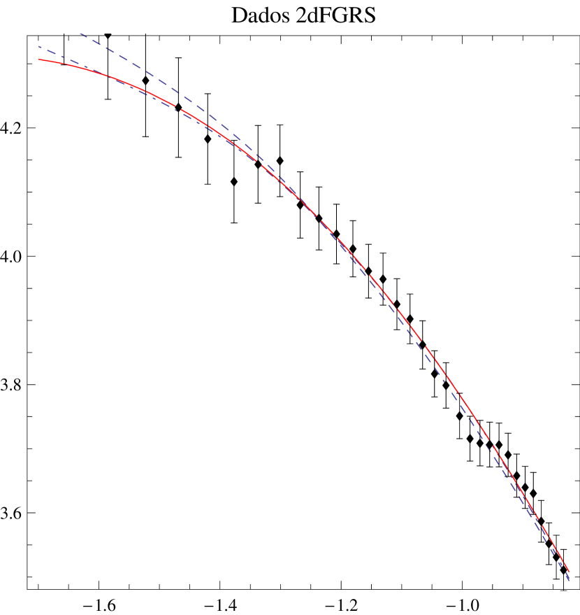
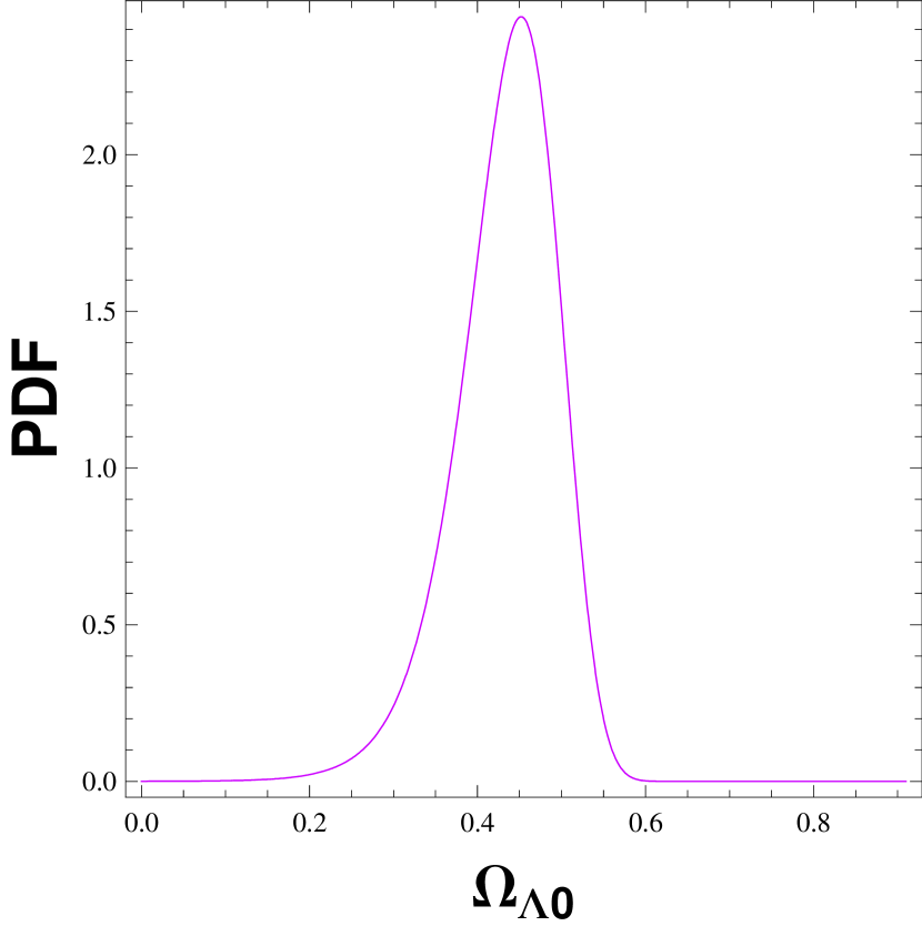
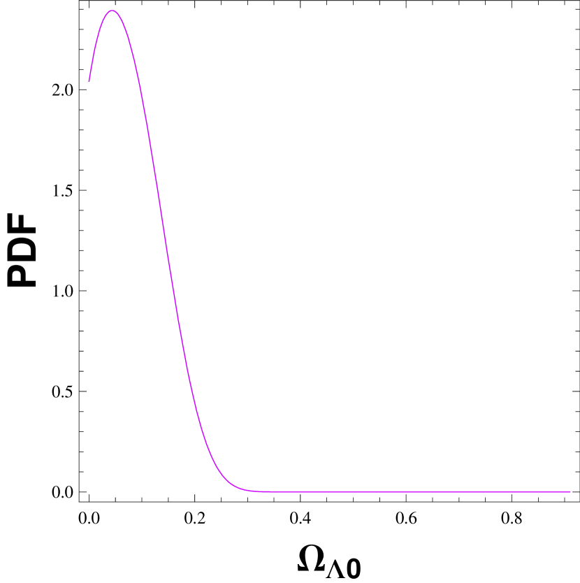
Figure 1: The best fit models for the $\Lambda$CDM model with $\Omega_{dm0}=0.24$ (continuous line), the decaying $\Lambda$ model without the perturbation of the $\Lambda$ term (dashed line) and with the perturbation in the $\Lambda$ term (dot-dashed line), when conserved baryons are not included. At the center, it is shown the PDF distribution of the dark energy density parameter when the cosmological term is not perturbed and at right the same for the case the cosmological term is perturbed.

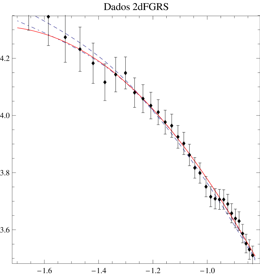
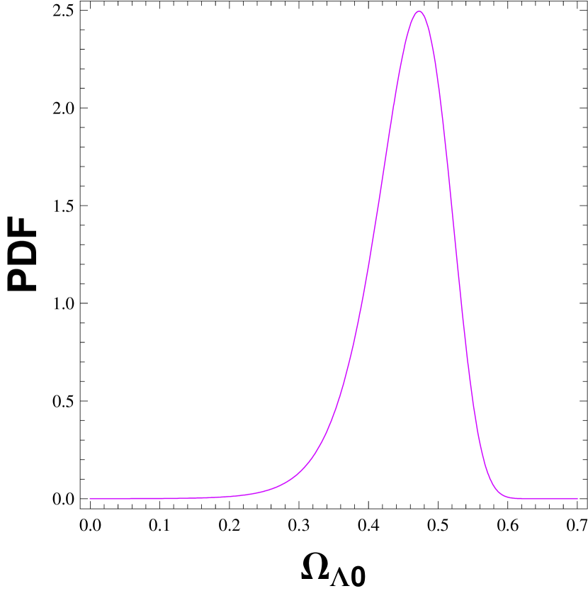
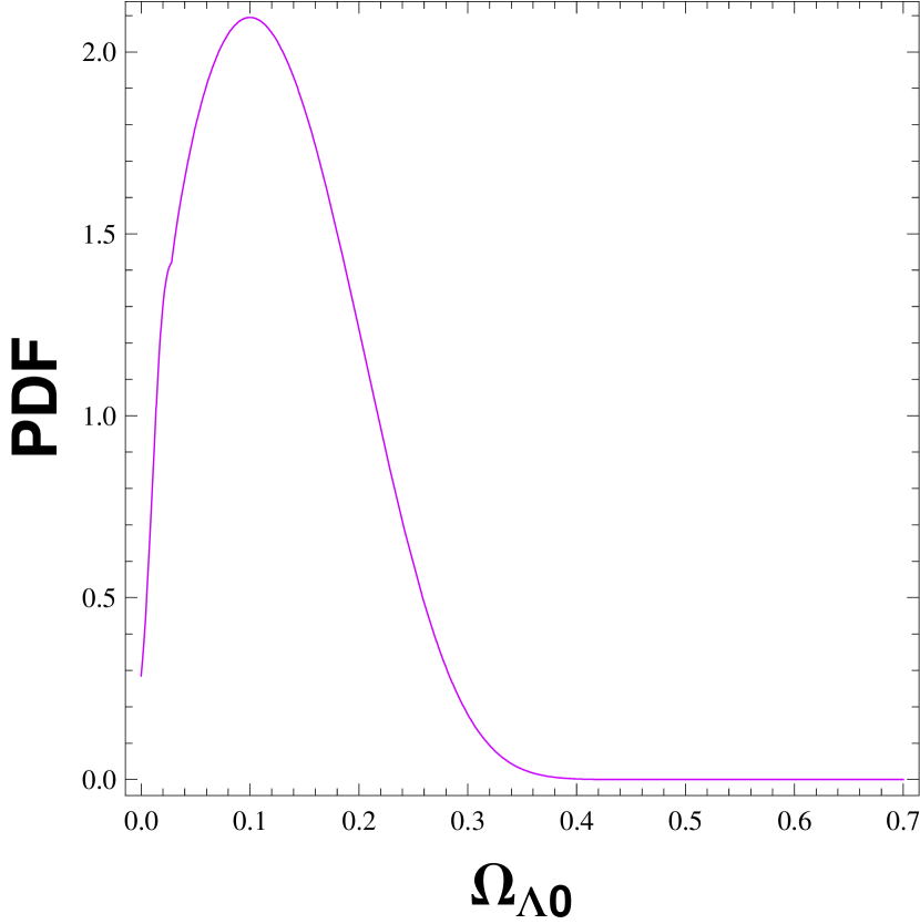
Figure 2: The best fit models for the $\Lambda$CDM model with $\Omega_{dm0}=0.24$ (continuous line), the decaying $\Lambda$ model without the perturbation of the $\Lambda$ term (dashed line) and with the perturbation in the $\Lambda$ term (dot-dashed line), when conserved baryons are included. At the center, it is shown the PDF distribution of the dark energy density parameter when the cosmological term is not perturbed and at right the same for the case the cosmological term is perturbed.

Restricting ourselves to the linear regime, we can use confidently the $\chi^{2}$ statistics, defining the statistic fitness parameter

$$\chi^{2}=\sum_{i}\biggr{(}\frac{{\cal P}_{i}^{o}-{\cal P}_{i}^{t}}{\sigma_{i}}\biggl{)}^{2},$$ (32)

where ${\cal P}_{i}^{o}$ is the observational data for the $i\,th$ value of $k$, $\sigma_{i}$ its observational error bar and ${\cal P}_{i}^{t}$ the corresponding theoretical value. This parameter depends on the densities, and from it a probability distribution can be constructed, by defining

$$F=A\exp(-\chi^{2}/2),$$ (33)

$A$ being a normalization constant.

Four situations are considered here, combining the inclusion or not of a baryonic component which is conserved separately, and the possibility that the cosmological term is perturbed or not. In Figure $1$ we exploit the case where conserved baryons are not included, which means to do $\Omega_{b0}=0$ in our system of perturbed equations. The best fitting for the $\Lambda$CDM model (with $\Omega_{dm0}=0.24$ cole ), for the case the cosmological term is not perturbed (see I ) and for the case it is perturbed are shown, together with the corresponding probability distribution function (PDF) from the $\chi^{2}$ analysis, both with a perturbation in the cosmological term and without it. The same graphics are displayed in Figure $2$, but considering the inclusion of conserved baryons, with $\Omega_{b0}=0.044$. It is easy to verify that the inclusion of the perturbation of the cosmological term displaces strongly the PDF for dark energy to the left: less dark energy is necessary, and consequently more dark matter. As an example, when conserved baryons are included, the best fitting models ask for $\Omega_{\Lambda 0}=0.47$ ($\Omega_{dm0}=0.49$) when the cosmological term is not perturbed, and $\Omega_{\Lambda 0}=0.10$ ($\Omega_{dm0}=0.86$) when $\Lambda$ is perturbed. The best fits are also shown in the table below.

	$\delta\Lambda\neq 0$, $\Omega_{b0}=0$	$\delta\Lambda=0$, $\Omega_{b0}=0$	$\delta\Lambda\neq 0$, $\Omega_{b0}=0.04$	$\delta\Lambda=0$, $\Omega_{b0}=0.04$
$\chi^{2}_{r}$	$0.31$	$0.35$	$0.31$	$0.35$
$\Omega_{dm0}$	$0.96$	$0.55$	$0.86$	$0.49$
$\Omega_{\Lambda 0}$	$0.04$	$0.45$	$0.10$	$0.47$

We can now compare our results with the other models of varying $\Lambda$ described in section II. In reference Fabris a full comparison of the theoretical results with the 2dFGRS data has been made, considering perturbations also in the cosmological term. In this model there is a free parameter represented by the constant $\sigma$. It was found that there is a very good agreement of the theoretical results with the observational data if $|\sigma|\leq 10^{-4}$. This implies that the mass of the quantum field must not be large compared with the Planck’s mass. Hence, the resulting scenario is very similar to the $\Lambda CDM$ model, which is re-obtained when $\sigma\rightarrow 0$ (no running of the cosmological constant). These results are in agreement with those of reference pavon , where a dark matter/dark energy interacting model has been studied using also matter power spectrum data: the agreement between theory and observation is assured when the interaction is very weak, that is, $\Lambda$ is a slow-varying function of time. The present model, on the other hand, does not have any free parameter that could connect it, in some limit, to the $\Lambda CDM$ model.

In reference Grande the $\Lambda XCDM$ model has been studied using also the growth of linear perturbations, and restrictions on the parameter space of the model were obtained. But the cosmological term was considered as smooth: the authors argue that the influence of the perturbations in $\Lambda$ is not significative for modes well inside the Hubble horizon, those concerned by the 2dFGRS data. A full comparison with the matter power spectra data for the $\Lambda XCDM$ model has been performed in solabis . There are two free parameters in the model, the parameter $\sigma$ which has the same meaning as in the running cosmological model of reference Fabris , and the equation of state parameter $\omega_{X}$ of the cosmon component, which exchange energy with the cosmological term. For a given region of this bidimensional parameter space the agreement with the data is excellent. Again, this happens near the cosmological constant case, which is a particular limit of those parameters.

The model of reference Holografia also implies, as we have seen, a variation of $\Lambda$ proportional to $H^{2}$. The nature of the infrared cut-off (Hubble radius, particle horizon or future event horizon) changes the effective equation of state, but not the quadratic dependence of $\rho_{\Lambda}$ on $H$. Hence, we can expect that the results using the matter power spectrum constraints should be similar to those found in reference Fabris . In their work, the authors of reference Holografia have used a Newtonian approach, imposing that the cosmological term remains a smooth component, not being perturbed. Their main results indicate that there are growing modes only when the effective equation of state implies that the energy conditions are not violated. An investigation similar to that made in the present work or in reference Fabris , considering a full relativistic approach, perturbing also the cosmological term and using extensively the 2dFGRS data, may be relevant for the case of reference Holografia .

In all these cases, we can remark that the models for which $\Lambda$ varies with $H^{2}$ contain at least one free parameter assuring that the $\Lambda CDM$ limit is contained in the model. This is not our case. Moreover, since $H$ is a small number, in the former models the variation of the cosmological term is small. A linear dependence, as we have assumed, containing no $\Lambda CDM$ limit, implies comparatively a high interaction, which seems to be ruled out by observations, in agreement with the results of reference pavon .

IV Conclusions

From a theoretical point of view, the hypothesis of vacuum decay is interesting in several aspects. First of all, it may naturally conciliate the observed cosmological term with a huge initial value for the vacuum density through a relaxing mechanism in the expanding space-time. Secondly, in the realm of our thermodynamic ansatz, we have a non-singular and inflationary early phase in the universe evolution, with the presently observed matter content generated by a primordial vacuum transition SC2 .

A late-time vacuum decay depends on the mass of the produced particles. This possibility would be interesting as an explanation for the cosmic coincidence, since the suppression of the matter contrast owing to matter production begins to have importance when the cosmological term starts to dominate the cosmic expansion I . Until now it has also been survived to a precise joint analysis of supernovas, BAO and CMB observations, with a good concordance for the two free model parameters, i.e., the present values of the Hubble constant and of the relative matter density Jailson2 .

In this paper we have extended a previous study of structure formation in this context I , investigating the consequences of matter production for the mass power spectrum. We had already shown that, in the case of a strictly homogeneous cosmological term, the suppression in the matter contrast leads to a disagreement with the observed spectrum, unless the matter density parameter is as high as $\Omega_{m0}=0.48$ (for which the accordance is excellent). This value is outside the current dynamical limits on $\Omega_{m0}$ and above the concordance value obtained from the joint analysis of supernovas, BAO and CMB, $\Omega_{m0}=0.36$ Jailson2 .

Now we have considered the possibility of perturbations in the cosmological term, a more natural assumption. Assuming that such a term presents the same scale-invariant primordial spectrum as dark matter, we conclude that the agreement with the observed spectrum, for any acceptable value of $\Omega_{m0}$, is even worse. We have also considered the case in which the initial vacuum perturbations are zero, but the fitting with observations is still bad, unless for a very high matter density. This seems to rule out a late-time running of the vacuum term, at least in the recipe of the present model.

Of course, one could test other possible amplitudes and forms for the vacuum primordial spectrum (despite its unnaturalness). In fact, we have tested a large range of amplitudes, but the obtained power spectrums are not significantly better. We have also tested values for the present mass density of decoupled particles above the baryonic mass density, supposing the presence of a massive dark particle aside the light one produced by the vacuum decay. Also in this case the fitting between the observed and predicted power spectrums is poor.

Let us remind, however, that discarding a late-time variation of the cosmological term in the present model does not mean to discard the general idea of vacuum decay. If dark energy is a manifestation of quantum vacuum in the curved, expanding background, the inclusion of a decaying cosmological term in Einstein equations is as natural as the inclusion of a genuine cosmological constant. In the realm of the present model, the disagreement with large structure observations indicates that the cosmological term does not vary at late times. Nevertheless, a different ansatz for the vacuum variation may lead to a better accordance.

Even if the vacuum decay is restricted to very early times - due to the masses of the produced particles - we have interesting consequences, as already discussed. A precise comparison of such a scenario with observations, in the context of our thermodynamic ansatz SC2 , is still in order. Particularly, its necessary to find the primordial spectrum of matter perturbations generated in the inflationary phase of the model, to be tested against the observed spectrum of anisotropies in the CMB. This research is already in progress.

References

- (1) V. Sahni and A. A. Starobinsky, Int. J. Mod. Phys. D 9, 373 (2000); T. Padmanabhan, Phys. Rept. 380, 235 (2003); P. J. E. Peebles and B. Ratra, Rev. Mod. Phys. 75, 559 (2003).
- (2) M. Ozer and O. Taha, Phys. Lett. B 171, 363 (1986); Nucl. Phys. B 287, 776 (1987); O. Bertolami, Nuovo Cimento 93, 36 (1986); K. Freese et al, Nucl. Phys. B 287, 797 (1987).
- (3) I. G. Dymnikova and M. Yu. Khlopov, Mod. Phys. Lett. A 15, 2305 (2000); R. Schützhold, Phys. Rev. Lett. 89, 081302 (2002), R. Horvat, Phys. Rev. D 70, 087301 (2004); I. Shapiro, J. Solà and H. Stefancic, JCAP 0501, 012 (2005); F. Bauer, Class. Quant. Grav. 22, 3533 (2005); J. S. Alcaniz and J. A. S. Lima, Phys. Rev. D 72, 063516 (2005); R. Aldrovandi, J. P. Beltrán and J. G. Pereira, Grav. & Cosmol. 11, 277 (2005); J. D. Barrow and T. Clifton, Phys. Rev. D 73, 103520 (2006); I. L. Shapiro and J. Solà, arXiv:0808.0315 [hep-th]; J. Grande, A. Pelinson and J. Solà, arXiv:0809.3462 [astro-ph].
- (4) S. Carneiro, Int. J. Mod. Phys. D 14, 2201 (2005); A. E. Montenegro Jr. and S. Carneiro, Class. Quant. Grav. 24, 313 (2007).
- (5) J. Grande, R. Opher, A. Pelinson and J. Solà, JCAP 0712, 007 (2007).
- (6) K. Y. Kim, H. W. Lee and Y. S. Myung, arXiv:0805.3941 [gr-qc].
- (7) W. Zimdahl and D. Pavón, Gen. Rel. Grav. 35, 413 (2003); B. Wang, Y. Gong and E. Abdalla, Phys. Lett. B 624, 141 (2005); B. Wang, C. Lin and E. Abdalla, Phys. Lett. B 637, 357 (2006); B. Wang et al., Nucl. Phys. B 778, 69 (2007); C. Feng et al., JCAP 0709, 005 (2007); E. Abdalla et al., arXiv:0710.1198 [astro-ph].
- (8) S. Bhanja, S. Chakraborty and U. Debnath, Int. J. Mod. Phys. D 14, 1919 (2005); J. S. Alcaniz, Braz. J. Phys. 36, 1109 (2006); J. P. Beltrán Almeida and J. G. Pereira, Phys. Lett. B 636, 75 (2006); J. Grande, J. Solà and H. Stefancic, JCAP 0608, 011 (2006); H. S. Zhang, Q. Guo and R. G. Cai, Mod. Phys. Lett. A 21, 159 (2006); J. P. Singh and R. K. Tiwari, Int. J. Mod. Phys. D 16, 745 (2007); F. Bauer and L. Schrempp, JCAP 0804, 006 (2008); F. E. M. Costa, J. S. Alcaniz and J. M. F. Maia, Phys. Rev. D 77, 083516 (2008); S. Funkhouser, Proc. R. Soc. A 464, 1345 (2008); Y. G. Gong and X. Chen, Phys. Rev. D 77, 103511 (2008); G. W. Ma and J. Y. Ma, Mod. Phys. Lett. A 23, 971 (2008).
- (9) J. C. Fabris, I. Shapiro and J. Sola, JCAP 0702, 016 (2007).
- (10) S. Carneiro, Int. J. Mod. Phys. D 12, 1669 (2003); Int. J. Mod. Phys. D 15, 2241 (2006); J. Phys. A 40, 6841 (2007).
- (11) H. A. Borges and S. Carneiro, Gen. Rel. Grav. 37, 1385 (2005).
- (12) S. Carneiro, C. Pigozzo, H. A. Borges and J. S. Alcaniz, Phys. Rev. D 74, 023532 (2006); S. Carneiro, M. A. Dantas, C. Pigozzo and J. S. Alcaniz, Phys. Rev. D 77, 083504 (2008).
- (13) R. Opher and A. Pelinson, Phys. Rev. D 70, 063529 (2004).
- (14) H. A. Borges, S. Carneiro, J. C. Fabris and C. Pigozzo, Phys. Rev. D 77, 043513 (2008).
- (15) R. Bousso, Rev. Mod. Phys. 74, 825 (2002).
- (16) I. L. Shapiro and J. Solà, JHEP 0202, 006 (2002).
- (17) R. Bousso, arXiv:0708.4231.
- (18) P. Astier et al., Astron. Astroph. 447, 31 (2006).
- (19) A. G. Sanchez et al., MNRAS 366, 189 (2006).
- (20) R. Colistete Jr., J. C. Fabris, J. Tossa and W. Zimdahl, Phys. Rev. D 76, 103516 (2007).
- (21) J. Martin, A. Riazuelo and M. Sakellariadou, Phys. Rev. D 61, 083518 (2000); J. M. Bardeen, J. R. Bond, N. Kaiser and A. S. Szalay, Astrophys. J. 304, 15 (1986).
- (22) S. Cole et al., MNRAS 362, 505 (2005).
- (23) M. Tegmark et al., Astrophys. J. 606, 702 (2004).
- (24) S. Cole, A.G. Sanchez and S. Wilkins, The galaxy power spectrum: 2dFRS and SDSS tension?, astro-ph/0611178.
- (25) W. J. Percival et al., MNRAS 327, 1297 (2001).
- (26) G. Olivares, F. Atrio-Barandela and D. Pavón, Phys. Rev. D74, 043521 (2006).
- (27) J. Grande, A. Pelinson and J. Solà, arXiv:0809.3462.