Fidelity susceptibility for SU(2)-invariant states

Abstract

We study the fidelity susceptibility of two SU(2)-invariant reduced density matrices. Due to the commuting property of these matrices, analytical results for reduced fidelity susceptibility are obtained and can be applied to study quantum phase transitions in SU(2)-invariant systems. As an example, we analyze the quantum criticality of the spin-one bilinear-biquadratic model via the fidelity approach.

Introduction—In 1984, Peres introduced the concept of fidelity to characterize quantum system responses to a perturbation Peres . It is of fundamental importance when studying quantum dynamics and has been applied to characterize two important phenomena in condensed matter theory, quantum chaos and quantum phase transitions (QPTs) Lloyd ; Suncp ; Zanardi ; fidelity-sspt ; HQZhou0701 ; MFYang07 ; LGong115114 . It also becomes an useful concept in quantum information theory Nielsen1 , and has been used in study of quantum entanglement theory Wei , quantum teleportation Hofmann , and transformation of unknown states Lars etc.

As an indicator of QPTs, various kinds of fidelity has been used in investigating quantum phase transition point, such as Loschmidt echo Suncp , ground-state fidelity GS-fidelity , the fidelity of first excited state FES-fidelity , operator fidelity operator-fidelity-sspt ; op , and reduced fidelity reduced-fidelity ; partial-fidelity etc. The fidelity susceptibility (FS) fidelity-sspt , as the leading term of the fidelity, can be conveniently used to detect QPTs for its independence of the concrete values of small perturbations.

Let us briefly introduce quantum fidelity and fidelity susceptibility. For pure states, fidelity is the absolute value of an overlap of two wave functions. One important case is the fidelity between the ground state $|\psi_{0}(x)\rangle$ of Hamiltonian $H(x)$ and a slightly different one $|\psi_{0}(x+\delta)\rangle$,

$$F=|\langle\psi_{0}(x)|\psi_{0}(x+\delta)\rangle|,$$ (1)

where $\delta$ is a small deviation. Substituting the expansion

$$|\psi(x+\delta)\rangle=|\psi(x)\rangle+\delta|\dot{\psi}(x)\rangle+\delta^{2}/2|\ddot{\psi}(x)\rangle+O(\delta^{3})$$ (2)

into the above equation leads to

$$F =1+\frac{\delta^{2}}{4}(\langle\psi_{0}|\ddot{\psi}_{0}\rangle+\langle\ddot{\psi}_{0}|{\psi}_{0}\rangle+2|\langle\psi_{0}|\dot{\psi}_{0}\rangle|^{2})$$

$$=1-\frac{\delta^{2}}{2}(\langle\dot{\psi}_{0}|\dot{\psi}_{0}\rangle-|\langle\psi_{0}|\dot{\psi}_{0}\rangle|^{2}).$$ (3)

One may further define the FS as fidelity-sspt

$$\chi_{F} =\lim_{\delta\rightarrow 0}\frac{2(1-F)}{\delta^{2}}=\langle\dot{\psi}_{0}|\dot{\psi}_{0}\rangle-|\langle\psi_{0}|\dot{\psi}_{0}\rangle|^{2}$$

$$=\sum_{n\neq 0}|\langle\psi_{n}|\dot{\psi}_{0}\rangle|^{2}.$$ (4)

So, the FS is explicitly written out in terms of eigenstates. However, for mixed-state case, the corresponding fidelity and FS is relatively difficult to be achieved. One can use Uhlmann’s fidelity Uhlmann

$$F=\text{tr}\sqrt{\varrho^{1/2}\widetilde{\varrho}\varrho^{1/2}}$$ (5)

for two mixed states $\varrho$ and $\widetilde{\varrho}$ and the corresponding FS can also be defined as above. In what follows, we analyze fidelity of SU(2)-invariant mixed states by this definition.

For a many-body quantum state, by tracing out other degree of freedom but two particles, we have a two-particle reduced-density matrix which is generally a mixed state. Fidelity between reduced density matrices is called reduced fidelity reduced-fidelity . For some interesting physical models such as the spin-one bilinear-biquadratic model Affleck ; Millet ; Xiang ; Botet and spin-half frustrated model, the reduced-density matrix displays a SU(2) symmetry. In this paper, we will study the fidelity of SU(2)-invariant state. The symmetry in this state faciliates greatly our study of fidelity and analytical results are obtained for the fidelity susceptibility. We also give an application of the results to study quantum phase transition in the bilinear-biquadratic model.

SU(2)-invariant states and FS— Before proceeding, we make it clear that if a multi-spin state $\rho$ displays a global SU(2) symmetry ($[\rho,\mathbf{J}]=0$), the two-spin reduced-density matrix also has a SU(2) symmetry ($[\rho_{12},\mathbf{j}_{1}+\mathbf{j}_{2}]=0$), where $\mathbf{J}=\mathbf{j}_{1}+...+\mathbf{j}_{N}$ is the collecting spin operator. The proof is straightforward. The commutator $[\rho,\mathbf{J}]=0$ means that

$$[\rho,\mathbf{j}_{1}+\mathbf{j}_{2}]=[\mathbf{j}_{3}+...+\mathbf{j}_{n},\rho].$$ (6)

After tracing out degree of freedom of spins $3\rightarrow N$, we have

$$[\rho_{12},\mathbf{j}_{1}+\mathbf{j}_{2}]=\text{Tr}_{3\rightarrow N}[\mathbf{j}_{3}+...+\mathbf{j}_{n},\rho]=0.$$ (7)

An SU(2)-invariant state of two spins $j_{1}$ and $j_{2}$ can be written in the general form

$$\rho=\sum_{J=|j_{1}-j_{2}|}^{j_{1}+j_{2}}\frac{\alpha_{J}}{2J+1}P_{J},$$ (8)

where $\alpha_{J}\geq 0$, $\sum_{J}\alpha_{J}=1$, and $P_{J}$ is the projector of spin-$J$ subspace. Obviously, the density operator has eigenvalues $\alpha_{J}/(2J+1)$ with degeneracy $2J+1$.

One key observation from the above equation is that two different SU(2)-invairant density matrices $\rho$ and $\tilde{\rho}$ commute with each other. Thus, they can be diagonalized simutaneously, and the fidelity between them are given by.

$$F=\sum_{k=1}^{j_{1}j_{2}}\sqrt{\lambda_{k}\widetilde{\lambda}_{k}},$$ (9)

where $\lambda_{k}$’s and $\widetilde{\lambda}_{k}$’s are the eigenvalues of $\rho$ and $\widetilde{\varrho}$, respectively. Since zero eigenvalues have no contribution to $F$, we only need to consider the nonzero ones. In the following, the subscript $k$ in $\sum_{k}$ only denotes nonzero eigenvalues of $\rho$.

Now we calculate fidelity of two slightly different density matrices $\rho(x)$ and $\rho(x+\delta)$ as a function of parameter $x$, where $\delta$ is a small change of $x$. It is noticed that, for a small change $\delta,$ we have

$${\lambda_{k}(x+\delta)}\simeq\lambda_{k}+\left(\partial_{x}\lambda_{k}\right)\delta+\left(\partial_{x}^{2}\lambda_{k}\right)\delta^{2}/{2}+O\left(\delta^{3}\right).$$ (10)

Substituting this expression into Eq. (9) leads to the fidelity given by

$$F=1-\frac{\delta^{2}}{2}\sum_{i}\frac{\left(\partial_{x}\lambda_{k}\right)^{2}}{4\lambda_{k}}.$$ (11)

In deriving the above equation, we have used $\sum_{i}\lambda_{i}\equiv{1}$ and $\sum_{i}\partial_{\alpha}\lambda_{i}=\sum_{i}\partial_{\alpha}^{2}\lambda_{i}=0.$ Therefore, according to the relation between fidelity and FS $F=1-\chi{\delta^{2}/2}$ fidelity-sspt , the FS $\chi_{F}$ corresponding to the matrix $\rho$ is obtained as

$$\chi_{F}=\sum_{k}\frac{\left(\partial_{x}\lambda_{k}\right)^{2}}{4\lambda_{k}}.$$ (12)

This expression of fidelity susceptibility is valid for any commuting density matrices. It depends on nonzero eigenvalues of $\rho$ and their first-order derivatives.

Applying the Eq. (12) to the SU(2)-invariant state $\rho$ (8), one obtains the FS for $\rho$ as

$$\chi_{F}=\sum_{J=j_{2}-j_{1}}^{j_{1}+j_{2}}\frac{(\partial_{x}\alpha_{J})^{2}}{4\alpha_{J}},$$ (13)

where we assumed $j_{2}>j_{1}$ without loss of generality. Now, we consider the following case of $j_{1}=1/2$ and $j_{2}\geq 1/2$. As $\alpha_{j_{2}-1/2}+\alpha_{j_{2}+1/2}=1$, Eq. (13) reduces to

$$\chi_{F}=\frac{(\partial_{x}\alpha_{j_{2}-1/2})^{2}}{4\alpha_{j_{2}-1/2}(1-\alpha_{j_{2}-1/2})}.$$ (14)

Parameter $\alpha_{j_{2}-1/2}$ can be written in terms of expectation of Heisenberg interaction on $\rho$, $\langle\mathbf{j}_{1}\cdot\mathbf{j}_{2}\rangle$, i.e.,  Schliemann

$$\alpha_{j_{2}-1/2}=\frac{1}{2j_{2}+1}(j_{2}-2\langle\mathbf{j}_{1}\cdot\mathbf{j}_{2}\rangle).$$ (15)

Thus, Eq. (14) can be reexpressed in the following form

$$\chi_{F}=\frac{(\partial_{x}\langle\mathbf{j}_{1}\cdot\mathbf{j}_{2}\rangle)^{2}}{(j_{2}-2\langle\mathbf{j}_{1}\cdot\mathbf{j}_{2}\rangle)(j_{2}+1+2\langle\mathbf{j}_{1}\cdot\mathbf{j}_{2}\rangle)}$$ (16)

We see that for the SU(2)-invariant state, the FS is completely determined by the expectation value of Heisenberg interaction and its first-order derivative. If we consider the case of two qubits, then the above equation reduces to

$$\chi_{F}=\frac{4(\partial_{x}\langle\mathbf{j}_{1}\cdot\mathbf{j}_{2}\rangle)^{2}}{(1-4\langle\mathbf{j}_{1}\cdot\mathbf{j}_{2}\rangle)(3+4\langle\mathbf{j}_{1}\cdot\mathbf{j}_{2}\rangle)},$$ (17)

which is just the FS obtained in Ref. Xiong via a different approach.

Now, we study the case of two qutrits, i.e., two spin ones. From Eq. (8), one has

$$\alpha_{0} =\langle P_{0}\rangle=\langle P_{12}\rangle,$$

$$\alpha_{1} =\langle P_{1}\rangle=\frac{1}{2}(1-\langle S_{12}\rangle),$$

$$\alpha_{2} =\langle P_{2}\rangle=\frac{1}{2}(1-2\langle P_{12}\rangle+\langle S_{12}\rangle),$$ (18)

where

$$P_{12} =\frac{1}{3}[(\mathbf{j}_{1}\cdot\mathbf{j}_{2})^{2}-1],$$

$$S_{12} =\mathbf{j}_{1}\cdot\mathbf{j}_{2}+(\mathbf{j}_{1}\cdot\mathbf{j}_{2})^{2}-1,$$ (19)

are singlet projection operator and swap operator, respectively. Substituting Eqs. (Fidelity susceptibility for SU(2)-invariant states) and (Fidelity susceptibility for SU(2)-invariant states) into Eq. (13) leads to the FS for two qutrits

$$\chi_{F} =\frac{1}{4}\left[{\Huge\frac{(\partial_{x}\langle P_{12}\rangle)^{2}}{\langle P_{12}\rangle}+\frac{(\partial_{x}\langle S_{12}\rangle)^{2}}{2(1-\langle S_{12}\rangle)}}\right.$$

$$\left.+\frac{(\partial_{x}\langle S_{12}\rangle-2\partial_{x}\langle P_{12}\rangle)^{2}}{2(1-2\langle P_{12}\rangle+\langle S_{12}\rangle)}\right]{\huge,}$$ (20)

The FS is detrmined by two expectation values $\langle P_{12}\rangle$ and $\langle S_{12}\rangle$ and their first-order derivatives. Below, we will apply this formula to the study of the bilinear-biquadratic model.

Applications to spin-one systems— Spin Heisenberg chains attract more attention since Haldane predicted that the one-dimensional chain has a spin gap for integer spins Haldane . In these studies, the bilinear-biquadratic model has played an important role Affleck ; Millet ; Xiang ; Botet . The corresponding Hamiltonian is given by

$$H_{BB} = \sum_{i=1}^{N}\cos\theta\left(\mathbf{j}_{i}\cdot\mathbf{j}_{i+1}\right)+\sin\theta\left(\mathbf{j}_{i}\cdot\mathbf{j}_{i+1}\right)^{2},$$

$$= \sum_{i=1}^{N}[\cos\theta S_{i,i+1}+3(\sin\theta-\cos\theta)P_{i,i+1}]+N\sin\theta.$$

In deriving the last equality, we have used Eq. (Fidelity susceptibility for SU(2)-invariant states). Here, $\mathbf{j}_{i}$ denotes spin-1 operator at site $i$, and we have assumed the periodic boundary conditions. The Hamiltonian exhibits a SU(2) symmetry, and displays very rich quantum phase diagrams Schollwock .

From Hellmann-Feymann theorem for ground state, one can easily find that

$$\langle P_{12}\rangle =\frac{1}{3}(\sin\theta e_{0}+\cos\theta e_{0}^{\prime}-1),$$

$$\langle S_{12}\rangle =(\cos\theta+\sin\theta)e_{0}+(\cos\theta-\sin\theta)e_{0}^{\prime}-1,$$ (22)

and the their first-order derivatives

$$\langle P_{12}\rangle^{\prime} =\frac{\cos\theta}{3}(e_{0}+e_{0}^{\prime\prime}),$$

$$\langle S_{12}\rangle^{\prime} =({\cos\theta-\sin\theta})(e_{0}+e_{0}^{\prime\prime}),$$

$$\langle S_{12}\rangle^{\prime}-2\langle P_{12}\rangle^{\prime} =\left(\frac{\cos\theta}{3}-\sin\theta\right)(e_{0}+e_{0}^{\prime\prime}).$$ (23)

Here, $e_{0}$ denotes the ground-state energy per site. Substituting the above two equations into (Fidelity susceptibility for SU(2)-invariant states), one obtains the FS in terms of $e_{0}$, $e_{0}^{\prime}$, and $e_{0}^{\prime\prime}$ as follows

$$\chi_{F} =\frac{(e_{0}+e_{0}^{\prime\prime})^{2}}{4}\left[\frac{\cos^{2}\theta}{3(\sin\theta e_{0}+\cos\theta e_{0}^{\prime}-1)}\right.$$

$$+\frac{(\cos\theta-\sin\theta)^{2}}{2[2-(\cos\theta+\sin\theta)e_{0}-(\cos\theta-\sin\theta)e_{0}^{\prime}]}$$

$$\left.+\frac{(\cos\theta-3\sin\theta)^{2}}{6[2+(3\cos\theta+\sin\theta)e_{0}+(\cos\theta-3\sin\theta)e_{0}^{\prime}]}\right]$$ (24)

One key observation is that the numerators of the above two expressions happen to be proportional to $(e_{0}+e_{0}^{\prime\prime})^{2}$. Then, we infer that if the second derivative of the ground-state energy is singular at the critical point, the FS is singular too. On the other hand, it is known that the divergence of the second derivative of the ground-state energy reflects the second-order QPTs of the system, which is shown in Ref. GS-fidelity explicitly as

$$\partial_{\alpha}^{2}e_{0}=\sum_{n\neq 0}^{N}\frac{2\left|\langle\Psi_{n}|\partial_{\alpha}H|\Psi_{n}\rangle\right|^{2}}{N(E_{0}-E_{n})},$$

where $|\Psi_{n}\rangle$ is the eigenvector corresponding to the eigenvalue $E_{n}$. It shows that the vanishing energy gap in the thermodynamic limit can lead to the singularity of the the second derivative of the ground-state energy. Therefore, the two-spin FSs can exactly reflects the second-order QPTs of the global system in this model.

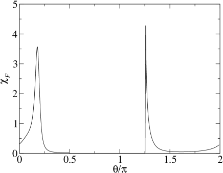
Figure 1: Ground-state fidelity susceptibility as a function of $\theta/\pi$ in the bilinear-biquadratic model.

We use the exact-diagonalization method to calcuate the ground-state energy and then numerical results of FS is obtained from Eq.(Fidelity susceptibility for SU(2)-invariant states) . In Fig. 1, we plot the FS as a function of $\theta$ for a sample of 12 spins. We observe a sharp decrease of the FS around $\theta=\pi/4$, which separate the Haldane phase ($-\pi/4<\theta<\pi/4$) and the trimerized phase ($\pi/4<\theta<\pi/2$). This may imply that a QPT occurs. For $\pi/2<\theta<5\pi/4$, the ground state is ferromagnetic and degenerate. In this range, the FS is zero. However, at $\theta=7\pi/4$, corresponding to a QPT point separating dimerized phase ($5\pi/4<\theta<7\pi/4$) and Haldane phase, one cannot find any anomalous behaviors of the FS.

Conclusions—We have studied the FS in SU(2)-invariant states and have obtained exact analytical expression of the FS for any spins $j_{1}$ and $j_{2}$. This implies that the results are applicable to not only equal-spin but also mixed-spin systems. Furthermore, one can use the FS to study properties of SU(2)-invariant physical systems in a finite-temperature thermal state. As an application, we have studied relations between the FS and QPTs in the bilinear-biquadratic model. For this model, one can infer that the two-spin FS can exactly reflects the second-order QPTs of the global system. Here, we restrict us to study SU(2)-invariant states of two spins, after tracing out other spins of a many-body states. One challenge for further investigation is to study $N$-spin ($N\geq 3$) SU(2)-invariant reduced density matrix.

Acknowledgements This work was supported by the Program for New Century Excellent Talents in University (NCET), the NSFC with grant No. 90503003, the State Key Program for Basic Research of China with grant No. 2006CB921206, the Specialized Research Fund for the Doctoral Program of Higher Education with grant No. 20050335087, and the Direct grant of CUHK (A/C 2060344). X. Wang acknowledge the support from C. N. Yang fellowship via CUHK.

References

- (1) A. Peres, Phys. Rev. A 30, 1610 (1984).
- (2) Y. Weinstein, S. Lloyd, and C. Tsallis, Phys. Rev. Lett. 89, 214101 (2002).
- (3) H. T. Quan, Z. Song, X. F. Liu, P. Zanardi, and C. P. Sun, Phys. Rev. Lett. 96, 140604 (2006).
- (4) P. Zanardi and N. Paunković, Phys. Rev. E 74, 031123 (2006).
- (5) W. L. You, Y. W. Li, and S. J. Gu, Phys. Rev. E 76, 022101 (2007).
- (6) H. Q. Zhou and J. P. Barjaktarevic, arXiv: cond-mat/0701608.
- (7) M. F. Yang, Phys. Rev. B 76, 180403 (R) (2007).
- (8) L. Gong and P. Tong, Phys. Rev. B 78, 115114 (2008).
- (9) M. A. Nilesen and I. L. Chuang, Quantum Computation and Quantum Information (Cambridge University Press, Cambridge, England, 2000).
- (10) T. C Wei and P. M. Goldbart, Phys. Rev. A 68, 042307 (2003).
- (11) H. F. Hofmann, T. Ide, T. Kobayashi, and A. Furusawa, Phys. Rev. A 62, 062304 (2000).
- (12) L. B. Madsen and K. Mølmer, Phys. Rev. A 73, 032342 (2006).
- (13) S. Chen, L. Wang, Y. Hao, and Y. Wang, Phys. Rev. A 77, 032111 (2008).
- (14) S. Chen, L. Wang, S. J. Gu, and Y. Wang, Phys. Rev. E 76, 061108 (2007).
- (15) X. Wang, Z. Sun, and Z. D. Wang, arXiv:0803.2940.
- (16) X. M. Lu, Z. Sun, X. Wang, P. Zanardi, Phys. Rev. A78, 032309 (2008).
- (17) J. Ma, L. Xu, H. Xiong, and X. Wang, arXiv:0805.4062.
- (18) N. Paunković, P. D. Sacramento, P. Nogueira, V. R. Vieira, and V. K. Dugaev, Phys. Rev. A 77, 052302 (2008); H. M. Kwok, C. S. Ho and S. J. Gu, arXiv:0805.3885.
- (19) D. Bures, Tran. Am. Math. Soc. 135, 199 (1969); A. Uhlmann, Rep. Math. Phys. 9 273 (1976); R. Jozsa, J. Mod. Opt. 41 2315 (1994).
- (20) I. Affleck, T. Kennedy, E. H. Lieb, and H. Tasaki, Phys. Rev. Lett. 59, 799 (1987).
- (21) P. Millet, F. Mila, F. C. Zhang, M. Mambrini, A. B. Van Oosten, V. A. Pashchenko, A. Sulpice, and A. Stepanov, Phys. Rev. Lett. 83, 4176 (1999).
- (22) J. Z. Lou, T. Xiang, and Z. B. Su, Phys. Rev. Lett. 85, 2380 (2000).
- (23) R. Botet and R. Jullien, Phys. Rev. B 27, 613 (1983).
- (24) J. Schliemann, Phys. Rev. A68, 012309 (2003).
- (25) H. N. Xiong, J. Ma, Z. Sun, and X. Wang, arXiv:0808.1817
- (26) F. D. M. Haldane, Phys. Lett. 93A, 464 (1983); F. D. M. Haldane, Phys. Rev. Lett. 50, 1153 (1983).
- (27) U. Schollwöck, T. Jolicoeur, and T. Garel, Phys. Rev. B53, 3304 (1996).