Noise induced Hopf bifurcation

Abstract

We consider effect of stochastic sources upon self-organization process being initiated with creation of the limit cycle induced by the Hopf bifurcation. General relations obtained are applied to the stochastic Lorenz system to show that departure from equilibrium steady state can destroy the limit cycle in dependence of relation between characteristic scales of temporal variation of principle variables. Noise induced resonance related to the limit cycle is found to appear if the fastest variations displays a principle variable, which is coupled with two different degrees of freedom or more.

I Introduction

Interplay between noise and non-linearity of dynamical systems 1 is known to arrive at crucial changing in behavior of systems displaying noise-induced 2 ; 2a and recurrence 3a ; 3 phase transitions, stochastic resonance 4a ; 4 , noise induced pattern formation a ; b , and noise induced transport c ; 2a . The constructive role of noise on dynamical systems includes hopping between multiple stable attractors e ; f , stabilization of the Lorenz attractor near the threshold of its formation d ; g and stabilization of resonance related to the limit cycle near the Hopf bifurcation d . Such type behavior is inherent in systems which involve discrete entities (for instance, in ecological systems individuals form population stochastically in accordance with random births and deaths). Examples of substantial alteration of finite systems under effect of intrinsic noises gives epidemics 11 –13 , predator-prey population dynamics 5 ; 6 , opinion dynamics 10 , biochemical clocks 15 ; 16 , genetic networks 14 , cyclic trapping reactions 9 , etc. Within the phase-plane language, phase transitions pointed out present the simplest case, where a fixed point appears only. We are interested in studying more complicated situation, when the system under consideration may display oscillatory behavior related to the limit cycle appearing as result of the Hopf bifurcation 17 ; 18 . It has long been conjectured 19 that in some situations the influence of noise would be sufficient to produce cyclic behavior 20 . Recent consideration 21 allows the relation between the stochastic oscillations in the fixed point phase and the oscillations in the limit cycle phase to be elucidated. In the last case, making use of co-moving frame allows fluctuations transverse and longitudinal with respect to the limit cycle to be effectively decoupled. It appears while the latter fluctuations are of a diffusive nature, the former ones follow a stochastic path. To formulate related model we consider the system with a finite number of constituents related to components of the state vector 22

$${\bf n}=N{\bf X}+\sqrt{N}{\bf x}.$$ (1)

Characteristically, a deterministic component $\bf X$ is proportional to total system size $N<\infty$, whereas a random one ${\bf x}$ is the same to its square root. In the limit of infinite particle numbers $N\to\infty$, such systems are faithfully described by deterministic equations to find time dependence ${\bf X}(t)$, which addresses the behavior of the system on a mean-field level. On the other hand, a systematic study of corrections due to finite system size can capture the behavior of fluctuations ${\bf x}(t)$ about the mean-field solution. These fluctuations are governed with the Langevin equations, however, in difference of approach 21 , we consider multiplicative noises instead of additive ones, on the one hand, and nonlinear forces instead of linear ones, on the other. Within such framework, the aim of the present paper is to extend analytical descriptions 21 of finite-size stochastic effects to systems where noises play a crucial role with respect to periodic limit cycle solution creation or its supression. We will show that character of the system behavior is determined with relation between scales of temporal variation of principle variables and their coupling.

The paper is organized along the following lines. In Section II, we obtain conditions of the limit cycle creation making use the pair of stochastic equations with nonlinear forces and multiplicative noises. Sections III, IV are devoted to consideration of these conditions on the basis of stochastic Lorenz system with different regimes of principle variables slaving. According to Section III the limit cycle is created only in the case if the most fast variation displays a principle variable, which is coupled nonlinearly with two degrees of freedom or more. Opposite case is studied in Section IV to show that the limit cycle disappears in non equilibrium steady state. Section V concludes our consideration.

II Statistical picture of limit cycle

According to the theorem of central manifold 17 , to achieve a closed description of a limit cycle it is enough to use only two variables $x_{\alpha}$, $\alpha=1,2$. In such a case, stochastic evolution of the system under investigation is defined by the Langevin equations 23

$$\dot{x}_{\alpha}=f^{(\alpha)}+\mathcal{G}_{\alpha}\zeta(t),\quad\alpha=1,2$$ (2)

with forces $f^{(\alpha)}=f^{(\alpha)}(x_{1},x_{2})$ and noise amplitudes $\mathcal{G}_{\alpha}=\mathcal{G}_{\alpha}(x_{1},x_{2})$, being functions of stochastic variables $x_{\alpha}$, $\alpha=1,2$, and white noise $\zeta(t)$ determined as usually: $\langle\zeta(t)\rangle=0$, $\langle\zeta(t)\zeta(t^{\prime})\rangle=\delta(t-t^{\prime})$. Our principle assumptions are as follows: (i) white noise $\zeta(t)$ is equal for both degrees of freedom $x_{\alpha}$; (ii) microscopic transfer rates are non correlated for different variables $x_{\alpha}$. Then, the probability distribution function $\mathcal{P}=\mathcal{P}(x_{1},x_{2};t)$ is determined by the Fokker-Planck equation

$$\frac{\partial\mathcal{P}}{\partial t}+\frac{\partial J^{\alpha}}{\partial x_{\alpha}}=0,$$ (3)

where sum over repeated Greek indexes $\alpha=1,2$ is meant and components of the probability current take the form

$$J^{(\alpha)}\equiv\mathcal{F}^{(\alpha)}\mathcal{P}-\frac{1}{2}\frac{\partial}{\partial x_{\beta}}\left(\mathcal{G}_{\alpha}\mathcal{G}_{\beta}\mathcal{P}\right),$$ (4)

with the generalized forces

$$\mathcal{F}^{(\alpha)}=f^{(\alpha)}+\lambda\frac{\partial\left(\mathcal{G}_{\alpha}\mathcal{G}_{\beta}\right)}{\partial x_{\beta}}$$ (5)

being determined with choice of the calculus parameter $\lambda\in[0,1]$. Within the steady state, the components of the probability current take constant values $J^{(\alpha)}_{0}$ and the system behaviour is defined by the following equations:

$$\frac{\partial}{\partial x_{1}}\left(\mathcal{G}_{1}^{2}\mathcal{P}\right)+\frac{\partial}{\partial x_{2}}\left(\mathcal{G}_{1}\mathcal{G}_{2}\mathcal{P}\right)-2\mathcal{F}^{(1)}\mathcal{P}=-2J^{(1)}_{0},$$ (6)

$$\frac{\partial}{\partial x_{1}}\left(\mathcal{G}_{1}\mathcal{G}_{2}\mathcal{P}\right)+\frac{\partial}{\partial x_{2}}\left(\mathcal{G}_{2}^{2}\mathcal{P}\right)-2\mathcal{F}^{(2)}\mathcal{P}=-2J^{(2)}_{0}.$$ (7)

Multiplying the first of these equations by factor $\mathcal{G}_{2}$ and the second one by $\mathcal{G}_{1}$ and then subtracting results, we arrive at the explicit form of the probability distribution function as follows:

$$\mathcal{P}\left(x_{1},x_{2}\right)=\frac{J^{(1)}_{0}\mathcal{G}_{2}\left(x_{1},x_{2}\right)-J^{(2)}_{0}\mathcal{G}_{1}\left(x_{1},x_{2}\right)}{\mathcal{D}\left(x_{1},x_{2}\right)},$$

$$\mathcal{D}\left(x_{1},x_{2}\right)\equiv\left(\mathcal{G}_{2}\mathcal{F}^{(1)}-\mathcal{G}_{1}\mathcal{F}^{(2)}\right)$$ (8)

$$+\frac{1}{2}\left[\left(\mathcal{G}_{1}^{2}\frac{\partial\mathcal{G}_{2}}{\partial x_{1}}-\mathcal{G}_{2}^{2}\frac{\partial\mathcal{G}_{1}}{\partial x_{2}}\right)-\mathcal{G}_{1}\mathcal{G}_{2}\left(\frac{\partial\mathcal{G}_{1}}{\partial x_{1}}-\frac{\partial\mathcal{G}_{2}}{\partial x_{2}}\right)\right].$$

This function diverges at condition

$$2\left(\mathcal{G}_{1}\mathcal{F}^{(2)}-\mathcal{G}_{2}\mathcal{F}^{(1)}\right)$$

$$=\left(\mathcal{G}_{1}^{2}\frac{\partial\mathcal{G}_{2}}{\partial x_{1}}-\mathcal{G}_{2}^{2}\frac{\partial\mathcal{G}_{1}}{\partial x_{2}}\right)-\mathcal{G}_{1}\mathcal{G}_{2}\left(\frac{\partial\mathcal{G}_{1}}{\partial x_{1}}-\frac{\partial\mathcal{G}_{2}}{\partial x_{2}}\right).$$ (9)

that physically means appearance of a domain of forbidden values of stochastic variables $x_{\alpha}$, which is bonded with a closed line of the limit cycle. Characteristically, such a line appears if the denominator $\mathcal{D}(x_{1},x_{2})$ of fraction (II) includes even powers of both variables $x_{1}$ and $x_{2}$.

It is worth to note the analytical expression (II) of the probability distribution function becomes possible due to the special form of the probability current (4), where effective diffusion coefficient takes the multiplicative form $\mathcal{D}_{\alpha\beta}=\mathcal{G}_{\alpha}\mathcal{G}_{\beta}$. In general case, this coefficient is known 24 to be defined with the expression

$$\mathcal{D}_{\alpha\beta}=\sum\limits_{ab}I_{ab}g_{\alpha}^{a}g_{\beta}^{b},$$ (10)

where kernel $I_{ab}$ determines transfer rate between microscopic states $a$ and $b$, whereas factors $g_{\alpha}^{a}$ and $g_{\beta}^{b}$ are specific noise amplitudes of values $x_{\alpha}$ related to these states. We have considered above the simplest case, when the transfer rate $I_{ab}=I$ is constant for all microscopic states. As a result, the diffusion coefficient (10) takes the needed form $\mathcal{D}_{\alpha\beta}=\mathcal{G}_{\alpha}\mathcal{G}_{\beta}$ with cumulative noise amplitudes $\mathcal{G}_{\alpha}\equiv\sqrt{I}\sum_{a}g_{\alpha}^{a}$ and $\mathcal{G}_{\beta}\equiv\sqrt{I}\sum_{b}g_{\beta}^{b}$.

III Noise induced resonance within Lorenz system

As the simplest and most popular example of the self-organization induced by the Hopf bifurcation, we consider modulation regime of spontaneous laser radiation, whose behaviour is presented in terms of the radiation strength $E$, the matter polarization $P$ and the difference of level populations $S$ 22 . With accounting for stochastic sources related, the self-organization process of this system is described by the Lorenz equations

$$\tau_{E}\dot{E}=[-E+a_{E}P-\varphi(E)]+g_{E}\zeta(t),$$

$$\tau_{P}\dot{P}=(-P+a_{P}ES)+g_{P}\zeta(t),$$ (11)

$$\tau_{S}\dot{S}=[(S_{e}-S)-a_{S}EP]+g_{S}\zeta(t).$$

Here, overdot denotes differentiation over time $t$; $\tau_{E,P,S}$ and $a_{E,P,S}>0$ are time scales and feedback constants of related variables, respectively; $g_{E,P,S}$ are corresponding noise amplitudes, and $S_{e}$ is driven force. In the absence of noises $(g_{E}=g_{P}=g_{S}=0)$ and at relation $\tau_{P},\tau_{S}\ll\tau_{E}$ between time scales, the system addresses to limit cycle only in the presence of the nonlinear force 25

$$\varphi(E)=\frac{\kappa E}{1+E^{2}/E_{n}^{2}}$$ (12)

characterized with parameters $\kappa>0$ and $E_{n}$. In this Section, we consider noise effect in the case of opposite relation $\tau_{E}\ll\tau_{P},\tau_{S}$ of time scales, when periodic variation of stochastic variables becomes possible even at suppression of the force (12).

It is convenient further to pass to dimensionless variables $t$, $\zeta$, $E$, $P$, $S$, $g_{E}$, $g_{P}$, $g_{S}$ with making use of the related scales:

$$\tau_{P};\quad\zeta_{s}=\tau_{E}^{-1/2};\quad E_{s}=(a_{P}a_{S})^{-1/2},$$

$$P_{s}=(a^{2}_{E}a_{P}a_{S})^{-1/2},\quad S_{s}=(a_{E}a_{P})^{-1};$$ (13)

$$g_{E}^{s}=(\tau_{P}/a_{P}a_{S})^{1/2},\quad g_{P}^{s}=(\tau_{P}/a^{2}_{E}a_{P}a_{S})^{1/2},$$

$$g_{S}^{s}=\tau_{P}^{1/2}/a_{E}a_{P}.$$

Then, equations (III) (these equations are reduced to initial form 22a if one set there $X\equiv\sqrt{\sigma/\varepsilon}E$, $Y\equiv\sqrt{\sigma/\varepsilon}P$, $Z\equiv S_{e}-S$, $r\equiv S_{e}$, and $b\equiv\sigma/\varepsilon$.) take the simple form

$$\sigma^{-1}\dot{E}=-E+P-\varphi(E)+g_{E}\zeta(t),$$

$$\dot{P}=-P+ES+g_{P}\zeta(t),$$ (14)

$$(\varepsilon/\sigma)\dot{S}=(S_{e}-S)-EP+g_{S}\zeta(t),$$

where the time scale ratios

$$\sigma\equiv\tau_{P}/\tau_{E},\quad\varepsilon\equiv\tau_{S}/\tau_{E}$$ (15)

are introduced. In the absence of noises, the Lorenz system (III) is known to show the usual bifurcation in the point $S_{e}=1$ and the Hopf bifurcation at the driven force 22a ; 22

$$S_{e}=\frac{\tau_{P}}{\tau_{E}}~{}\frac{\tau_{E}^{-1}+\tau_{S}^{-1}+3\tau_{P}^{-1}}{\tau_{E}^{-1}-\tau_{S}^{-1}-\tau_{P}^{-1}}.$$ (16)

However, at $g_{E}=g_{P}=g_{S}=0$ the limit cycle is unstable and the Hopf bifurcation arrives at the strange attractor only.

With switching on noises, the condition $\tau_{E}\ll\tau_{P}$ allows for to put l.h.s. of the first equation (III) to be equal zero. Then, the strength is expressed with the equality

$$E=P+g_{E}\zeta(t),$$ (17)

whose insertion into the system (III) reduces it into two-dimensional form

$$\dot{P}=-P(1-S)+G_{P}\zeta(t),$$

$$\dot{S}=(\sigma/\varepsilon)\left[(S_{e}-S)-P^{2}\right]+G_{S}\zeta(t)$$ (18)

with the effective amplitudes of multiplicative noises

$$\mathcal{G}_{P}\equiv\sqrt{g_{P}^{2}+g_{E}^{2}S^{2}},\quad\mathcal{G}_{S}\equiv(\tau_{P}/\tau_{S})\sqrt{g_{S}^{2}+g_{E}^{2}P^{2}}$$ (19)

and the generalized forces

$$\mathcal{F}^{(P)}=-P(1-S)+\lambda\frac{g_{E}^{2}}{\tau_{S}/\tau_{P}}S\sqrt{\frac{(g_{S}/g_{E})^{2}+P^{2}}{(g_{P}/g_{E})^{2}+S^{2}}},$$

$$\mathcal{F}^{(S)}=(\tau_{P}/\tau_{S})\left[(S_{e}-S)-P^{2}\right]$$ (20)

$$+\lambda\frac{g_{E}^{2}}{\tau_{S}/\tau_{P}}P\sqrt{\frac{(g_{P}/g_{E})^{2}+S^{2}}{(g_{S}/g_{E})^{2}+P^{2}}}.$$

In this way, the probability density (II) takes infinite values at condition

$$\left(\frac{g_{S}^{2}}{g_{E}^{2}}+P^{2}\right)\sqrt{\frac{g_{P}^{2}}{g_{E}^{2}}+S^{2}}P(1-S)$$

$$+\left(\frac{g_{P}^{2}}{g_{E}^{2}}+S^{2}\right)\sqrt{\frac{g_{S}^{2}}{g_{E}^{2}}+P^{2}}\left[(S_{e}-S)-P^{2}\right]$$ (21)

$$+\frac{g_{E}^{2}}{2}\frac{\sigma}{\varepsilon}\left(\frac{g_{S}^{2}}{g_{E}^{2}}+P^{2}\right)^{\frac{3}{2}}S-\frac{g_{E}^{2}}{2}\left(\frac{g_{P}^{2}}{g_{E}^{2}}+S^{2}\right)^{\frac{3}{2}}P=0,$$

where we choose the simplest case of Ito calculus $(\lambda=0)$.

Reduced Lorenz system (III) has two-dimensional form (2), where the role of variables $x_{1}$ and $x_{2}$ play the matter polarization $P$ and the difference of level populations $S$. According to the distribution function (II) shown in Fig.1, the stochastic

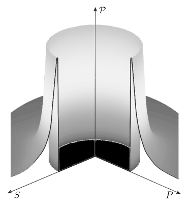
Figure 1: Steady-state distribution function (II) at $J^{(P)}_{0}=1$, $J^{(S)}_{0}=10$, $\tau_{P}=\tau_{S}$, $S_{e}=0.5$, $g_{E}=0.5$, $g_{P}=1.376$, $g_{S}=2.5$

variables $P$ and $S$ are realized with non-zero probabilities out off the limit cycle only, whereas in its interior the domain of forbidden values $P$, $S$ appears. That is principle difference from the deterministic limit cycle, which bounds a domain of unstable values of related variables. The form of this domain is shown in Fig.2

a                                 b

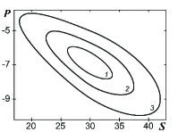
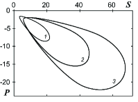
Figure 2: Form of limit cycle at: a) $g_{E}=0.5$, $g_{P}=11$, $g_{S}=6$ (curves 1-3 relate to $S_{E}=0.5,1.0,2.0$, correspondingly); b) $S_{e}=0.5$, $g_{P}=7.5$, $g_{S}=6.5$ (curves 1-3 relate to $g_{E}=1.0,0.6,0.5$, correspondingly)

at different values of the noise amplitudes $g_{E}$, $g_{P}$, $g_{S}$ and driven force $S_{e}$. It is seen, this domain grows with increase of the driven force $S_{E}$, whereas increase of the force fluctuations $g_{E}$ shrinks it. On the other hand, phase diagrams depicted in Fig.3 show

a                                 b

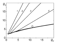
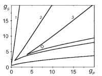
Figure 3: Phase diagrams of the limit cycle creation determined with Eq.(III) at: a) $g_{E}=0.5$, curves 1-4 correspond to $S_{e}=0.0,0.5,1.0,2.0$, respectively; b) $S_{e}=0.5$, curves 1-3 correspond to $g_{E}=0.1,0.5,1.0$, respectively (diamonds relate to the values $g_{P}$ and $g_{S}$, for which limit cycles in Fig.2 are depicted)

the strengthening noises of both polarization and difference of level populations enlarges domain of the limit cycle creation (in this way, force noise $g_{E}$ shrinks this domain from both above and below, whereas increase of driven force $S_{e}$ makes the same from above only).

IV Lorenz system without limit cycle

At condition $\tau_{P}\ll\tau_{E},\tau_{S}$, the deterministic system $(g_{E,P,S}=0)$ has a limit cycle only at large intensity $\kappa$ of non linear force (12) 25 . In this case, it is convenient to measure the time $t$ in the scale $\tau_{E}$ and replace $\tau_{P}$ by $\tau_{E}$ in set of scales (III). Then, one obtains the relation (cf. Eq.(17))

$$P=ES+g_{P}\zeta(t)$$ (22)

and the Lorenz system (III) is reduced to two-dimensional form

$$\dot{E}=-\left[E(1-S)+\varphi(E)\right]+\mathcal{G}_{E}\zeta(t),$$

$$\dot{S}=\varepsilon^{-1}\left[S_{e}-S(1+E^{2})\right]+\mathcal{G}_{S}\zeta(t)$$ (23)

with the effective noise amplitudes

$$\mathcal{G}_{E}\equiv\sqrt{g_{P}^{2}+g_{E}^{2}},\quad\mathcal{G}_{S}\equiv\varepsilon^{-1}\sqrt{g_{S}^{2}+g_{P}^{2}E^{2}}.$$ (24)

The generalized forces are as follows:

$$\mathcal{F}^{(E)}=-\left[E(1-S)+\varphi(E)\right],$$

$$\mathcal{F}^{(S)}=\varepsilon^{-1}\left[(S_{e}-S)-SE^{2}\right]$$ (25)

$$+\lambda\frac{g_{P}^{2}}{\varepsilon}E\sqrt{\frac{1+(g_{E}/g_{P})^{2}}{(g_{S}/g_{P})^{2}+E^{2}}}.$$

The probability distribution function (II) diverges at condition

$$\frac{\left(g_{S}/g_{P}\right)^{2}+E^{2}}{1+\left(g_{E}/g_{P}\right)^{2}}\left[\varphi(E)+E(1-S)\right]$$

$$+\sqrt{\frac{\left(g_{S}/g_{P}\right)^{2}+E^{2}}{1+\left(g_{E}/g_{P}\right)^{2}}}\left[S_{e}-S(1+E^{2})\right]$$ (26)

$$+\left(\lambda-\frac{1}{2}\right)g_{P}^{2}E=0,$$

being the equation, which does not include even powers of the variable $S$.

As a result, one can conclude that departure from equilibrium steady state destroys deterministic limit cycle at the relation $\tau_{P}\ll\tau_{E},\tau_{S}$ between characteristic scales. This conclusion is confirmed with Fig.4 that shows divergence of the

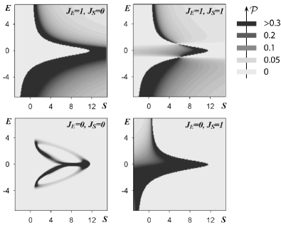
Figure 4: Steady-state probability distribution as function of the radiation strength $E$ and the difference of level populations $S$ at conditions $\tau_{P}\ll\tau_{E}=\tau_{S}$ for parameters $\kappa=10$, $S_{e}=11.6$, $g_{E}=0.2$, $g_{P}=0.2$, $g_{S}=0.2$ and different probability currents $J_{0}^{(E)}$, $J_{0}^{(S)}$ (shown on the related panels)

probability distribution function on the limit cycle of variation of the radiation strength $E$ and the difference of level populations $S$ at zeros probability currents $J_{0}^{(E)}$ and $J_{0}^{(S)}$ only. With increase of these currents the system escapes from equilibrium steady state and maximum of the distribution function shifts to non-closed curves being determined with equation (IV).

V Conclusion

We have considered effect of stochastic sources upon self-organization process being initiated with creation of the limit cycle induced by the Hopf bifurcation. In Sections III–IV, we have applied general relations obtained in Section II to the stochastic Lorenz system to show that departure from equilibrium steady state can destroy or create the limit cycle in dependence of relation between characteristic scales of temporal variation of principle variables.

Investigation of the Lorenz system with different regimes of principle variables slaving shows that additive noises can take multiplicative character if one of these noises has many fewer time scale than others. In such a case, the limit cycle may be created if the most fast variable is coupled with more than two slow ones. However, the case considered in Section IV shows such dependence is not necessarily to arrive at limit cycle, as within adiabatic condition $\tau_{P}\ll\tau_{E}$, both noise amplitude $G_{S}(E)$ and generalized force $\mathcal{F}^{(S)}(E)$, determined with Eqs. (24), (IV), are functions of the squared strength $E^{2}$ only. The limit cycle is created if the fastest variations displays a principle variable, which is coupled with two different degrees of freedom or more. Indeed, at the relation $\tau_{E}\ll\tau_{P},\tau_{S}$ of relaxation times considered in Section III, variations of the strength $E$ in nonlinear terms of two last equations (III) arrive at double-valued dependencies of the noise amplitudes $G_{P}$ and $G_{S}$ on both difference of level populations and polarization, which are appeared in Eqs.(19) as squares $S^{2}$ and $P^{2}$. This appears physically as noise induced resonance related to the limit cycle created by the Hopf bifurcation, that has been observed both numerically d and analytically 26 .

References

• (1) Moss F and McClintock P V E 1989 Noise in Nonlinear Dynamical Systems (Cambridge: Cambridge University Press)
• (2) Horsthemke H and Lefever R 1984 Noise Induced Transitions (Berlin: Springer-Verlag)
• (3) Reimann P, 2002 Phys. Rep. 361 57
• (4) Van den Broeck C, Parrondo J M R and Toral R, 1994 Phys. Rev. Lett. 73 3395; Van den Broeck C, Parrondo J M R, Armero J and Hernndez-Machado A 1994, Phys. Rev. E 49 2639
• (5) Olemskoi A I, Kharchenko D O and Knyaz’ I A, 2005 Phys. Rev. E 71 041101(12)
• (6) Benzi R, Sutera A and Vulpiani A, 1981 J. Phys. A 14 L453
• (7) Gammaitoni L, HΓ€nggi P, Jung P and Marchesoni F, 1998 Rev. Mod. Phys. 70 223
• (8) Buceta J, Ibaes M, Sancho J M and Katja Lindenberg, 2003 Phys. Rev. E 67 021113
• (9) Cross M C and Hohenberg P C, 1993 Rev. Mod. Phys. 65 851
• (10) Julicher F, Ajdari A and Prost J, 1997 Rev. Mod. Phys. 69 1269
• (11) Kautz R L, 1985 J. Appl. Phys. 58 424
• (12) Arecchi F, Badii R and Politi A, 1985 Phys. Rev. A 32 402
• (13) Gao J B, Wen-wen Tung and Nageswara Rao, 2002 Phys. Rev. Lett. 89 254101
• (14) Omar Osenda, Carlos B Briozzo and Manuel O Caceres, 1997 Phys. Rev. E 55 R3824
• (15) Alonso D, McKane A J and Pascual M, 2007 J. R. Soc. Interface 4 575
• (16) Simoes M, Telo da Gama M M and Nunes A, 2008 J. R. Soc. Interface 5 555
• (17) Kuske R, Gordillo L F and Greenwood P, 2007 J. Theor. Biol. 245 459
• (18) McKane A J and Newman T J, 2005 Phys. Rev. Lett. 94 218102
• (19) Pineda-Krch M, Blok H J, Dieckmann U and Doebeli M, 2007 Oikos 116 53
• (20) M S de la Lama, Szendro I G, Iglesias J R and Wio H S, 2006 Eur. Phys. J. B 51 435
• (21) Gonze D, Halloy J and Gaspard P, 2002 J. Chem. Phys. 116 10997
• (22) McKane A J, Nagy J D, Newman T J and Stefanini M O, 2007 J. Stat. Phys. 128 165
• (23) Scott M, Ingalls B and Kaern M, 2006 Chaos 16 026107
• (24) Ben-Naim E and Krapivsky P L, 2004 Phys. Rev. E 69 046113
• (25) Hassard B D, Kazarinoff N D and Wan Y-H 1981 Theory and Applications of Hopf Bifurcation (Cambridge: Cambridge University Press)
• (26) Grimshaw R 1990 Nonlinear Ordinary Differential Equations (Oxford: Blackwell)
• (27) Bartlett M S, 1957 J. R. Stat. Soc. A 120 48
• (28) McKane A J and Newman T J, 2005 Phys. Rev. Let. 94 218102
• (29) Boland R P, Galla T and McKane A J, arXiv:cond-mat 0805.1607
• (30) Haken H 1983 Synergetics (Berlin: Springer-Verlag)
• (31) Lorenz E, 1963 J. Atmosph. Sc. 20 1675
• (32) Risken H 1984 The Fokker-Planck Equation (Berlin: Springer-Verlag)
• (33) N G van Kampen 1990 Stochastic process in physics and chemistry (Amsterdam: North-Holland)
• (34) Olemskoi A I, Kharchenko D O and Kharchenko V O, 2006 Sumy Sate Univ. Bull. No.1 75
• (35) Himadri, Samanta S and Bhattacharjee J K, arXiv:cond-mat 0808.3956