Lawn tennis balls, Rolling friction experiment and Trouton viscosity

Abstract

We took three lawn tennis balls arbitrarily. One was moderately old, one was old and another was new. Fabricating a conveyor belt set-up we have measured rolling friction coefficients, $\mu_{r}$, of the three balls as a function of their angular velocities, $\omega_{ball}$. In all the three cases, plotting the results and using linear fits, we have obtained relations of the form $\mu_{r}=k_{rol}\omega_{ball}$ and have deduced the proportionality constant $k_{rol}$. Moreover, core of a lawn tennis ball is made of vulcanised India-rubber. Using the known values of Young modulus and shear viscosity of vulcanised India-rubbers in the theoretical formula for $k_{rol}$, we estimate $k_{rol}$s for the cores made of vulcanised India-rubbers, assuming Trouton ratio as three. The experimental results for the balls and the semi-theoretical estimates for the cores, of $k_{rol}$, are of the same order of magnitudes.

I Introduction

The game of tennis or, lawn-tennis as it’s known nowadays, has an interesting history. Even the balls [1, 2] used in the game also enjoys an equally interesting story. A ball consists of two parts. The core is made of vulcanised India-rubber[3], whereas, the cover is made of seamless fabric, composed of wool and artificial fiber. The ball has evolved through time and today all balls come in yellow colour.

We randomly took three lawn tennis balls. One was moderately old, after having been played. Another was old, wool was almost not there. The third ball was brand new. Primary objective was to do a rolling friction experiment. Main motivation behind, was to do phenomenology, namely check the formula of Brilliantov et.al.[4], relating rolling friction coefficient with angular velocity. We embark on measuring rolling friction coefficient of these three balls with the instrument we made, following Ko. et.al.[5]. Ko. et.al. developed their working principle of measurement, assuming the presence of rolling friction. They did it keeping the linear result of Brilliantov et.al.[4] on bulk rolling friction, in mind.

Friction is something that always resists the motion of any object. Friction is of mainly three types-static, sliding and rolling. While static and sliding frictions are forces, mainly due to surface effects and act through the point of contact of two bodies, rolling friction is predominantly a bulk effect[4], with very little effect, arising from the surface of contact. Unlike the other two, rolling friction is a couple. It opposes rotational motion only. It is due to hysteresis loss during repeated cycles of deformation and recovery of the body undergoing rolling. Rolling friction mainly depends upon four parameters. These are mechanical properties of the body, radius of the rolling object, nature of the ground and the forward speed respectively. Mechanical properties involved are elastic constants and viscosity coefficients.

The measurement of rolling friction, in general, follows the following recent story. In a paper by Domenech et.al.[6], it was found that the coefficient of rolling friction of a ball rolling up an incline is dependent on the radius of the ball. To measure the speed dependent coefficient of rolling friction, Edmonds et.al.[7] constructed a set up analogous to a cyclotron used to accelerate protons. However, the measurements require the availability of relevant data such as frictions at different joints and the relation between the coefficient of rolling friction and the speed of the ball. Soodak and Tiersten[8] used the perturbation method to analyze effects of rolling friction on the path of a rolling ball on a spinning turntable. Similar effects were also analysed by Ehrlich and Tuszynski[9] who proposed to measure the coefficient of rolling friction of the ball when it starts to rotate, using an inclined mirror. The coefficient of rolling friction was found to be tangent of the angle of inclination. Budinski[10] used the similar method to measure the break away coefficient of rolling friction for rolling element bearings.
The set-up proposed by Y. Xu, K. L. Yung and S. M. Ko[5], in particular, consists of a wood plate and a plastic frame. The plastic frame was mounted around the belt to keep the ball in place. The conveyor belt and the motor were fixed on the wood plate of which one end was supported by the jack. The angle of inclination of the belt was varied by changing the height of the jack. Rotational speed of the squash ball used, was between twenty to forty rpm. They got the value of $k_{rol}$ as $0.0005$ minutes while the full relation obtained experimentally was $\mu_{r}(\omega)=0.0005\omega+0.0092$ with linear regression coefficient $0.96734$.
This paper is organised as follows. In the section II, we describe our setup and the working principle behind our measurement. In the section III, we develop the theoretical background required to interpret our experimental results. In the next section IV, we describe our experiment and our observations with analysis. In the section V. we compare our experimental results with that deduced semi-theoretically, followed by a discussion on different issues and possibilities arising out of the experiment.

II Experimental Setup and Working Principle

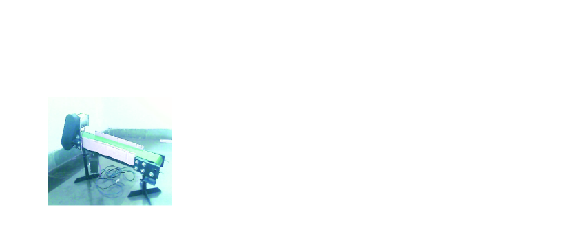
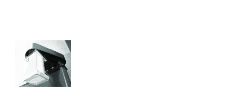
Figure 1: Conveyor belt set-up

Figure 2: DC motor of the set-up

The conveyor belt setup was made of steel to provide stability at higher rpms of the motor. The motor was connected to the rollers of the belt using a gear chain arrangement. The motor was also provided with an electric dimmer to vary the rotational speed of the motor. The conveyor belt was mounted on stands of variable heights on either end to facilitate variation in the angle of the inclined surface of the belt. The belt was 12.7 cm wide and 140 cm long. The diameters of the rollers of the conveyor belt were 4.36 cm. In place of the hollow sphere, tennis balls of varied texture, age and weight were used. Temperature conditions of $32^{0}$C, high humidity and negligible wind conditions were maintained throughout the experiment.
The conveyor belt assembly consists of a dc motor and an electrical setup for converting ac supply voltage to the required dc voltage. The dc motor is of 0.25 hp and peak speed of around 150 rpm.

Fig.3 depicts a viscoelastic sphere of radius $r$ rolling down an incline of angle $\beta$.

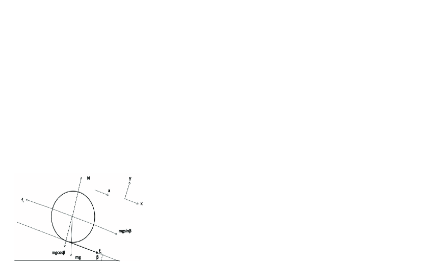
Figure 3: a viscoelastic sphere rolling down a hard incline

Here, $mg$ is the weight of the body, $f_{s}$ is the sliding friction force plus $f_{r}$, where, $f_{r}$ is the rolling friction force, $a$ is the acceleration of the sphere with respect to the ground, along the incline. We recall that the rolling friction is a couple. Assuming the co-ordinate axis as shown in the Fig.3, and applying Newton’s second law along the incline, we get

$$ma=mgsin\beta+f_{s}-f_{r}$$ (1)

and normal to the axis we get

$$N=mgcos\beta$$ (2)

Taking torque about the center of the sphere, we get

$$\tau=rf_{s}$$ (3)

where $\tau$ is the net torque. But we know that torque of a body can be written as

$$\tau=I\alpha$$ (4)

where $I$ is the moment of inertia of the body and $\alpha$ is the angular acceleration of the body w.r.t its center of mass. Equating the two equations(3,4), we get

$$I\alpha=rf_{s}$$ (5)

or,

$$f_{s}=\frac{I\alpha}{r}$$ (6)

For rolling,

$$v=r\omega_{ball}$$ (7)

Equivalently this is

$$a=r\alpha$$ (8)

Substituting this in the eq.(6), we get

$$f_{s}=\frac{Ia}{r^{2}}$$ (9)

Combining eq.(9) with the eq.(1) one gets

$$ma=mgsin\beta+\frac{Ia}{r^{2}}-f_{r}$$

$$ma-\frac{Ia}{r^{2}}=mgsin\beta-f_{r}$$

$$(m-\frac{I}{r^{2}})a=mgsin\beta-f_{r}$$ (10)

For the ball that we used, the value of $I$ lies between that of a hollow sphere with a thin shell and that of a solid sphere. Therefore the term in the brackets in the eq.(II) can never be zero. Hence, eq.(II) determines the acceleration of the ball with respect to the ground when it’s rolling down or, rolling up or, remaining stationary as the conveyor belt beneath moves up. In the particular case, when it’s remaining in one position with respect to the ground, acceleration is zero, leading to

$$mgsin\beta-f_{r}=0$$ (11)

or,

$$f_{r}=mgsin\beta.$$ (12)

Following usual convention,

$$f_{r}=\mu_{r}N$$ (13)

where, $N$ is the normal reaction of the plane on the ball. From the eqns.(2) and (13), we get

$$f_{r}=\mu_{r}mgcos\beta$$ (14)

From the eqns.(12) and (14), we get

$$\mu_{r}=tan\beta.$$ (15)

This equation(15) is the basis of our experiment.

III Theoretical Prelude

Moreover,

$$\mu_{r}=k_{rol}\omega_{ball}.$$ (16)

This expression(16) relating the coefficient of rolling friction and the angular speed of a viscoelastic ball rolling on a hard plane, as shown in the Fig.3, was first derived in 1996. The result was derived basing on the celebrated Hertz contact problem [11, 12], taking only rolling friction loss due to the bulk into account. It was found that this relation is linear for low velocities compared to the velocity of sound in the body. The linearity prevails as long as the characteristic time of the deformation process is much larger than the dissipative relaxation time of the material. It was also found that

$$k_{rol}=\frac{1}{3}\frac{(3\eta_{2}-\eta_{1})^{2}}{(3\eta_{2}+2\eta_{1})}\frac{(3E_{2}+2E_{1})}{(3E_{2}-E_{1})^{2}}.$$ (17)

with $k_{rol}$ carrying the dimension of time. $E_{2}$ and $\eta_{2}$ are the bulk elasticity and viscosity, whereas, $\frac{E_{1}}{2}$ and $\frac{\eta_{1}}{2}$ are shear moduli of elasticity and viscosity respectively, as per the conventions in [13], [14].
We apply eq.(17) to find out $k_{rol}$ for the core of the three lawn tennis balls. Since we do not have any knowledge about the specific type of vulcanised India-rubber, we instead compute $k_{rol}$ for the three kinds of vulcanised India-rubber dealt in [14]. India-rubber, chemically, is a polymer called Polyterpin. Vulcanisation introduces sulphur bridges connecting different polymer chains. According to the content of the sulfur, India-rubber gets different hue. If it contains 2.1 percent sulphur, it appears red. It looks hard grey, if the sulphur content is 3.8 percent. If it contains 5.7 percent sulphur, it’s colour is soft grey [14]. Viscoelasticity datas about these three kinds of rubber are also available in [14].

To do the estimation, we simplify the expression for $k_{rol}$. Moreover, we note that for an isotropic material only two elastic constants and only two viscosity coefficients are independent[13, 12]. These are shear and bulk moduli. On the top of it, if we assume isotropy of relaxation-time, $E_{2}$ and $\eta_{2}$ have got the similar formal expressions,

$$E_{2}=\frac{Y}{3(1-2\sigma)},\eta_{2}=\frac{\overline{\eta}}{3(1-2\sigma)}.$$ (18)

Expressions for $\frac{E_{1}}{2}$ and $\frac{\eta_{1}}{2}$ are also exactly similar,

$$\frac{E_{1}}{2}=\frac{Y}{2(1+\sigma)},\frac{\eta_{1}}{2}=\frac{\overline{\eta}}{2(1+\sigma)}$$ (19)

It happens so that the relatively less discussed of all these moduli is the Trouton viscosity[15, 16], $\overline{\eta}$, with the following definition,

$$\overline{\eta}=\frac{\frac{F}{A}}{\frac{dv_{x}}{dx}}$$ (20)

for a viscoelastic rod with area A, applied force F, longitudinal velocity, $v_{x}$, at a position $x$. We recall for the same rod, Young’s modulus is as

$$Y=\frac{\frac{F}{A}}{\frac{du_{x}}{dx}},$$ (21)

where,

$$v_{x}=\frac{du_{x}}{dt}.$$ (22)

On using the eqns.(18,19), the expression(17) reduces to

$$k_{rol}=\frac{\overline{\eta}}{Y}.$$ (23)

As the bulk viscosity of the vulcanised rubber [14], is very high, Young’s modulus, $Y$, is almost three times that of shear elasticity, $\frac{E_{1}}{2}$. Hence, the Trouton viscosity, $\overline{\eta}$, is approximately three times[15] that of shear viscosity $\frac{\eta_{1}}{2}$. In other words, Trouton ratio is three[16]. As a result, the final expression of $k_{rol}$ for vulcanised rubber is

$$k_{rol}=\frac{3\eta_{1}}{2Y}.$$ (24)

Noting down the experimentally determined values of $\frac{\eta_{1}}{2}$ and $Y$, from the reference[14], and using the relation(24), $\mathbf{k_{rol}}$ for the viscoelastic spheres made of the three kind of rubbers, are found as

$$\mathbf{k_{rol}^{red}}=\mathbf{0.036s},\mathbf{k_{rol}^{softgrey}}=\mathbf{0.212s},k_{rol}^{hardgrey}=0.046s$$ (25)

IV Experiment and Observations

The measurement of velocity dependent coefficient of rolling friction requires the measurement of coefficient of rolling friction at different rotational speeds. The body under observation should undergo pure rotation for measuring the coefficients at different rotational speeds.

When the conveyor belt is moving uphill the ball would have either a tendency to move uphill along with the belt, move downhill in a direction opposite to the motion of the belt or, oscillate between the two extremes (somewhere in the middle may be). In the first case, the ball moves uphill because the rolling frictional force is more than that of gravitation along the incline. Hence we increase the inclination or, reduce the speed. In the second case, the ball moves down as the gravitational force along the incline is more than the rolling frictional force. So we reduce the inclination or, increase the speed. In the third case, the two opposing forces balance each other and hence the ball undergoes an oscillatory motion initially. The ball, due to linear and rotational air drag[17], soon settles down at a fixed point w.r.t the ground, making rotation at constant angular velocity and we get the desired reading. Due to rolling friction’s dissipative role, albeit little, the ball looses angular velocity and hence looses the rolling frictional force keeping it balanced against gravity and after a little while goes down along the conveyor belt.

The conveyor belt is set at different angles of inclination. For each angle, the motor is started at the minimum possible speed and the ball is placed on the belt. Depending on its direction of motion, the speed of the belt is regulated so as to achieve zero translational velocity of the ball with respect to the ground. At such a condition, the angle of inclination of the belt, $\beta$, and the apparent angular velocity of the ball, $\omega$, is measured in the following way. The rotational speed of the rollers was measured using a tachometer. The apparent angular velocity of the ball is then calculated by dividing the value of the linear velocity of the belt by the value of the radius of the tennis ball. Moreover, the linear velocity of the belt is calculated by multiplying the radius of a roller with its rpm. Hence,

$$\omega=\frac{\omega_{conveyor}r_{roller}}{r_{ball}}$$ (26)

The ball is ”quasirolling” [18] as little skidding unavoidably comes with pure rolling. The speed of the conveyor belt is slightly higher by $v_{skid}$ relative to the speed of the instantaneous point of contact on the ball. As a result,

$$\omega_{ball}=\omega-\frac{v_{skid}}{r_{ball}}.$$ (27)

The measurement of the angle of the incline is done in a very simplified way. The whole setup can be assumed to be a right angled triangle with its hypotenuse representing a straight line between the two rollers on which the conveyor belt runs. The length of the hypotenuse was calculated by measuring the distance between the centers of the two pulleys, using a meter scale and a Vernier Callipers. The height of the right angled triangle can be easily estimated by measuring the heights of the centers of both the rollers and then taking their difference.

The above procedure is followed for a number of readings. A graph is then plotted using Matlab between $\mu_{r}$, and the apparent rotational speed of the ball, $\omega$, utilising eq.(15). The same steps are repeated for the other two balls.

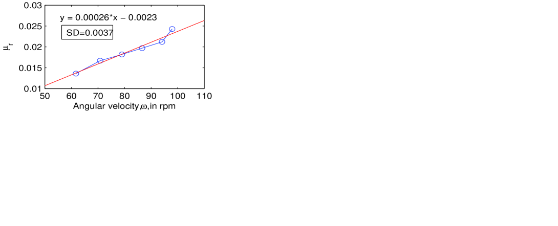
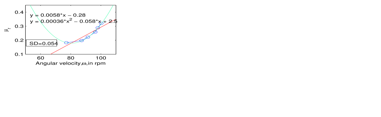
Figure 4: Graphs for a moderately old ball, $R^{2}=1$; an old ball, $R^{2}=0.964$; a new lawn tennis ball, $R^{2}=0.821$

It’s seen that graphs are almost linear, with negative intercepts, as expected from the eqns.(15, 16, 27). In case of the new ball, due to the predominant presence of felt, slipping, $v_{skid}$, quite likely have been different for different speeds of the conveyor belt, giving rise to the apparent quadratic nature of the plot. However, a linear relationship is obtained in each case through least square regression. The regression coefficient $R^{2}$ noted in the captions of the graphs is the square of correlation coefficient between the $\mu_{r}$ values observed and values on the best-fit,

$$R^{2}=1-\frac{\sum{(y_{i}-f_{i})^{2}}}{\sum{(y_{i}-\overline{y})^{2}}},$$ (28)

where, $f_{i}$ are values on the best-fit straight line, at the i-th position, $i=1,..,5or,6$. Value of $R^{2}$ shows that for the new ball even linear fit is good.

tennis balls	relation between $\mu_{r}$ and	Hence,
	$\omega$(in rpm)	$\mathbf{k_{rol}}$
(ages)	$\mu_{r}=k_{rol}\omega-const$	(in min)
moderately	$\mu_{r}=0.00042\omega-0.0190$	0.00042
old
old	$\mu_{r}=0.00026\omega-0.0023$	0.00026
new	$\mu_{r}=0.00580\omega-0.2800$	0.00580

Table 1: Facts obtained from graphs, on experimental results, for balls of different ages.

Table 1 enlists the linear relations, thereof, case by case. Hence, $k_{rol}$, determined from our rolling friction experiment, but expressed in seconds, are as

$$\mathbf{k_{rol}^{moderatelyold}}=\mathbf{0.025s},\mathbf{k_{rol}^{old}}=\mathbf{0.016s},k_{rol}^{new}=0.348s.$$ (29)

V Discussion

Comparing $R^{2}$ for the best-fit lines in the three graphs, we notice that linear fit is most accurate in the case of the moderately old ball. We see that $k_{rol}$ calculated for red-grey rubber is also closest to $k_{rol}$ inferred from the second graph. Moreover, on matching the relations(25) and (29), we observe that $k_{rol}$ for the moderately old ball/ old ball is too close to that of red grey India-rubber, whereas $k_{rol}$ for the new ball is close to the soft-grey India-rubber. These lead us to conclude the following three possibilities, a) moderately old ball/old ball, we have used had the core made up of red grey India-rubber and the new ball had the core made up of soft-grey India-rubber; b) all the balls were having the core made up of soft-grey India-rubber. With mechanical degradation associated with shots, $\overline{\eta}$ and $Y$ got reduced thus reducing $k_{rol}$ and the moderately old ball/old ball behaving like having core made up of red-grey India-rubber; c)all the balls used by us were having core made up of red-grey India-rubber and for the new ball, predominant contribution is due to felt.
We have used balls, available in local market. Most likely, those were trainer balls made not following ITF specifications fully. Moreover, ITF ball specification points to [1] vulcanised red-grey India-rubber as the core material. In future, we plan to take a full investigation with ITF approved professional balls, along the line of this paper.
In principle, rolling friction due to surface interaction should be taken into account. One can include rotational air drag also. The side of the ball coming down to onto the conveyor belt has lower pressure head in the adjoining air volume, compared to the other side. This leads to a drag force, working opposite to $f_{r}$ shown in the Fig.3. In that case we would have gotten the same eq.(15) with R.H.S. of the eq.(16) getting modified by the additional presence of rotational terms and surface rolling friction terms.
One limitation of this setup in this present form that it requires at least five persons to do the experiment. The most time consuming step of the experiment was the angle adjustment step of the conveyor belt. We have taken each reading twice, due to limited availability of tachometer. We are pretty sure about the repeatability.
We have not used anything to reduce air hindrance, by putting a plastic frame, say as in Ko et.al’s[5] experiment. Fabrication of our setup has cost us approximately $250$ USD. The motor being a 150 rpm motor, we could achieve only limited ball angular velocity. It would be interesting to get DC motors of different hps, custom-made, and achieve higher speeds for the conveyor belt and thereby get rolling friction coefficient, at non-linear angular velocity regime[19, 20, 2], checked for different objects.
However, the relation,

$$\overline{\eta}=k_{rol}Y,$$ (30)

leads us to an almost direct way of measuring Trouton viscosity of a viscoelastic substance. Only thing we need to know as an input from outside, the Young modulus, $Y$. Hence, the setup which we are using to measure $k_{rol}$ directly, can be used to determine, in addition, Trouton viscosity of a viscoelastic material.

VI Acknowledgement

We would like to thank G. J. Desai, V. V. Chaudhari and P. R. Dhimaan for helping us design the set up, Harshit Khurana for his comments on the manuscript and the Electrical Department Lab personnel of BITS-GOA, for lending us a tachometer. We are grateful to the anonymous Referees for their invaluable suggestions.

References

- [1] www.itftennis.com/technical/rules/history/index.asp
- [2] R. D. Mehta, ” Aerodynamics of Sports Balls”, Ann. Rev. Fluid Mech. 1985. 17: 151-89; J. M. Zayas, ” Experimental determination of the coefficient of drag of a tennis ball”, Am. J. Phys. 54(7), 622-625(1986); R. G. Watts and R. Ferrer, ” The lateral force on a spinning sphere: Aerodynamics of a curveball”, Am. J. Phys. 55(1), 40-44(1987); A. Stepanek, ” The aerodynamics of tennis balls-The topspin lob”, Am. J. Phys. 56(2), 138-142(1988); R. D. Mehta and J. M. Pallis, ”The aerodynamics of a tennis ball”, Sports Engineering (2001)4, 177-189; S. R. Goodwill, S. B. Chin, S. J. Haake, ”Aerodynamics of spinning and non-spinning tennis balls”, Journal of Wind engineering and Industrial Aerodynamics 92 (2004) 953-958; R. D. Mehta, F. Alam and A. Subic, ”Review of tennis ball aerodynamics”, Sports Technol. 2008,1, No. 1, 7-16; C. Steele, R. Jones, P. leaney, ”Improved tennis ball design: incorporating mechanical and psychological influences,” Journal Of Engineering Design. 19(3), 269-284(2008) and references therein.
- [3] www.henriettesherbal.com/eclectic/kings/hevea.html
- [4] N. V. Brilliantov and T. Poschel, ”Rolling friction of a viscous sphere on a hard plane,” Europhys. Lett.42, 511-16(1998)
- [5] Y. Xu, K. L. Yung and S. M. Ko, ”A classroom experiment to measure the speed-dependent coefficient of rolling friction,” Am. J. Phys. 75(6), 571-74(2007).
- [6] A. Domenech, T. Domenech and J. Cebrian, ”Introduction to the study of rolling friction,” Am. J. Phys. 55, 231-235(1987)
- [7] L. Edmonds, N. Giannakis and C. Henderson, ”Cyclotron analog applied to the measurement of rolling friction,” Am. J.Phys. 63, 76-80(1995).
- [8] H. Soodak and M. S. Tiersten, ”Perturbation analysis of rolling friction on a turntable,” Am. J. Phys. 64, 1130-39(1996).
- [9] R. Ehrlich and J. Tuszynski, ”Ball on a rotating turntable: Comparison of theory and experiment,” Am. J. Phys. 63, 351-59(1995).
- [10] K. G. Budinski, ”An incline plane test for the breakaway coefficient of rolling friction of rolling element bearings,” Wear 259, 1443-47(2005).
- [11] H. Hertz, J. f. reine u. angewandte Math. 92, 156(1882).
- [12] L. D. Landau and E. M. Lifshitz, Theory of Elasticity (Pergamon Press, London, 1959).
- [13] R. P. Feynman, R. B. Leighton, M. Sands, The Feynman Lectures On Physics, Vol 2, (Narosa Publishing, 1986, New Delhi).
- [14] A. Mallock, ”The Physical Properties Of Vulcanised India-Rubber,” Proc. Roy. Soc. 46, 233-249(1889).
- [15] F. A. Morrison, Understanding Rheology (Oxford Univ. Press, Inc. 2001), p214.
- [16] F. T. Trouton, ”On the Coefficient of Viscous Traction and Its Relation to that of Viscosity,” Proc. Roy. Soc. A 77, 426(1906).
- [17] B. G. Thompson and P. A. Smith, ”An experiment in rotational motion with linear and quadratic drag,” Am. J. Phys. 72, 839-42(2004)
- [18] N. Sharma and D. D. Reid, ”Rolling as a frictional equilibration of translation and rotation”, Europhys. Journal.20, 129-136(1999)pp132
- [19] Y. Xu and K. L. Yung, ” The effect of inertial normal force on the rolling friction of a soft sphere on a hard plane”, Europhys. Lett.61, 620-24(2003)
- [20] Y. Xu and K. L. Yung, ” Non-Linear Expressions for Rolling Friction of a Soft Ball on a Hard plane”, Nonlinear Dynamics 33, 33-41(2003).