Large deviations for the leaves in some random trees

Abstract.

Large deviation principles and related results are given for a class of Markov chains associated to the “leaves” in random recursive trees and preferential attachment random graphs, as well as the “cherries” in Yule trees. In particular, the method of proof, combining analytic and Dupuis-Ellis type path arguments, allows for an explicit computation of the large deviation pressure.

1. Introduction and results

We consider in this article large deviations and related laws of large numbers and central limit theorems for a class of Markov chains associated to the number of leaves, or nodes of degree one, in preferential attachment random graphs and random recursive trees, and also the number of “cherries,” or pairs of leaves with a common parent, in Yule trees. The random graphs studied model various networks such as pyramid schemes, chemical polymerization, the internet, social structures, genealogical families, among others. In particular, the leaf and cherry counts in these models are of interest, and have concrete interpretations. In Subsection 1.2, we discuss applications with these models and literature.

Define the nondecreasing Markov chain $\{Z_{n}:n\geq 1\}$ starting from initial state $Z_{1}=k_{0}\geq 0$, by its one-step transitions, for $n\geq 1$,

(1.1) $$\Pr\big{(}Z_{n+1}-Z_{n}=v|Z_{n}\big{)}\ =\ \begin{cases}1-\frac{Z_{n}}{s_{n}}&\mbox{ if $v=1$}\\ \frac{Z_{n}}{s_{n}}&\mbox{ if $v=0$}\\ \end{cases}$$

where $\{s_{n}:n\geq 1\}$ is a sequence of positive numbers such that

(1.2) $$s_{n}\geq k_{0}+n-1,\mbox{ and }\frac{s_{n}}{n}\rightarrow\alpha\mbox{ for }1<\alpha<\infty$$

with convention $0/0=0$. Additionally, we also consider two special sequences, $s_{n}=n$ and $s_{n}=n/2$ with $k_{0}\leq s_{1}$, related to some applications.

We first note, in this form, $Z_{n}$ can be seen to represent the “mass” of red balls in a Polya-Eggenberger-type urn of two colors, red and blue, not necessarily tenable, where at each time $n$, proportional to the red balls mass, a (signed) mass $s_{n+1}-s_{n}$ of blue balls is deposited, otherwise one red ball and mass $s_{n+1}-s_{n}-1$ of blue balls is added.

Also, when $s_{n}=(k_{0}+2(n-1)+n\beta)/(1+\beta)$ and $\alpha=(2+\beta)/(1+\beta)$ for $\beta>-1$, the chain has interpretation as the number of leaves in preferential attachment random graphs with weight function $f(k)=k+\beta$. Later, in Subsection 1.2, we also remark that $s_{n}$ can be taken as a random sequence with respect to the number of “generalized” leaves, or “buds,” that is those nodes, possibly with degree greater than one, which however connect to only one other vertex, in preferential attachment graphs with random edge additions.

In addition, when $s_{n}=\alpha n$ for $\alpha=1,2$, $Z_{n}$ is also the number of leaves in uniformly and planar oriented recursive trees respectively. In the latter case $\alpha=2$, $Z_{n}$ is also the number of “plateaux” in a random Stirling permutation of length $2n$.

Moreover, when $s_{n}=n/2$, $Z_{n}$ can be seen as the number of cherries in Yule trees.

As the urns add mass of the opposite color, one should expect almost sure limits for the mean behavior and Normal fluctuations. In fact, by mostly martingale, combinatorial and urn methods, laws of large numbers (LLN) and central limit theorems (CLT) have been proved, at least in the examples mentioned above when $s_{n}$ is linear with slope $\alpha$ (cf. Theorem 1.4). See [9, 36, 40] with respect to preferential attachment, [28], [41] with respect to recursive trees, [34] with respect to Yule trees, and [33] with respect to urns when $\alpha$ is a positive integer.

Characterizing the associated large deviations is a natural problem which gives insight into the properties of rare events, and seems less studied in urns or random graphs. Previous work has concentrated on analytic methods with respect to “subtraction” urn models–not applicable in our general setting [24]–or extensions of the Dupuis-Ellis weak convergence approach (cf. [20]) to different allocation models than ours [21], [44]. We note also some exponential bounds via martingale concentration inequalities are found in the case $s_{n}$ is linear with slope $\alpha$ [15]. See also [4, 6, 12, 17, 19, 27] for other types of large deviations work in various random tree models.

In this context, our main results are to prove a large deviation principle (LDP) for $Z_{n}/n$ with an explicitly computed “pressure,” or Legendre transform of the associated rate function (Theorem 1.1). This is done in two different ways for the important case $s_{n}$ is linear with $\alpha=2$. Such explicit computations are not commonplace, and our “ODE” method is quite different from the methods in [24] where a quasi-linear PDE is solved, or in [44] where a finite-dimensional minimization problem is obtained.

Perhaps a main feature of our work is that the method given appears robust and applicable in diverse, not necessarily urn settings. In particular, we show the LDP for $Z_{n}/n$ does not feel the disorder in the sequence $s_{n}$, is not dependent on the initial value $Z_{1}$, and is the same as for the chain with a regular, linear $s_{n}$ with slope $\alpha$. We mention that this is a consequence of a large deviation principle for the path interpolation of $Z_{\lfloor nt\rfloor}/n$ (Theorem 1.3), perhaps of interest in itself, that we establish, by the Dupuis-Ellis weak convergence approach.

In addition, aside from laws of large numbers which are trivially obtained, we prove a central limit theorem for $Z_{n}$ through complex variables arguments with the pressure (Theorem 1.4). These alternate proofs of the LLN and CLT, although indirect, apply when the mass additions take on some negative non-integer values where less is known in the literature. Moreover, the results give a “quenched” LLN, CLT and LDP’s with respect to “generalized” leaves or buds in a preferential attachment scheme with random edge additions (see Subsection 1.2).

Our technique to prove the LDP for $Z_{n}/n$ is to consider the recurrence relation for $m_{n}(\lambda)=E[\exp\{\lambda Z_{n}\}]$ obtained from (1.1):

(1.3) $$m_{n+1}(\lambda)\ =\ ({1-e^{\lambda}})\frac{m^{\prime}_{n}(\lambda)}{s_{n}}+e^{\lambda}m_{n}(\lambda).$$

Dividing through by $m_{n}(\lambda)$, we write

(1.4) $$\frac{m_{n+1}(\lambda)}{m_{n}(\lambda)}\ =\ \frac{1-e^{\lambda}}{s_{n}/n}\frac{m^{\prime}_{n}(\lambda)}{nm_{n}(\lambda)}+e^{\lambda}.$$

The idea now is to take the limit on $n$ in the above display. When the “pressure” $\Lambda$ exists, it satisfies $\Lambda(\lambda)=\lim_{n\rightarrow\infty}(1/n)\log m_{n}(\lambda)$. In this case, it is natural to suppose that the limits

(1.5) $$\Lambda^{\prime}(\lambda) = \lim_{n\rightarrow\infty}\frac{m_{n}^{\prime}(\lambda)}{nm_{n}(\lambda)}$$

(1.6) $$e^{\Lambda(\lambda)} = \lim_{n\rightarrow\infty}\frac{m_{n+1}(\lambda)}{m_{n}(\lambda)}$$

both exist. Then, from (1.4), we can write the ODE

(1.7) $$e^{\Lambda(\lambda)}\ =\ \frac{1-e^{\lambda}}{\alpha}\Lambda^{\prime}(\lambda)+e^{\lambda};\ \ \ \Lambda(0)=0.$$

One can compute the solution of this differential equation (cf. (1.12)) and show it is unique.

The main task is to show that the pressure and limits (1.5) and (1.6) exist. But, the pressure exists as a consequence of the path LDP for $Z_{\lfloor nt\rfloor}/n$ by contraction principle. We note, in principle, one can try to compute the pressure or the rate function from (1.13) by the calculus of variations, but we found it difficult to solve the associated Euler equations (cf. near (4.1)).

Finally, we show (1.5) and (1.6) exist by extending $m_{n}(\lambda)$ to the complex plane, and then analyzing its zeroes and analytic properties. These estimates are also useful for the central limit theorem arguments.

We now mention a different approach, in the spirit of [24], when $s_{n}$ is linear with slope $\alpha=2$ and also interestingly $\alpha=1/2,1$, to compute the pressure from analysis of the generating function $G(\lambda,z)=\sum_{n\geq 1}m_{n}(\lambda)z^{n-1}$. From (1.3), we can write the linear PDE

(1.8) $$\frac{\partial G}{\partial z}(1-e^{\lambda}z)+\frac{e^{\lambda}-1}{\alpha}\frac{\partial G}{\partial\lambda}\ =\ e^{\lambda}G.$$

One can solve implicitly this PDE, and locate at least heuristically a singular point. Then, formally, from root test asymptotics, the pressure would be the reciprocal of the location of the singularity.

The difficulty is in establishing the analyticity of the solution and identifying its singularity. For urn models of “subtraction type” where the mass added is an integer, and which satisfies a balance condition, [24] uses this program to obtain large deviations and the CLT. However, the cases $s_{n}$ is linear with slope $\alpha=1/2,1,2$, and more generally the urns associated with non-integer $s_{n}$ are not covered by their arguments which seem to rely on integer additions with a certain “negative” structure. On the other hand, we are able to supply the needed analyticity and singularity identification when $s_{n}$ has slopes $\alpha=1/2,1,2$, and in this way prove the LDP for $Z_{n}/n$ (Theorem 1.1) in these cases.

The plan of the paper is to state the results in Subsection 1.1, discuss applications to random graphs in Subsection 1.2, give the generating function proof of Theorem 1.1 in Section 2, prove the path LDP (Theorem 1.3) in Section 3, give the ODE-method proof of Theorem 1.1 and prove the LLN and CLT (Theorem 1.4) in Section 4, and conclude in Section 5.

1.1. Results

We recall the setting for large deviations. A sequence $\{X_{n}\}$ of random variables with values in a separable complete metric space $\mathbf{X}$ satisfies the large deviation principle (LDP) with speed $n$ and rate function $I:\mathbf{X}\to[0,\infty]$ if $I$ has compact level sets $\{\mathbf{x}:I(\mathbf{x})\leq a\}$, and for every Borel set $U\in\mathcal{B}_{\mathbf{X}}$,

(1.9) $$-\inf_{\mathbf{x}\in U^{\circ}}I(\mathbf{x}) \leq \liminf_{n\to\infty}\frac{1}{n}\log\Pr(X_{n}\in U)$$

$$\leq \limsup_{n\to\infty}\frac{1}{n}\log\Pr(X_{n}\in U)\ \leq\ -\inf_{\mathbf{x}\in\bar{U}}I(\mathbf{x}).$$

[Here $U^{\circ}$ is the interior of $U$ and $\bar{U}$ is the closure of $U$.]

Often the rate function is given in terms of the Legendre transform of the “pressure” when it exists. When $\mathbf{X}=\mathbb{R}$, this representation takes the form

(1.10) $$I(x)\ =\ \sup_{\lambda\in\mathbb{R}}\big{\{}\lambda x-\log\Lambda(\lambda)\big{\}},$$

where we recall the pressure satisfies

(1.11) $$\Lambda(\lambda)\ :=\ \lim_{n\to\infty}\frac{1}{n}\log E[e^{\lambda Z_{n}}].$$

Recall now the Markov chain $Z_{n}$ (1.1) corresponding to sequence $\{s_{n}\}$ and parameter $1<\alpha<\infty$ (1.2).

Theorem 1.1.

The sequence $Z_{n}/n$ satisfies LDP with speed $n$ and good strictly convex rate function $I$ given by (1.10) with pressure

(1.12) $$\Lambda(\lambda)\ =\ -\log\left(\frac{\alpha}{e^{\lambda}-1}\int_{0}^{\lambda}\left(\frac{e^{s}-1}{e^{\lambda}-1}\right)^{\alpha-1}ds\right)\ \ \ \ \ {\rm for\ }\lambda\neq 0$$

and $\Lambda(0)=0$.

Remark 1.2.

We note, when $s_{n}=\alpha n$ with $\alpha=1/2,1$ and $k_{0}\leq s_{1}$, the LDP is also found, with pressure given by formula (1.12), using the generating function approach (cf. Section 2). For $\alpha=1/2$ and integer $\alpha\geq 1$, the integral in (1.12) can be evaluated explicitly.

We now consider the LDP for the family of stochastic processes $\{X_{n}(t):0\leq t\leq 1\}$ obtained by linear interpolation of the Markov chain (1.1),

$$X_{n}(t)\ :=\ \frac{1}{n}Z_{\lfloor nt\rfloor-k_{0}+1}+\frac{nt-\lfloor nt\rfloor}{n}(Z_{\lfloor nt\rfloor-k_{0}+2}-Z_{\lfloor nt\rfloor-k_{0}+1})\ \ {\rm for\ }t\geq\frac{k_{0}}{n}$$

and $X_{n}(t):=t$ for $0\leq t\leq k_{0}/n$. The trajectories of $X_{n}(t)$ are non-decreasing Lipschitz functions with constant at most $1$.

Theorem 1.3.

As a sequence of $C([0,1];\mathbb{R})$-valued random variables, $X_{n}$ satisfies the LDP with the rate function $I:C([0,1];\mathbb{R})\to[0,\infty]$ given by

(1.13) $$I(\varphi)\ =\ \int_{0}^{1}\left[\dot{\varphi}(t)\log\frac{\alpha t\dot{\varphi}(t)}{\alpha t-\varphi(t)}+(1-\dot{\varphi}(t))\log\frac{\alpha t(1-\dot{\varphi}(t))}{\varphi(t)}\right]\,dt$$

if $\varphi(t)$ is differentiable for almost all $t$, $\varphi(0)=0$, $0\leq\dot{\varphi}\leq 1$, and the integral converges; otherwise, $I(\varphi)=\infty$.

By the contraction principle, Theorem 1.3 implies the LDP for $Z_{n}/n$ with the rate function given by the variational expression

(1.14) $$I(x)\ =\ \inf\Big{\{}I(\varphi):\;\varphi(0)=0,\;\varphi(1)=x\Big{\}}.$$

In general, optimal trajectories are not straight lines—exceptions are the LLN trajectory $\varphi_{\alpha}(t)=t\alpha/(\alpha+1)$ and the extreme case $\varphi(t)=t$—but they try to stay near the LLN line (for which $I(\varphi_{\alpha})=0$) to minimize cost before going to destination $x$ (cf. Fig. 1).

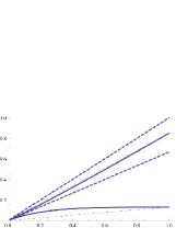
Figure 1. Thick curves are numerical solutions of the Euler equations for (1.14) with $\alpha=2$ for $x=0.13,2/3,0.85,1$. Dashed lines are straight lines from $(0,0)$ to $(1,x)$.

Lemmas for the proof of Theorem 1.1 give Normal approximation. The law of large numbers also follows from Theorem 1.1.

Theorem 1.4.

We have

$$\frac{Z_{n}}{n} \xrightarrow{\rm a.s.} \frac{\alpha}{\alpha+1}$$

and also

$$\frac{1}{\sqrt{n}}(Z_{n}-E[Z_{n}]) \xrightarrow{\rm\;D\;} N(0,\sigma^{2})\ \ \ {\rm where\ \ }\sigma^{2}\ =\ \frac{\alpha^{2}}{(1+\alpha)^{2}(2+\alpha)}.$$

Remark 1.5.

The conclusions of Theorem 1.4 also hold when $s_{n}=\alpha n$ with $\alpha=1/2,1$, and $k_{0}\leq s_{1}$ (cf. Subsection 4.3).

1.2. Applications to random graph models

With respect to random graphs, the Markov chain $Z_{n}$, representing the number of leaves, sits in the intersection of at least two models, that is preferential attachment graphs with linear-type weights, and uniformly and planar oriented trees. Also, when $s_{n}=\alpha n$ for $\alpha=1/2$, $Z_{n}$ represents the count of cherries in Yule trees.

1.2.1. Preferential attachment graphs

Preferential attachment graphs have a long history dating back to Yule (cf. [35]). However, since the work of Barabasi-Albert [1, 5], these graphs have been of recent interest with respect to modeling of various “real-world” networks such as the internet (WWW), and social and biological communities. Leaves, or nodes with degree one, in these networks of course represent sites with one link, or members at the “fringe.” [See books [23], [15], [11] for more discussion.]

The idea is to start with an initial connected graph $G_{1}$ with a finite number of vertices, and say no self-loops (so that the vertices have well-defined degrees). At step $1$, add another vertex, and connect it to a vertex $x$ of $G_{1}$ preferentially, that is with probability proportional to its weight, $f(d_{x})/\sum_{y\in G_{1}}f(d_{y})$, to form a new graph $G_{2}$. Continue in this way by adding a new vertex and connecting it preferentially to form $G_{k}$ for $k\geq 1$. Here, the “weight” of a vertex is a function $f$ of its degree $d_{x}$. When $f:\mathbb{N}\rightarrow\mathcal{R}_{+}$ is increasing, already well connected vertices tend to become better connected, a sort of reinforcing effect.

Our results are applicable to linear weights, $f(k)=k+\beta$, for $\beta>-1$, which correspond to certain “power law” mean degree sequences. Namely, let $Z_{k}(n)$ be the number of vertices in $G_{n}$ with degree $k$ for $k\geq 1$. It was shown, by martingale arguments, in [9], [36], and by embedding into branching processes, in [40] that $Z_{k}(n)/n\rightarrow r_{k}$ a.s. where

$$r_{k}\ =\ \frac{2+\beta}{k+\beta}\prod_{j=1}^{k}\frac{j+\beta}{j+2+2\beta}\ \sim\ 1/k^{3+\beta}.$$

From the applications point of view, the parameter $\beta$ can sometimes be matched to empirical network data where similar power-law behavior is observed.

As the number of vertices with degree $1$, or the “leaves” $Z_{1}(n)$, increases by one in the next step when a non-leaf is selected, and remains the same when a leaf is chosen, we see that $Z_{1}(n)$ corresponds to the Markov chain $Z_{n}$ with $s_{n}$ as specified below. Since at each step the total degree of the graph augments by two, the probability at step $n$ that a vertex $x\in G_{n}$ is selected is $(d_{x}+\beta)/(d_{G_{1}}+2(n-1)+(n-1+|G_{1}|)\beta)$. Then, $s_{n}=\big{(}d_{G_{1}}+2(n-1)+(n-1+|G_{1}|)\beta\big{)}/(1+\beta)$ and $\alpha=(2+\beta)/(1+\beta)$. Here $d_{G_{1}}$ and $|G_{1}|$ are the total degree and number of vertices in $G_{1}$ respectively.

One can also “randomize” the model by adding a random number of edges at each step: Let $\{\gamma_{i}\}$ be a sequence of independent identically distributed random variables on $\mathbb{N}$ with finite mean, $\bar{\gamma}=E[\gamma_{1}]<\infty$. Then, at step $n$, we add a new vertex to the graph $G_{n}$ and connect it to a node selected preferentially from $G_{n}$ with $\gamma_{n}$ edges put between them. The effect of these random edge additions is to randomize further the weight given the nodes in the graph; the “deterministic” model above is when $P(\gamma_{1}=1)\equiv 1$. In [3], by embedding into branching processes, it was shown, when $E(\gamma_{1}\log\gamma_{1})<\infty$, that $Z_{k}(n)/n\stackrel{{\scriptstyle P}}{{\rightarrow}}r_{k}$ where $r_{k}$ is given by an integral formula with asymptotics $r_{k}\sim 1/k^{3+\beta/\bar{\gamma}}$. See [16] for an even more general randomized model where also a LLN is proved. Other models with different random edge addition schemes are found in [19], [31].

In this “randomized” model, we now define the notion of “generalized leaves” or “buds,” that is, those nodes which connect to exactly one other vertex, albeit possibly with several edges linking them. Leaves are those buds with exactly one edge connection. Similar to the leaves in the deterministic setting, at step $n$, the bud count increases by one exactly when the new vertex, a fortiori a bud, connects to a non-bud in $G_{n}$, and remains the same when the new vertex links to a bud in $G_{n}$.

Then, the Markov chain $Z_{n}$, representing the number of buds at step $n$, corresponds to $s_{1}=(d_{G_{1}}+|G_{1}|\beta)/(1+\beta)$ and for $n\geq 2$,

$$s_{n}\ =\ \frac{1}{1+\beta}\Big{[}d_{G_{1}}+2\sum_{i=1}^{n-1}\gamma_{i}+\big{(}n-1+|G_{1}|\big{)}\beta\Big{]},$$

which satisfies assumption (1.2), by the strong law of large numbers, with $\alpha=(2\bar{\gamma}+\beta)/(1+\beta)$ a.s. In particular, by our results, we obtain “quenched” LLN, CLT and LDP’s, with probability one with respect to $\{\gamma_{i}\}$, for the buds in this scheme.

1.2.2. Random recursive trees

Random recursive trees are also well-established models, dating to the 1960’s, with applications to data sorting and searching, pyramid schemes, spread of epidemics, chemical polymerization, family trees (stemma) of copies of ancient manuscripts etc. Leaves in these trees correspond to “shutouts” with respect to pyramid schemes, nodes with small “affinity” in polymerization models, “terminal copies” in stemma of manuscripts etc. See [41], [42] and references therein (e.g. [37] etc.) for more discussion. Below, we mention connections with Stirling permutations.

Similar to preferential attachment, the recursive schemes form a sequence of trees. One starts with a single vertex labeled $0$, and then adds a vertex at step $n\geq 1$, labeled $n$, to one of the $n$ nodes already present. When the choice is made uniformly, the model forms a uniformly recursive tree. However, when the choice is made proportional to the degree, a non-uniform or plane oriented tree is grown. The interpretation is that in uniform trees, at each distance from the root $0$, there is no ordering of the labels. However, in plane-oriented trees, different orders give rise to distinct trees; that is, after selecting a parent node at random at step $n$ with $k$ children with a certain cyclic order of labels, there are $k+1$ locations where the new label $n$ can be inserted.

Plane oriented trees are similar to preferential attachment graphs with $\beta=0$ (cf. Chapter 4 [23]), and the number of leaves corresponds to the Markov chain with $k_{0}=1$, $s_{n}=2n-1$ for $n\geq 1$, and $\alpha=2$. On the other hand, the number of leaves in uniformly recursive trees corresponds to the case $k_{0}=1$, $s_{n}=n$ for $n\geq 1$, and $\alpha=1$. With respect to both types of recursive trees, LLN’s and CLT’s have also been proved by combinatorial, urn and martingale methods (see [41], [28]). So, in this context, our results give alternate proofs of the LLN and CLT for these recursive trees, and also an LDP for $Z_{n}/n$. We note also Theorem 1.3 yields a path LDP for planar oriented trees.

We comment now on recent connections of planar oriented trees with Stirling permutations (cf. [29], [30]). A Stirling permutation of length $2n$ is a permutation of the multiset $\{1,1,2,2,\ldots,n,n\}$ such that for each $i\leq n$ the elements occurring between the two $i$’s are larger than $i$ (cf. [26]). It turns out that each permutation is a distinct code for a plane oriented recursive tree with $n+1$ vertices.

Quoting from [29], consider the depth first walk which starts at the root, and goes first to the leftmost daughter of the root, explores that branch (recursively, using the same rules), returns to the root, and continues to the next daughter and so on. Each edge is passed twice in the walk, once in each direction. Label the edges in the tree according to the order in which they were added–edge $j$ is added at step $j$ and connects vertex $j$ to an previously labeled vertex. The plane recursive tree is coded by the sequence of labels passed by the depth first walk. With respect to a tree with $n+1$ vertices, the code is of length $2n$, where each of the labels $1,2,\ldots,n$ appears twice. Adding a new vertex means inserting the pair $(n+1)(n+1)$ in the code in one of the $2n+1$ places.

In a Stirling permutation $a_{1}a_{2}\cdots a_{2n}$, the index $0\leq i\leq 2n$ is a plateau if $a_{i}=a_{i+1}$ (where $a_{2n+1}=0$). [29] shows that the number of leaves in a plane oriented tree with $n+1$ vertices is the number of plateaux in a random Stirling permutation. See [29] for more details.

1.2.3. Yule trees

Since Yule’s influential 1924 paper [43], Yule trees, among other processes, have been used widely to model phylogenetic evolutionary relationships between species (see [2] for an interesting essay). In particular, the counts of various shapes and features of these trees can be studied, and matched to empirical data to test evolutionary hypotheses. In [34], a LLN and CLT is proved for the number of cherries, or pairs of leaves with a common parent, in Yule trees. Associated confidence intervals are computed, and some empirical data sets are examined to see their compatibility with “Yule tree” genealogies. Other related statistical tests and limit results can be found in [7, 8, 39].

In the Yule tree process, one starts with a root vertex. It will split into two daughter nodes at step $2$, each of which is equally likely to split into two children at step $3$. At step $n$, one of the $n$ leaves in the tree is chosen at random, and it then splits into two daughters, and so on. It is easy to see that the number of cherries at step $n$ is given by the Markov chain $Z_{n}$ with $s_{n}=n/2$ and $k_{0}=0$. Correspondingly, our results give different proofs of the LLN and CLT for the cherry counts, as well as an LDP for $Z_{n}/n$.

2. Proof of Theorem 1.1: Cases $s_{n}=\alpha n$, $\alpha=1/2,1,2$

In this section we give a proof of the LDP in Theorem 1.1, via an analysis of a generating function, for the special case $s_{n}=\alpha n$ for $\alpha=2$, at the intersection of several models, and two additional values $\alpha=1/2,1$ not covered by Theorem 1.3.

The LDP is obtained by Gärtner-Ellis theorem [18, Theorem 2.3.6] from the following.

Proposition 2.1.

Suppose $s_{n}=\alpha n$ with $\alpha=1/2$, $1$, or $2$, and $Z_{1}=k_{0}\leq s_{1}$. The limit (1.11) exists, and is given by the smooth function

$$\Lambda(\lambda) = \left\{\begin{array}[]{ll}\log\left(\frac{\sqrt{e^{\lambda}-1}}{\arctan\left(\sqrt{e^{\lambda}-1}\right)}\right)&\mbox{\rm if }\lambda>0\\ \log\left(\frac{\sqrt{1-e^{\lambda}}}{{\rm arctanh}\left(\sqrt{1-e^{\lambda}}\right)}\right)&\mbox{\rm if }\lambda<0\ \ \ \ \ \ \ {\rm for\ }\alpha=1/2\end{array}\right.$$

$$= \ \ \ \ \log\frac{e^{\lambda}-1}{\lambda}\ \ \ \ \ \ \ \ \ \ \ \ \ \ \ \ \ \ \ \ \ \ \ \ \ \ \ \ \ \ \ \ \,\ {\rm for\ }\alpha=1$$

(2.4) $$= \ \ \ \ \log\left(\frac{\left(e^{\lambda}-1\right)^{2}}{2\,\left(e^{\lambda}-1-\lambda\right)}\right)\ \ \ \ \ \ \ \ \ \ \ \ \ \ \ \ \ \ \ {\rm for\ }\alpha=2$$

when $\lambda\neq 0$, and $\Lambda(0)=0$.

We follow analytic arguments adapted from [24]. Since $0\leq k_{0}\leq Z_{n}\leq n+k_{0}-1$, we get $0<m_{n}(\lambda)\leq e^{(n+k_{0})\lambda^{+}}$ with $\lambda^{+}=\max\{\lambda,0\}$. Therefore, for all complex $z$ with $|z|<e^{-\lambda^{+}}$, $G(z,\lambda)$ is well defined and satisfies (1.8) with the initial condition $G(0,\lambda)=e^{k_{0}\lambda}$. The coefficients of this PDE do not vanish in the regions

$$\mathcal{D}_{+}=\big{\{}(z,\lambda):\lambda>0,|z|<e^{-\lambda}\big{\}},\;\mathcal{D}_{-}=\big{\{}(z,\lambda):\lambda<0,|z|<1\big{\}}.$$

For $\lambda\neq 0$, the PDE can be solved by the method of characteristics. Clearly, $m_{n}(\lambda)$ are the coefficients in the Taylor expansion at $z=0$ of the solution, and $e^{-\Lambda(\lambda)}$ is the radius of convergence of the series that can be determined by singularity analysis.

For $\alpha=1$, $k_{0}=0,1$; using initial condition $G(0,\lambda)=e^{k_{0}\lambda}$ we get

$$G(\lambda,z)\ =\ e^{k_{0}(z(e^{\lambda}-1)-\lambda)}\frac{e^{\lambda}-1}{1-\exp(z(e^{\lambda}-1)-\lambda)}.$$

Hence, the singularity of $G$ as a function of $z$ nearest to the origin is a simple pole at

$$z_{0}\ =\ \frac{\lambda}{e^{\lambda}-1}.$$

By Darboux’s asymptotic method [38, Ch. 8],

$$\frac{1}{n}\log E(\exp(\lambda Z_{n}))\ \to\ \log\frac{e^{\lambda}-1}{\lambda}$$

and the LDP follows.

Next, consider $\alpha=1/2$. In this case, the solutions of the PDE differ depending on the region $\mathcal{D}_{\pm}$, but are explicit so there are no difficulties in constructing their analytic extensions. Using the initial condition $k_{0}=0$, we have $G(0,\lambda)=1$, and the solution of (1.8) is

$$G(\lambda,z)\ =\ \begin{cases}\displaystyle\frac{\sqrt{e^{\lambda}-1}}{\tan\big{(}\arctan\sqrt{e^{\lambda}-1}-z\sqrt{e^{\lambda}-1}\big{)}}&\lambda>0\\ \displaystyle\frac{\sqrt{1-e^{\lambda}}}{\tanh\big{(}{\rm arctanh}\sqrt{1-e^{\lambda}}-z\sqrt{1-e^{\lambda}}\big{)}}&\lambda<0\end{cases}$$

Hence, the singularity of $G$ as a function of $z$ nearest to the origin is a simple pole at

$$z_{0}\ =\ \begin{cases}\displaystyle\frac{\arctan\sqrt{e^{\lambda}-1}}{\sqrt{e^{\lambda}-1}}&\lambda>0\\ \displaystyle\frac{{\rm arctanh}\sqrt{1-e^{\lambda}}}{\sqrt{1-e^{\lambda}}}&\lambda<0\end{cases}$$

Once again, by Darboux’s asymptotic method [38, Ch. 8],

$$\frac{1}{n}\log E(\exp(\lambda Z_{n}))\ \to\ \log 1/z_{0}$$

and the LDP follows.

For $\alpha=2$, the method of characteristics gives the following answer.

Lemma 2.2.

Suppose $\varphi$ is a function of one complex variable, analytic in a domain $\mathcal{D}$ containing $(-\infty,-2)$. Then

(2.5) $${G}(z,\lambda)\ :=\ (e^{\lambda}-1)^{2}\varphi(z(e^{\lambda}-1)^{2}+2\lambda-2e^{\lambda}).$$

satisfies the PDE (1.8) for all $\lambda\neq 0$ and $|z|$ small enough. Furthermore, the initial condition is fulfilled at $\lambda\neq 0$ if

(2.6) $$\varphi(2\lambda-2e^{\lambda})\ =\ \frac{e^{k_{0}\lambda}}{(1-e^{\lambda})^{2}}.$$

Proof.

The verification of the initial condition is trivial, and the verification of the PDE is a straightforward calculation. Denoting for conciseness $\psi(z,\lambda)=\varphi(z(e^{\lambda}-1)^{2}+2\lambda-2e^{\lambda})$, $\psi^{(1)}(z,\lambda)=\varphi^{\prime}(z(e^{\lambda}-1)^{2}+2\lambda-2e^{\lambda})$ we verify, for $\lambda\neq 0$ and $z$ such that $z(e^{\lambda}-1)^{2}+2\lambda-2e^{\lambda}\in\mathcal{D}$, that

$$\frac{\partial{G}(z,\lambda)}{\partial\lambda}\ =\ 2(e^{\lambda}-1)e^{\lambda}\psi(z,\lambda)+2(e^{\lambda}-1)^{3}(ze^{\lambda}-1)\psi^{(1)}(z,\lambda)$$

and

$$\frac{\partial{G}(z,\lambda)}{\partial z}\ =\ (e^{\lambda}-1)^{4}\psi^{(1)}(z,\lambda).$$

Equation (1.8) now follows by a calculation. $\square$

Our next goal is to show that one can find a solution of (1.8) which can be analytically extended in variable $z$ to a large enough domain. To this end, we need to analyze (2.6) with complex argument. The basic plan consists of noting that function $f(x)=2(x-e^{x})$ is analytic, strictly decreasing for $x>0$, strictly increasing for $x<0$, and $f(0)=-2$. The derivative $f^{\prime}(x)$ vanishes only at $x=0$, so $f\left|{}_{[0,\infty)}\right.$ and $f\left|{}_{(-\infty,0]}\right.$ have continuous inverses $h_{+}:(-\infty,-2]\to[0,\infty)$ and $h_{-}:(-\infty,-2]\to(-\infty,0]$, and both are analytic on $(-\infty,-2)$.

Clearly, if we define

(2.7) $$\varphi_{\pm}(\lambda)\ =\ \frac{e^{k_{0}h_{\pm}(\lambda)}}{(e^{h_{\pm}(\lambda)}-1)^{2}}\;,$$

then $\varphi_{+}$ satisfies (2.6) for $\lambda>0$, and $\varphi_{-}$ satisfies (2.6) for $\lambda<0$. The goal is therefore to find the appropriate analytic extensions of the functions $h_{\pm}$.

2.1. Construction of an analytic extension

We need to analyze $f(z)=2(z-e^{z})$. The closely related function $z+e^{z}$ appears in [32, page 116] but proofs are not included there; we give details for $f(z)=2(z-e^{z})$ for completeness.

The proof relies on the following univalence criterion.

Lemma 2.3 (Wolff-Warschawski-Nishiro).

If $g$ is holomorphic in a convex region $\Omega$ and $g^{\prime}(\Omega)\subset H$, a half-plane with $0\in\partial H$, then $g$ is one-to-one on $\Omega$.

Proof.

This is [22, Theorem 2.16 on page 47] applied to the function $e^{i\theta}g(z)$ with a real constant $\theta$ chosen appropriately to rotate $H$. $\square$

Lemma 2.4.

$f$ is a one-to-one mapping of the half-closed strip $\Sigma=\{z:0<\Im(z)\leq\pi\}$ onto a slit closed half-plane: $\{w:\Im(w)\leq\pi\}\setminus(-\infty,-2]$. The boundary correspondence is as follows: $f$ maps $\mathbb{R}+\pi i$ injectively onto $\mathbb{R}+4\pi i$, and $f$ is one-to-one on both $[0,+\infty)$ and $(-\infty,0]$ and maps each onto $(-\infty,-2]$ (cf. Fig. 2).

Proof.

We write $f(z)=g(\zeta)$, where $\zeta=e^{z}$, $g(\zeta)=2(\log\zeta-\zeta)$ and $\log$ denotes the principal branch of the logarithm. The function $\zeta=e^{z}$ is a one-to-one mapping on the strip $\Sigma$. The image of the interior of $\Sigma$ is the upper half-plane $\mathbb{H}=\{\zeta:\Im(\zeta)>0\}$. Furthermore, the upper edge $\mathbb{R}+\pi i$ of $\Sigma$ is mapped onto $(-\infty,0)$ and the bottom edge $\mathbb{R}$ is carried onto $(0,+\infty)$.

The derivative of $g(\zeta)$ is $g^{\prime}(\zeta)=2\bar{\zeta}/|\zeta|^{2}-2$. In particular, $\Im(g^{\prime}(\zeta))=-2\Im(\zeta)/|\zeta|^{2}<0$ for $\zeta\in\mathbb{H}$. By Lemma 2.3 with $\Omega=\mathbb{H}$, $g$ is one-to-one on the half-plane $\mathbb{H}$. Under $g$ the image of $\mathbb{H}$ is $\{w:\Im(w)\leq 2\pi\}\setminus(-\infty,-2]$, and on the boundary we have $g(\mathbb{R}^{-})=\mathbb{R}+2\pi i$ and $g(\mathbb{R}^{+})$ is the slit $(-\infty,-2]$ twice covered with $g(1)=-2$. Perhaps this latter statement is easier seen directly from $f$; the slit is covered twice: $f((-\infty,0])=f([0,+\infty))=(-\infty,-2]$. $\square$

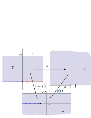
Figure 2. Composition of maps $f(z)=g(e^{z})$ for the proof of Lemma 2.4.

We investigate the conformal mapping $f|\Sigma$ in more detail. The preimage of $[-2,\infty)$ under $f|\Sigma$ is the curve $\gamma$ given by $\Re z=\log(\Im z/\sin\Im z)$, $0\leq\Im z<\pi$. This curve begins at the origin and becomes asymptotic to $\mathbb{R}+\pi i$ in the positive direction. By removing the curve $\gamma$, $\Sigma$ is cut into two parts, $\Sigma_{-}$ and $\Sigma_{+}$. $\Sigma_{-}$ is bounded by $\mathbb{R}^{-}$, $\gamma$ and $\mathbb{R}+\pi i$ with the latter line part of $\Sigma_{-}$. The region $\Sigma_{+}$ is bounded by $\gamma$ and $\mathbb{R}^{+}$. Then $f|\Sigma_{-}$ is a conformal mapping of $\Sigma_{-}$ onto the half-closed strip $S=\{w:0<\Im w\leq 2\pi\}$ with $f(\mathbb{R}+\pi i)=\mathbb{R}+2\pi i$, $f(\mathbb{R}^{-})=(-\infty,-2)$ and $f(\gamma)=[-2,+\infty)$. Similarly, $f|\Sigma_{+}$ is a conformal mapping of $\Sigma_{+}$ onto the lower half-plane $\overline{\mathbb{H}}=\{\bar{z}:z\in\mathbb{H}\}$, where $\bar{z}$ denotes the complex conjugate of $z$, with $f(\mathbb{R}^{+})=(-\infty,-2)$ and $f(\gamma)=[-2,+\infty)$. (See Fig 3.)

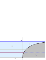
$\downarrow$f

Figure 3. Conformal maps $f|\Sigma_{-}$ and $f|\Sigma_{+}$.

Both maps $f|\Sigma_{-}$ and $f|\Sigma_{+}$ extend to conformal maps of larger regions. Because $f(\bar{z})=\overline{f(z)}$, $f$ maps $\overline{\Sigma_{+}}$ conformally onto $\mathbb{H}$. As $f(\mathbb{R}^{+})=(-\infty,-2)$, $f$ is a conformal map of $\Omega_{+}:=\Sigma_{+}\cup\mathbb{R}^{+}\cup\overline{\Sigma_{+}}$ onto the slit plane $\bar{\mathbb{H}}\cup(-\infty,-2)\cup\mathbb{H}=\mathbb{C}\setminus[-2,+\infty)$. Let $h_{+}:\mathbb{C}\setminus[-2,+\infty)\to\Omega_{+}$ be the inverse function for $f|\Omega_{+}$. The conformal extension of $f|\Sigma^{-}$ is more involved to describe. The fact that $f(\bar{z})=\overline{f(z)}$ implies $f$ maps $\overline{\Sigma_{-}}$ conformally onto $\bar{S}$. Since $f(\mathbb{R}^{-})=(-\infty,-2)$, $f$ is a conformal map of $\Delta_{0}=\Sigma_{-}\cup\mathbb{R}^{-}\cup\overline{\Sigma_{-}}$ onto the slit closed strip $S_{0}=S\cup(-\infty,-2)\cup\bar{S}=\{w:|\Im w|\leq 2\pi\}\setminus[-2,+\infty)$ with the upper (lower) edge of $\Delta_{0}$ corresponding to the upper (lower) edge of $S_{0}$. It is straightforward to verify that $f(z+2\pi i)=f(z)+4\pi i$ for each $n\in\mathbb{Z}$. This functional relationship implies that $f$ is a conformal map of $\Delta_{n}=\Delta_{0}+2\pi ni$ onto $S_{n}=S_{0}+4\pi ni$ for each $n\in\mathbb{Z}$. Hence, $f$ is a conformal map of $\Omega_{-}:=\cup_{n\in\mathbb{Z}}\Delta_{n}$ onto the infinitely slit plane $S_{\infty}:=\bigcup_{n\in\mathbb{Z}}S_{n}=\mathbb{C}\setminus\bigcup_{n\in\mathbb{Z}}\big{(}[-2,+\infty)+4\pi ni\big{)}$. Let $h_{-}:S_{\infty}\to\Omega_{-}$ be the inverse function of $f|\Omega_{-}$. Because $\mathbb{C}\setminus[-2,+\infty)\supset S_{\infty}$, we may regard $h_{+}$ as defined on $S_{\infty}$, so $h_{\pm}$ have a common domain. (See Fig. 4.)

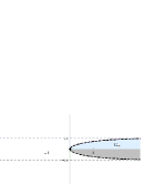
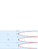
$\downarrow$${}^{f|\Omega_{+}}$	$\downarrow$${}^{f|\Omega_{-}}$

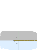
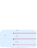
Figure 4. Conformal maps $f|\Omega_{+}$ and $f|\Omega_{-}$ with $\Omega_{+}:=\Sigma_{+}\cup\mathbb{R}^{+}\cup\overline{\Sigma_{+}}$ and $\Omega_{-}=\bigcup_{n=-\infty}^{\infty}\Delta_{n}$.

The two conformal maps $h_{\pm}$ just constructed provide analytic extensions to $S_{\infty}$ of the real-valued functions $h_{\pm}$. This allows us to define a pair of functions

(2.8) $$\varphi_{\pm}(z):=\frac{e^{k_{0}h_{\pm}(z)}}{(e^{h_{\pm}(z)}-1)^{2}}$$

which are analytic in $S_{\infty}$.

Lemma 2.5.

For each point $u\in(-\infty,-2)$ the power series expansion of $\varphi_{\pm}$ has radius of convergence $2-u$, $\varphi_{\pm}$ is analytic in the slit disk $D(u,r)\setminus[-2,+\infty)$, where $r=r(u)=\sqrt{(u+2)^{2}+16\pi^{2}}$. Furthermore, $\varphi_{\pm}(w)\approx-1/(w+2)$ as $w\to-2$ in $S_{\infty}$.

Proof.

For each point $u\in(-\infty,-2)$ the power series expansion of $h_{\pm}$ has radius of convergence $|u+2|$, the distance from $u$ to $-2$ because $-2$ is the closest singularity of $h_{\pm}$. Also, $h_{\pm}$ is analytic in the slit disk $D(u,r)\setminus[-2,+\infty)$, where $r=r(u)=\sqrt{(u+2)^{2}+16\pi^{2}}$ is the distance from $u$ to $-2\pm 4\pi i$.

Note that singularities of $\varphi_{-}$ that arise from $h_{-}(w)=2n\pi i$ are located at the slits taken out of $S_{\infty}$ and that $h_{+}(w)\in\Omega_{+}$ cannot take values in $2n\pi i$. Thus $\varphi_{\pm}$ is also analytic in the slit disk $D(u,r)\setminus[-2,+\infty)$.

Substituting $w=2(z-e^{z})$, we see that

$$\lim_{w\to-2,\;w\in S_{\infty}}(w+2)\varphi_{\pm}(w) = \lim_{w\to-2,\;w\in S_{\infty}}e^{k_{0}h_{\pm}(w)}\frac{w+2}{(e^{h_{\pm}(w)}-1)^{2}}$$

$$= 2\lim_{z\to 0,\;z\in\Omega_{\pm}}e^{k_{0}z}\frac{1+z-e^{z}}{(e^{z}-1)^{2}}\ =\ -1.$$

$\square$

Conclusion of proof of Proposition 2.1 for $\alpha=2$.

We now prove (1.11) and identify the limit. Using functions $\varphi_{\pm}$ constructed above, define

(2.9) $$\widetilde{G}(z,\lambda):=\begin{cases}(e^{\lambda}-1)^{2}\varphi_{+}(z(e^{\lambda}-1)^{2}+2\lambda-2e^{\lambda})&\mbox{ if $\lambda>0$ }\\ (e^{\lambda}-1)^{2}\varphi_{-}(z(e^{\lambda}-1)^{2}+2\lambda-2e^{\lambda})&\mbox{ if $\lambda<0$ }.\end{cases}$$

From Lemma 2.2 we see that function $\widetilde{G}(z,\lambda)$ satisfies (1.8) for all $(z,\lambda)\in\mathcal{D}_{+}\cup\mathcal{D}_{-}$. By uniqueness of the PDE solution in each of the two regions, $G(z,\lambda)=\widetilde{G}(z,\lambda)$ for all $(z,\lambda)\in\mathcal{D}_{+}\cup\mathcal{D}_{-}$. In particular, for each fixed $\lambda\neq 0$, $\limsup_{n\to\infty}(m_{n}(\lambda))^{1/n}$ is the reciprocal of the radius of convergence of the series expansion of $\widetilde{G}(z,\lambda)$ at $z=0$. The latter is $(1-e^{\lambda})^{-2}$ times the radius of convergence for $\varphi_{sign(\lambda)}(w)$ at $u=2\lambda-2e^{\lambda}\in(-\infty,-2)$ which by Lemma 2.5 is $2(e^{\lambda}-\lambda-1)$. Furthermore, the lemma implies that there is $\eta=\eta(\lambda)>0$ such that $\varphi_{sign(\lambda)}(w)$ is analytic on the slit disk $\{w:|w-u|<2(e^{\lambda}-\lambda-1)(1+\eta)\}\setminus[-2,\infty)$. Since after appropriate translation and re-scaling this slit disk is larger than the indented disk $\Delta(\pi/4,\eta)$ introduced in [25, (2.5)], and the second part of Lemma 2.5 gives $\varphi_{\pm}(w)\approx-1/(w+2)$ as $w\to-2$, we can apply [25, Corollary 2] to get (1.11).

Finally, as $m_{n}(0)=1$ the convergence at $\lambda=0$ holds trivially. $\square$

3. Proof of Theorem 1.3

We follow the method and notation of Dupuis-Ellis [20]. Although some arguments are analogous to those found in [20, Chapter 6] which considers random walk models with time-homogeneous continuous statistics, and [44] where a different model with a time singularity at $t=0$ is examined, for completeness we give all relevant details as several differ, especially in the lower bound proof.

Let $X^{n}_{j}=Z_{j-k_{0}+1}/n$ for $k_{0}\leq j\leq n$, and set $X^{n}_{j}=j/n$ for $0\leq j\leq k_{0}$. Then, noting (1.1), given $X^{n}_{j}$, we have $X^{n}_{j+1}=X^{n}_{j}+v^{n}_{j}/n$ where $v^{n}_{j}$ has Bernoulli distribution $\rho_{\sigma_{n}(j/n),X^{n}_{j}}$. Here,

$$\sigma_{n}(t) = \begin{cases}s_{\lfloor nt-k_{0}+1\rfloor}/n&\ {\rm for\ }t\geq\frac{k_{0}}{n}\\ 0&\ {\rm for\ }t<\frac{k_{0}}{n}\end{cases}$$

$$\rho_{\sigma,x}(A) = \frac{x}{\sigma}\delta_{0}(A)+\left(1-\frac{x}{\sigma}\right)\delta_{1}(A)\ \ \ \ \ {\rm for\ }A\subset\mathbb{R},\ 0\leq x\leq\sigma,$$

and $\rho_{0,0}:=\delta_{1}$.

Define $X^{n}_{\cdot}$ as the polygonal interpolated path connecting points $(j/n,X^{n}_{j})$ for $0\leq j\leq n$. Also, for probability measures $\mu\ll\nu$ such that $d\mu=fd\nu$, denote $R(\mu\|\nu)=\int f\log fd\nu$, the relative entropy; set $R(\mu\|\nu)=\infty$ when $\mu$ is not absolutely continuous with respect to $\nu$.

Let $h:C([0,1],\mathbb{R})\rightarrow\mathbb{R}$ be a bounded continuous function. To prove Theorem 1.3, we need only establish Laplace principle upper and lower bounds [20, page 74]. The upper bounds are to show

$$\limsup_{n\rightarrow\infty}\frac{1}{n}\log E\big{\{}\exp[-nh(X^{n}_{\cdot})]\big{\}}\ \leq\ -\inf_{\varphi\in\mathcal{C}_{1}}\big{\{}I(\varphi)+h(\varphi)\big{\}}$$

for a rate function $I$ and a closed subset of continuous functions $\mathcal{C}_{1}$. The lower bounds are to prove the reverse inequality

$$\liminf_{n\rightarrow\infty}\frac{1}{n}\log E\big{\{}\exp[-nh(X^{n}_{\cdot})]\big{\}}\ \geq\ -\inf_{\varphi\in\mathcal{C}_{1}}\big{\{}I(\varphi)+h(\varphi)\big{\}}.$$

Define, for $k_{0}+1\leq j\leq n$, noting $X^{n}_{j}=j/n$ for $j\leq k_{0}$ is deterministic, that

$$W^{n}(j,x_{j},\ldots,x_{k_{0}+1})\ =\ -\frac{1}{n}\log E\Big{[}e^{-nh(X^{n}_{\cdot})}\Big{|}X^{n}_{j}=x_{j},\ldots,X^{n}_{k_{0}+1}=x_{k_{0}+1}\Big{]},$$

and

$$W^{n}\ :=\ W^{n}(k_{0},\emptyset)\ =\ -\frac{1}{n}\log E\Big{[}e^{-nh(X^{n}_{\cdot})}\Big{]}.$$

Then, by the Markov property, for $k_{0}+1\leq j\leq n-1$,

$$e^{-nW^{n}(j,x_{j},\ldots,x_{k_{0}+1})} = E\Big{[}e^{-nW^{n}(j+1,X^{n}_{j+1},x_{j},\ldots,x_{k_{0}+1})}\Big{|}X^{n}_{j}=x_{j},\ldots,X^{n}_{k_{0}+1}=x_{k_{0}+1}\Big{]}$$

$$= \int e^{-nW^{n}(j+1,x_{j}+v/n,x_{j},\ldots,x_{k_{0}+1})}d\rho_{\sigma_{n}(j/n),x_{j}}(dv).$$

By a property of relative entropy [20, Prop. 1.4.2 (a)], for $k_{0}+1\leq j\leq n-1$,

$$W^{n}(j,x_{j},\ldots,x_{k_{0}+1})$$

$$=\ -\frac{1}{n}\log\int e^{-nW^{n}(j+1,x_{j}+y/n,x_{j},\ldots,x_{k_{0}+1})}\rho_{\sigma_{n}(j/n),x_{j}}(dv)$$

$$=\ \inf_{\gamma}\Big{\{}\frac{1}{n}R(\gamma\|\rho_{\sigma_{n}(j/n),x_{j}})+\int W^{n}(j+1,x_{j}+y/n,x_{j},\ldots,x_{1})\gamma(dy)\Big{\}}.$$

Also, the boundary condition $W^{n}(n,x_{n},\ldots,x_{k_{0}+1})=h(x_{\cdot})$ holds with respect to the linearly interpolated path $x_{\cdot}=x^{n}_{\cdot}$ connecting $\{(l/n,l/n)\}_{0\leq l\leq k_{0}}$,

The basic observation in the Dupuis-Ellis method is that $W^{n}(j,x_{j},\ldots,x_{k_{0}+1})$ satisfies a control problem ([20, section 3.2]) whose solution for $k_{0}\leq j\leq n-1$ is

$$V^{n}(j,x_{j},\ldots,x_{k_{0}+1})\ =\ \inf_{\{v^{n}_{i}\}}\bar{E}_{j,x_{j},\ldots,x_{k_{0}+1}}\Big{\{}\frac{1}{n}\sum_{i=j}^{n-1}R(v^{n}_{i}(\cdot)\|\rho_{\sigma_{n}(i/n),\bar{X}^{n}_{i}})+h(\bar{X}^{n}_{\cdot})\Big{\}}.$$

Here, $v^{n}_{i}(dy)=v^{n}_{i}(dy;x_{k_{0}},\ldots,x_{i})$ is a Bernoulli distribution given $x_{k_{0}},\ldots,x_{i}$ for $k_{0}\leq i\leq n-1$ and in the display $\nu^{n}_{i}(\cdot)=\nu^{n}_{i}(dy|\bar{X}^{n}_{k_{0}},\ldots,\bar{X}^{n}_{i})$; $\{\bar{X}^{n}_{i};0\leq i\leq n\}$ is the adapted path satisfying $\bar{X}^{n}_{l}=l/n$ for $0\leq l\leq k_{0}$, and $\bar{X}^{n}_{l+1}=\bar{X}^{n}_{l}+\bar{Y}^{n}_{l}/n$ for $k_{0}\leq l\leq n-1$ where $\bar{Y}^{n}_{l}$, conditional on $(\bar{X}^{n}_{l},\ldots\bar{X}^{n}_{k_{0}})$ has distribution $v^{n}_{l}(\cdot)$; $\bar{X}^{n}_{\cdot}$ is the interpolated path with respect to $\{\bar{X}^{n}_{l}\}$; and $\bar{E}_{j,x_{j},\ldots,x_{k_{0}+1}}$ denotes conditional expectation with respect to the $\bar{X}^{n}_{\cdot}$ process given the values $\{\bar{X}^{n}_{l}=x_{l}:k_{0}+1\leq l\leq j\}$ at step $k_{0}+1\leq j\leq n$. The boundary conditions are $V^{n}(n,x_{n},\ldots,x_{k_{0}+1})=h(x_{\cdot})$ and

(3.1) $$V^{n}(k_{0},\emptyset)=V^{n}=\inf_{\{v^{n}_{j}\}}\bar{E}\Big{\{}\frac{1}{n}\sum_{j=k_{0}}^{n-1}R(v^{n}_{j}(\cdot)\|\rho_{\sigma_{n}(j/n),\bar{X}^{n}_{j}})+h(\bar{X}^{n}_{\cdot})\Big{\}}.$$

In particular, by [20, Corollary 5.2.1],

(3.2) $$W^{n}\ =\ -\frac{1}{n}\log E\Big{[}e^{-nh(X^{n}_{\cdot})}\Big{]}\ =\ V^{n}.$$

The goal will be to take Laplace limits using this representation. To simply later expressions, we will take $v^{n}_{j}=\delta_{1}$ for $0\leq j\leq k_{0}-1$ when $k_{0}\geq 1$.

3.1. Upper bound

To establish the upper bound, we first put the controls $\{v^{n}_{j}\}$ into continuous time paths: Let $v^{n}(dy|t)=v^{n}_{j}(dy)$ for $t\in(j/n,(j+1)/n],\;0\leq j\leq n-1$, and $v^{n}(dy|0)=v^{n}_{0}$. Define

$$v^{n}(A\times B)\ =\ \int_{B}v^{n}(A|t)dt$$

for $A\subset\mathbb{R}$, $B\subset[0,1]$. Define also the piecewise constant path $\tilde{X}^{n}(t)=\bar{X}^{n}_{j}$ for $t\in(j/n,(j+1)/n],\;0\leq j\leq n-1$, and $\tilde{X}^{n}(0)=0$. Then,

(3.3) $$V^{n} = \inf_{\{v^{n}_{j}\}}\bar{E}\Big{\{}\int_{0}^{1}R(v^{n}(\cdot|t)\|\rho_{\sigma_{n}(\lfloor nt\rfloor/n),\tilde{X}^{n}(t)})dt+h(\bar{X}^{n}_{\cdot})\Big{\}}.$$

From this control representation, as $|V^{n}|=|W^{n}|\leq\|h\|_{\infty}$ and $\rho_{\sigma,x}$ is supported on $K=\{0,1\}$, for each $n$, there is $\{v^{n}_{j}\}$ supported on $K$ and corresponding $v^{n}(dy\times dt)=v^{n}(dy|t)\times dt$ such that

$$W^{n}+\epsilon\ =\ V^{n}+\epsilon\ \geq\ \bar{E}\Big{[}\int_{0}^{1}R(v^{n}(\cdot|t)\|\rho_{\sigma_{n}(\lfloor nt\rfloor/n),\tilde{X}^{n}(t)})dt+h(\bar{X}^{n}_{\cdot})\Big{]}.$$

As the sets $K$ and

$$\Gamma\ =\ \Big{\{}\varphi\in C([0,1];\mathbb{R}):\;\varphi(0)=0,\;\varphi\uparrow,\ {\rm Lipschitz,\ with\ bound\ }1\Big{\}}$$

are compact on $\mathbb{R}$ and $C([0,1],\mathbb{R})$ respectively, and $\{v^{n}_{j}\}$ are probability measures on $K$ and $\{\bar{X}^{n}_{\cdot}\}\subset\Gamma$, by Prokhorov’s theorem, the distributions of $(v^{n}(dy\times dt),\bar{X}^{n}_{\cdot})$ have a subsequence which converges weakly to a limit distribution governing $(v,\bar{X}_{\cdot})$ where for each realization, $v$ is a probability measure on $K\times[0,1]$ and $\bar{X}_{\cdot}\in\Gamma$. More precisely, let $(\bar{\Omega},\bar{F},\bar{P})$ be a probability space where $v:\bar{\Omega}\rightarrow{\rm probability\ measures\ on\ }K\times[0,1]$, and $\bar{X}:\bar{\Omega}\rightarrow\Gamma$. Then, [20, Lemma 3.3.1] gives that $v$ is the subsequential weak limit of $v^{n}$, and $\bar{P}$-a.s. for $\omega\in\bar{\Omega}$,

$$v(A\times B|\omega)\ =\ \int_{B}v(A|t,\omega)dt$$

for some kernel $v(dy|t,\omega)$ on $K$ given $t$ and $\omega$.

Now, by the same proof given for [20, Theorem 5.3.5] (only [20, equation (5.12)] in the theorem statement differs; in our context $\mu$ there is replaced by $\rho_{\sigma_{n}(j/n),\tilde{X}^{n}_{j}}$), as $K$ is compact, we have $(v^{n},\bar{X}^{n},\tilde{X}^{n})$ has a subsequential limit in distribution to $(v,\bar{X},\bar{X})$ [the last coordinate with respect to $D([0,1],\mathbb{R})$]. Also, $\bar{P}$-a.s., for all $t\in[0,1]$,

$$\bar{X}(t)\ =\ \int_{\mathbb{R}\times[0,1]}yv(dy\times ds)\ =\ \int_{0}^{t}\int_{K}yv(dy|s)ds.$$

In particular, $\bar{P}$-a.s., $\dot{\bar{X}}(t)=\int_{K}yv(dy|t)$.

By Skorohod representation theorem, we can assume $(v^{n},\bar{X}^{n},\tilde{X}^{n})\rightarrow(v,\bar{X},\bar{X})$ converges a.s. In particular, $\bar{X}^{n}$ converges uniformly to $\bar{X}$ a.s., and it is clear that $\tilde{X}^{n}$ converges uniformly to $\bar{X}$ a.s. as $\bar{X}$ is continuous ([20, p. 154]).

Let $\mu_{\delta}(\cdot)=(1-\delta)^{-1}1_{[\delta,1]}(\cdot)$ and $\nu^{n}(dy\times\mu_{\delta}dt)=\nu^{n}(dy|t)\times\mu_{\delta}dt$. Then, by [20, Lemma 1.4.3 (f)] we have, for $0<\delta<1$, that

$$\int_{\delta}^{1}R\big{(}v^{n}(\cdot|t)\big{\|}\rho_{\sigma_{n}(\lfloor nt\rfloor/n),\tilde{X}^{n}(t)}\big{)}dt$$

$$\ \ \ \ \ \ \ \ \ =\ (1-\delta)R\big{(}v^{n}(dy\times\mu_{\delta}dt)\Big{\|}\rho_{\sigma_{n}(\lfloor nt\rfloor/n),\tilde{X}^{n}(t)}\times\mu_{\delta}dt\big{)}.$$

Write,

$$\liminf_{n\to\infty}V^{n} \geq \liminf_{n\rightarrow\infty}\bar{E}\Big{[}\int_{\delta}^{1}R\big{(}v^{n}(\cdot|t)\big{\|}\rho_{\sigma_{n}(\lfloor nt\rfloor/n),\tilde{X}^{n}(t)}\big{)}dt+h(\bar{X}^{n}_{\cdot})\Big{]}$$

$$\geq \liminf_{n\rightarrow\infty}\bar{E}\Big{[}(1-\delta)R\Big{(}v^{n}(dy\times\mu_{\delta}dt)\Big{\|}\rho_{\sigma_{n}(\lfloor nt\rfloor/{n}),\tilde{X}^{n}(t)}\times\mu_{\delta}dt\Big{)}+h(\bar{X}_{\cdot})\Big{]}$$

$$\geq \bar{E}\Big{[}\int_{\delta}^{1}R(v(\cdot|t)\|\rho_{\alpha t,\bar{X}(t)})dt+h(\bar{X}_{\cdot})\Big{]}$$

where in the last line we use Fatou’s lemma, noting lower semi-continuity of $R$, $\nu^{n}(dy\times\mu_{\delta}dt)\rightarrow\nu(dy|t)\times\mu_{\delta}dt$ a.s., and $\rho_{\sigma_{n}(\lfloor nt\rfloor/n),\tilde{X}^{n}(t)}$ converges in distribution to $\rho_{\alpha t,\bar{X}(t)}$ for $t\in[\delta,1]$ a.s. since $\sigma_{n}(\lfloor nt\rfloor/n)\rightarrow\alpha t$, $\tilde{X}^{n}(t)\rightarrow\bar{X}(t)$ uniformly on $[0,1]$ a.s., and $\rho_{\sigma,x}$ is continuous on $\{(\sigma,x):\delta\leq\sigma\leq 1,0\leq x\leq\sigma\}$ (cf. Section 6.2 [20]).

By [20, Lemma 3.3.3(b)],

$$R(v(\cdot|t)\|\rho_{\alpha t,\bar{X}(t)})\ \geq\ L\left(\alpha t,\bar{X}(t),\int yv(dy|t)\right)$$

where

(3.4) $$L(t,x,y) = \sup_{\theta}\Big{\{}\theta y-\log\int e^{\theta z}\rho_{t,x}(dz)\Big{\}}.$$

We note, for $t>0$, $L(t,x,y)$ diverges when $x=0$, $0\leq y<1$, and $x=t$, $0<y\leq 1$ but is finite when $0<x<t$ and $0\leq y\leq 1$, and in this case evaluates to

(3.5) $$L(t,x,y) = y\log\left(\frac{ty}{t-x}\right)+(1-y)\log\left(\frac{t(1-y)}{x}\right),$$

understood with the usual convention $0\log(0)=0$.

Since $\int yv(dy|t)=\dot{\bar{X}}(t)$, we have

$$\liminf_{n\to\infty}V^{n}\ \geq\ \bar{E}\Big{[}\int_{\delta}^{1}L(\alpha t,\bar{X}(t),\dot{\bar{X}}(t))dt+h(\bar{X}_{\cdot})\Big{]}.$$

As $L\geq 0$, and $\bar{X}(\cdot)\in\Gamma$, letting $\delta\downarrow 0$, we obtain,

$$\liminf_{n\to\infty}V^{n}\ \geq\ \inf_{\varphi\in\Gamma}\int_{0}^{1}L(\alpha t,\varphi(t),\dot{\varphi}(t))dt+h(\varphi).$$

Taking into account (3.2), the upper bound holds with $\mathcal{C}_{1}=\Gamma$ and

$$I(\varphi)\ =\ \int_{0}^{1}L(\alpha t,\varphi(t),\dot{\varphi}(t))\,dt.$$

3.2. Lower bound

In the following, for typographical convenience, we write $E(X;\mathbb{A})$ for $\int_{\mathbb{A}}XdP$. Let now $\psi^{*}\in\Gamma$ be such that $I(\psi^{*})<\infty$, and fix a bounded, continuous (in the sup norm) function $h:C([0,1];\mathbb{R})\to\mathbb{R}$. In view of (3.2), we need only show, for each $\varepsilon>0$, that

(3.6) $$\limsup_{n\to\infty}V^{n}\ \leq\ I(\psi^{*})+h(\psi^{*})+8\varepsilon.$$

Step 1. Our first goal is to replace $\psi^{*}$ by its appropriate regularization. We use the trick of considering a convex combination of paths,

$$\psi_{\theta}(t)\ =\ (1-\theta)\psi^{*}(t)+\theta t$$

for $0\leq\theta\leq 1$. Since $\|\psi_{\theta}-\psi^{*}\|_{\infty}\leq 2\theta$, it is clear, for small enough $\theta>0$, that $|h(\psi_{\theta})-h(\psi^{*})|<\varepsilon$. Further, since $I$ is finite on the line $y=t$ with slope $1$, by convexity arguments [20, Lemma 1.4.3 (b)], for small enough $\theta>0$,

$$I(\psi_{\theta})\ \leq\ I(\psi^{*})+\varepsilon.$$

We therefore fix $\theta>0$ such that $I(\psi_{\theta})<I(\psi^{*})+\varepsilon$ and $h(\psi_{\theta})<h(\psi^{*})+\varepsilon$.

Next, following [20, p. 82], we write

(3.7) $$\varphi_{\kappa}(t)\ =\ \int_{0}^{t}\gamma_{\kappa}(s)ds,$$

where

$$\gamma_{\kappa}(t)\ =\ \kappa\int_{i/\kappa}^{i+1/\kappa}\dot{\psi_{\theta}}(s)ds$$

for $t\in(i/\kappa,(i+1)/\kappa]$, $0\leq i\leq\kappa-1$, and $\gamma_{\kappa}(0)=\gamma_{\kappa}(1/\kappa)$. For large enough $\kappa$, we have

(3.8) $$\frac{\varphi_{\kappa}(t)}{t} \geq \theta\ >\ 0$$

(3.9) $$h(\varphi_{\kappa}) \leq h(\psi^{*})+2\varepsilon$$

(3.10) $$I(\varphi_{\kappa}) \leq I(\psi^{*})+2\varepsilon.$$

Inequality (3.8) is a property of $\psi_{\theta}$, and is preserved by (3.7). Since

$$\lim_{\kappa\rightarrow\infty}\sup_{t\in[0,1]}|\psi_{\theta}(t)-\varphi_{\kappa}(t)|\ =\ 0,$$

inequality (3.9) follows from continuity of $h$ by our choice of $\theta$. Then, as

$$\dot{\varphi}_{\kappa}(t)\ =\ \kappa\int_{\lfloor t\kappa\rfloor/\kappa}^{\lceil t\kappa\rceil/\kappa}\dot{\psi_{\theta}}(s)ds\ \rightarrow\ \dot{\psi_{\theta}}(t)$$

as $\kappa\uparrow\infty$, and $(t,x,y)\mapsto L(\alpha t,x,y)$ (cf. (3.4),(3.5)) as $\alpha>1$ is bounded, uniformly continuous on the compact set

$$\Big{\{}(t,x,y):\;0\leq t\leq 1,\;\theta t\leq x\leq t,\;\theta\leq y\leq 1\Big{\}},$$

by the dominated convergence theorem, $\lim_{\kappa}I(\varphi_{\kappa})=I(\psi_{\theta})$. Inequality (3.10) follows due to our choice of $\theta$.

We now fix $\kappa$ such that the above bounds hold.

Since (3.10) implies $I(\varphi_{\kappa})<\infty$, we now choose a $0<\delta<1/3$ such that

(3.11) $$\int_{0}^{\delta}L(\alpha t,\varphi_{\kappa}(t),\dot{\varphi}_{\kappa}(t))dt\ <\ \varepsilon.$$

We will also need an estimate on $s_{n}$. From assumptions (1.2), there is an $0<\eta<1/2$ and $k_{1}\geq k_{0}+1$ such that for $n\geq k_{1}$,

(3.12) $$\eta\ \leq\ \frac{n}{s_{n-k_{0}+1}}\ \leq\ 1-\eta.$$

With respect to $\eta$ and $\theta$, we impose additionally that $\delta$ satisfies

(3.13) $$-\delta\log(\delta\eta\theta)\ <\ \varepsilon/10.$$

Step 2. We now build a sequence of controls based on $\varphi_{\kappa}$. Recall that we already set $v^{n}_{j}(dy)=\delta_{1}$ for $0\leq j\leq k_{0}-1$ when $k_{0}\geq 1$. Define

$$v^{n}_{j}(dy;x_{k_{0}},\dots,x_{j})\ =\ \begin{cases}\rho_{\sigma_{n}(j/n),{x}_{j}}&\ {\rm for\ }k_{0}\leq j\leq k_{1}\\ \rho_{1,1-\dot{\varphi}_{\kappa}(j/n)}&\ {\rm for\ }j\geq k_{1}+1.\end{cases}$$

Note, for $j\geq k_{1}+1$, $\nu^{n}_{j}$ does not depend on auxiliary inputs $x_{k_{0}},\ldots,x_{j}$, and is in fact the Bernoulli distribution with success probability $\dot{\varphi}_{\kappa}(j/n)$.

Define also $\bar{X}^{n}_{l}=l/n$ for $0\leq l\leq k_{0}$, and $\bar{X}^{n}_{j+1}=\bar{X}^{n}_{j}+\bar{Y}^{n}_{j}/n$ for $j\geq k_{0}$ where

$$\bar{P}(\bar{Y}^{n}_{j}\in dy|\bar{X}^{n}_{0},\ldots,\bar{X}^{n}_{j})\ =\ v_{j}(dy;\bar{X}^{n}_{0},\ldots,\bar{X}^{n}_{j}).$$

Thus, for $j\geq 1$, $\bar{X}^{n}_{j}=(1/n)\sum_{\ell=0}^{j-1}Y^{n}_{\ell}$ where $\{Y^{n}_{j}\}_{j\geq k_{1}+1}$ are independent Bernoulli random variables with corresponding means $\{\dot{\varphi}_{\kappa}(j/n)\}_{j\geq k_{1}+1}$.

Step 3. We now collect some useful estimates.A. Since $\bar{Y}^{n}_{0}\equiv 1$ (when $k_{0}=0$, recall $\rho_{\sigma,0}=\delta_{1}$), and the increments are at most one, we have $1/n\leq\bar{X}^{n}_{j}\leq j/n$ for $1\leq j\leq n$.

B. We have

(3.14) $$\lim_{n\uparrow\infty}\sup_{0\leq j/n\leq 1}\left|\bar{X}^{n}_{j}-\frac{1}{n}\sum_{l=0}^{j}\dot{\varphi}_{\kappa}(l/n)\right|\ =\ 0\ \ \ \ \ {\rm a.s.}$$

Indeed, for large enough $n$, as $0\leq\dot{\varphi}_{\kappa}\leq 1$, $(1/n)\sum_{j=0}^{k_{1}}|\dot{\varphi}_{\kappa}(j/n)|+k_{1}/n<n^{-1/8}$. Then, by Doob’s maximal inequality,

$$\bar{P}\Big{[}\sup_{0\leq j/n\leq 1}\Big{|}\bar{X}^{n}_{j}-\frac{1}{n}\sum_{l=0}^{j}\dot{\varphi}_{\kappa}(l/n)\Big{|}>\frac{\theta}{2n^{1/8}}\Big{]}$$

$$\ \ \ \ \leq\ Cn^{1/2}\bar{E}\Big{|}\bar{X}^{n}_{n}-\bar{E}(X_{n}^{n})\Big{|}^{4}$$

$$\ \ \ \ \leq\ \frac{1}{n^{7/2}}\Big{[}C\sum_{l=0}^{n}\dot{\varphi}_{\kappa}(l/n)(1-\dot{\varphi}_{\kappa}(l/n))(1-3\dot{\varphi}_{\kappa}(l/n)+3\dot{\varphi}_{\kappa}^{2}(l/n))$$

(3.15) $$\ \ \ \ \ \ \ \ \ \ \ \ \ \ \ \ \ +\ C\left(\sum_{l=0}^{n}\dot{\varphi}_{\kappa}(l/n)(1-\dot{\varphi}_{\kappa}(l/n))\right)^{2}\Big{]}\ \leq\ {C}n^{-3/2}.$$

where $C$ is a constant changing line to line.

C. For $0\leq j\leq n$, from (3.8), it follows that

(3.16) $$\frac{1}{n}\sum_{l=0}^{j}\dot{\varphi}_{\kappa}(l/n)\ \geq\ \theta\frac{j}{n}.$$

D. Let $j\geq k_{1}+1$. Noting $1/n\leq\bar{X}^{n}_{j}\leq j/n$ (cf. part A) and bounds (3.12), we have

$$\eta\leq 1-\frac{j}{s_{j-k_{0}+1}}\leq 1-\frac{\bar{X}^{n}_{j}}{\sigma_{n}(j/n)}\leq 1,\ \ \ \frac{1}{s_{j-k_{0}+1}}\leq\frac{\bar{X}^{n}_{j}}{\sigma_{n}(j/n)}\leq 1-\eta.$$

Hence, $L(\sigma_{n}(j/n),\bar{X}^{n}_{j},\dot{\varphi}_{\kappa}(j/n))$ can be well evaluated (cf. (3.4), (3.5)), and we may rewrite the relative entropy as

$$R(v^{n}_{j}\|\rho_{\sigma_{n}(j/n),\bar{X}^{n}_{j}}) = \dot{\varphi}_{\kappa}(j/n)\log[\dot{\varphi}_{\kappa}(j/n)/(1-\bar{X}^{n}_{j}/\sigma_{n}(j/n))]$$

$$\ \ \ +(1-\dot{\varphi}_{\kappa}(j/n))\log\big{(}(1-\dot{\varphi}_{\kappa}(j/n))/(\bar{X}^{n}_{j}/\sigma_{n}(j/n))\big{)}$$

$$= L(\sigma_{n}(j/n),\bar{X}^{n}_{j},\dot{\varphi}_{\kappa}(j/n)).$$

Further, as $0\leq\dot{\varphi}_{\kappa}\leq 1$, we have

$$L(\sigma_{n}(j/n),\bar{X}^{n}_{j},\dot{\varphi}_{\kappa}(j/n))$$

$$\ \ \ \ \ =\ \big{[}\dot{\varphi}_{\kappa}(j/n)\log\dot{\varphi}_{\kappa}(j/n)+(1-\dot{\varphi}_{\kappa}(j/n))\log(1-\dot{\varphi}_{\kappa}(j/n))\big{]}$$

$$\ \ \ \ \ \ \ \ \ \ \ \ \ -\dot{\varphi}_{\kappa}(j/n)\log\big{(}1-{\bar{X}_{j}^{n}}/{\sigma_{n}(j/n)}\big{)}-(1-\dot{\varphi}_{\kappa}(j/n))\log\big{(}{\bar{X}_{j}^{n}}/{\sigma_{n}(j/n)}\big{)}$$

(3.17) $$\ \ \ \ \ \leq\ 0-\log\eta+\log(s_{j-k_{0}+1})\ \leq\ \log(j/\eta^{2}),$$

the last inequality using (3.12) again.

Step 4. We now argue (3.6) via representation (3.1). Let

$$\mathbb{A}\ =\ \Big{\{}\sup_{0\leq j\leq n-1}|\bar{X}^{n}_{j}-\frac{1}{n}\sum_{l=0}^{j}\dot{\varphi}_{\kappa}(l/n)|>\frac{\theta}{2n^{1/8}}\Big{\}}.$$

Since $R(v^{n}_{j}\|\rho_{\sigma_{n}(j/n),\bar{X}^{n}_{j}})=0$ for $k_{0}\leq j\leq k_{1}$, the sum in (3.1) equals

(3.18) $$\bar{E}\Big{[}\frac{1}{n}\sum_{j=k_{0}}^{n-1}R(v^{n}_{j}\|\rho_{\sigma_{n}(j/n),\bar{X}^{n}_{j}})\Big{]} = \bar{E}\Big{[}\frac{1}{n}\sum_{j=k_{1}+1}^{n-1}L(\sigma_{n}(j/n),\bar{X}^{n}_{j},\dot{\varphi}_{\kappa}(j/n))\Big{]}$$

$$= \bar{E}\Big{[}\frac{1}{n}\sum^{n-1}_{j=k_{1}+1}L(\sigma_{n}(j/n),\bar{X}_{j}^{n},\dot{\varphi}_{\kappa}(j/n));\mathbb{A}\Big{]}$$

$$\ \ +\ \bar{E}\Big{[}\frac{1}{n}\sum_{j=k_{1}+1}^{n-1}L(\sigma_{n}(j/n),\bar{X}_{j}^{n},\dot{\varphi}_{\kappa}(j/n));\mathbb{A}^{c}\Big{]}$$

$$= A_{1}+A_{2}.$$

Step 5. We now treat the first term $A_{1}$ in (3.18). Combining (3.17) with (3.15), we obtain, for large $n$,

$$\bar{E}\Big{[}\frac{1}{n}\sum^{n-1}_{j=k_{1}+1}L(\sigma_{n}(j/n),\bar{X}_{j}^{n},\dot{\varphi}_{\kappa}(j/n));{\sup_{0\leq j\leq n-1}|\bar{X}^{n}_{j}-\frac{1}{n}\sum_{l=0}^{j}\dot{\varphi}_{\kappa}(l/n)|>\frac{\theta}{2n^{1/8}}}\Big{]}$$

$$\ \leq\ \log(n/\eta^{2})\bar{P}\Big{[}\sup_{0\leq j/n\leq 1}\Big{|}\bar{X}^{n}_{j}-\frac{1}{n}\sum_{l=0}^{j}\dot{\varphi}_{\kappa}(l/n)\Big{|}>\frac{\theta}{2n^{1/8}}\Big{]}$$

(3.19) $$\ \leq\ C\log(n/\eta^{2})n^{-3/2}\ <\ \varepsilon.$$

Step 6. For the other term $A_{2}$ in (3.18), we split it into two sums depending on when index $j\leq\delta n$ or $j\geq\delta n$ (recall $\delta$ from (3.11)):

$$\bar{E}\Big{[}\frac{1}{n}\sum_{j=k_{1}+1}^{\lfloor\delta n\rfloor}L(\sigma_{n}(j/n),\bar{X}_{j}^{n},\dot{\varphi}_{\kappa}(j/n));\mathbb{A}^{c}\Big{]}$$

$$\ \ \ \ \ \ \ \ \ \ \ \ \ \ +\ \bar{E}\Big{[}\frac{1}{n}\sum_{j=\lceil\delta n\rceil}^{n-1}L(\sigma_{n}(j/n),\bar{X}_{j}^{n},\dot{\varphi}_{\kappa}(j/n));\mathbb{A}^{c}\Big{]}$$

(3.20) $$=\ B_{1}+B_{2}.$$

Step 7. To estimate $B_{1}$, we divide it further into two terms corresponding to sums on indices $j\leq n^{7/8}$ and $n^{7/8}\leq j\leq\delta n$:

$$\bar{E}\Big{[}\frac{1}{n}\sum^{\lfloor n^{7/8}\rfloor}_{j=k_{1}+1}L(\sigma_{n}(j/n),\bar{X}_{j}^{n},\dot{\varphi}_{\kappa}(j/n));\mathbb{A}^{c}\Big{]}$$

$$\ \ \ \ \ \ \ \ \ \ \ \ \ \ +\ \bar{E}\Big{[}\frac{1}{n}\sum^{\lfloor\delta n\rfloor}_{j=\lceil n^{7/8}\rceil}L(\sigma_{n}(j/n),\bar{X}_{j}^{n},\dot{\varphi}_{\kappa}(j/n));\mathbb{A}^{c}\Big{]}$$

$$\ \ =\ D_{1}+D_{2}.$$

The first term $D_{1}$, using (3.17), is bounded for all large $n$ by

(3.21) $$n^{-1/8}\log(n^{7/8}/\eta^{2})\ <\ \varepsilon.$$

The second term $D_{2}$, using again (3.17), is bounded in absolute value by

$$-\delta\log\eta+\frac{1}{n}\sum_{j=\lceil n^{7/8}\rceil}^{\lfloor\delta n\rfloor}|\log(s_{j-k_{0}+1}/n)|$$

$$\ \ -\bar{E}\Big{[}\frac{1}{n}\sum_{j=\lceil n^{7/8}\rceil}^{\lfloor\delta n\rfloor}\log\bar{X}_{j}^{n};\sup_{0\leq j\leq n-1}|\bar{X}_{j}^{n}-\frac{1}{n}\sum_{l=0}^{j}\dot{\varphi}_{\kappa}(l/n)|\leq\frac{\theta}{2n^{1/8}}\Big{]}.$$

Now, note that (3.12) implies for $j\geq k_{1}+1$ that

$$\frac{j}{(1-\eta)n}\ \leq\ \frac{s_{j-k_{0}+1}}{n}\ \leq\ \frac{j}{\eta n}.$$

Then, as $0<\delta<1/3$ and $0<\eta<1/2$, we have for large $n$ that

$$\frac{1}{n}\sum_{j=\lceil n^{7/8}\rceil}^{\lfloor\delta n\rfloor}|\log(s_{j-k_{0}+1}/n)| \leq 2\int_{0}^{\delta}\max\Big{\{}\Big{|}\log\Big{(}\frac{x}{1-\eta}\Big{)}\Big{|},\Big{|}\log\Big{(}\frac{x}{\eta}\Big{)}\Big{|}\Big{\}}\,dx$$

$$\leq -6\delta\log\delta-2\delta\log\eta.$$

Also, noting (3.16), we have for large $n$ that

$$-\bar{E}\Big{[}\frac{1}{n}\sum_{j=\lceil n^{7/8}\rceil}^{\lfloor\delta n\rfloor}\log\bar{X}_{j}^{n};\sup_{0\leq j\leq n-1}|\bar{X}_{j}^{n}-\frac{1}{n}\sum_{l=0}^{j}\dot{\varphi}_{\kappa}(l/n)|\leq\frac{\theta}{2n^{1/8}}\Big{]}$$

$$\ \ \leq\ -\frac{1}{n}\sum_{j=\lceil n^{7/8}\rceil}^{\lfloor\delta n\rfloor}\log\Big{[}\frac{\theta j}{n}-\frac{\theta}{2n^{1/8}}\Big{]}$$

$$\ \ \leq\ -\frac{1}{n}\sum_{j=\lceil n^{7/8}\rceil}^{\lfloor\delta n\rfloor}\log\Big{[}\frac{\theta j}{2n}\Big{]}\ \leq\ -2\int_{0}^{\delta}\log\frac{\theta x}{2}\,dx\ \leq\ -4\delta\log\delta-2\delta\log\theta.$$

By combining these estimates, we have $D_{2}$ is bounded by a function of $\delta,\eta,\theta$ which, given (3.13), can be made small:

(3.22) $$D_{2}\ \leq\ -10\delta\log\delta-3\delta\log\eta-2\delta\log\theta\ <\ \varepsilon.$$

Step 8. We now estimate the second term $B_{2}$ in (3.20). Note, for $n>\delta^{-8}$, by (3.16) the event

$$\Big{\{}\sup_{0\leq j\leq n-1}|\bar{X}^{n}_{j}-\frac{1}{n}\sum_{l=0}^{j}\dot{\varphi}_{\kappa}(l/n)|\leq\frac{\theta}{2n^{1/8}}\Big{\}}\\ \ \subset\ \Big{\{}\inf_{j\geq\delta n}\bar{X}^{n}_{j}\geq\frac{\delta\theta}{2}\Big{\}}.$$

Hence, for large $n$,

$$B_{2} \leq \bar{E}\Big{[}\frac{1}{n}\sum_{j=\lceil\delta n\rceil}^{n-1}L(\sigma_{n}(j/n),\bar{X}^{n}_{j},\dot{\varphi}_{\kappa}(j/n));\mathbb{A}^{c}\cap\Big{\{}\inf_{j\geq\delta n}\bar{X}^{n}_{j}\geq\frac{\delta\theta}{2}\Big{\}}\Big{]}.$$

Note, from assumption (1.2) and $\bar{X}^{n}_{j}\leq j/n$, that $\delta/(1-\eta)\leq\sigma_{n}(j/n)\leq 1/\eta$ and $\bar{X}^{n}_{j}\leq\sigma_{n}(j/n)(1-\eta)$ when $\delta\leq j/n\leq 1$ for all large $n$. Also, $L(t,x,y)$ is continuous, and therefore also bounded and uniformly continuous on the compact set (cf. definition of $L$ (3.4), (3.5)),

(3.23) $$\Big{\{}(t,x,y):\;\frac{\delta}{1-\eta}\leq t\leq 1/\eta,\;\frac{\delta\theta}{4}\leq x\leq(1-\eta/2)t,\;0\leq y\leq 1\Big{\}}.$$

Then,

$$\limsup_{n\rightarrow\infty}\bar{E}\Big{[}\frac{1}{n}\sum_{j=\lceil\delta n\rceil}^{n-1}L(\sigma_{n}(j/n),\bar{X}^{n}_{j},\dot{\varphi}_{\kappa}(j/n));\mathbb{A}^{c}\cap\Big{\{}\inf_{j\geq\delta n}\bar{X}^{n}_{j}\geq\frac{\delta\theta}{2}\Big{\}}\Big{]}$$

(3.24) $$\ \ \ \ \ \ \ \leq\ \limsup_{n\to\infty}\frac{1}{n}\sum_{j=\lceil\delta n\rceil}^{n-1}L\Big{(}\sigma_{n}(j/n),\frac{1}{n}\sum_{l=0}^{j}\dot{\varphi}_{\kappa}(l/n),\dot{\varphi}_{\kappa}(j/n)\Big{)}.$$

Further,

(3.25) $$\lim_{n\rightarrow\infty}\sup_{1\leq j\leq n}\Big{|}\frac{1}{n}\sum_{l=0}^{j}\dot{\varphi}_{\kappa}(l/n)-\int_{0}^{j/n}\dot{\varphi}_{\kappa}(s)ds\Big{|}\ =\ 0,$$

as $\dot{\varphi}_{k}$ is piecewise constant and bounded. Then, given the bounds on $\sigma_{n}(j/n)$ above, $\theta j/n\leq(1/n)\sum_{l=0}^{j}\dot{\varphi}_{k}(l/n)\leq j/n$ (cf. (3.16)), and uniform continuity of $L$ on the compact set (3.23), we may analogously bound (3.24) by

(3.26) $$\lim_{n\to\infty}\frac{1}{n}\sum_{j=\lceil\delta n\rceil}^{n-1}L(\sigma_{n}(j/n),\varphi_{\kappa}(j/n),\dot{\varphi}_{\kappa}(j/n))\ =\ \int_{\delta}^{1}L(\alpha t,\varphi_{\kappa}(t),\dot{\varphi}_{\kappa}(t))dt.$$

Step 9. Finally, with respect to the second term in (3.1), by (3.14) and (3.25), in the sup topology, $\lim_{n\rightarrow\infty}h(\bar{X}^{n}_{\cdot})=h(\varphi_{\kappa}(\cdot))$.

We now combine all bounds to conclude the proof of (3.6). By (3.1), and bounds (3.19), (3.21), (3.22), (3.26), we have

$$\limsup_{n\to\infty}V^{n} \leq \limsup_{n\to\infty}\bar{E}\Big{[}\frac{1}{n}\sum_{j=k_{1}+1}^{n-1}L(\sigma_{n}(j/n),\bar{X}^{n}_{j},\dot{\varphi}_{\kappa}(j/n))+h(\bar{X}^{n}_{\cdot})\Big{]}$$

$$\leq \ 3\varepsilon+\int_{\delta}^{1}L(\alpha t,\varphi_{\kappa}(t),\dot{\varphi}_{\kappa}(t))\,dt+h(\varphi_{k}).$$

Then, by (3.11), (3.9), and (3.10), we obtain (3.6).

4. Proofs of Theorems 1.1 and 1.4

We first address the proof of Theorem 1.1, and later the proof of Theorem 1.4 in Subsection 4.3. Since $Z_{n}/n=\frac{n+k_{0}-1}{n}X_{n+k_{0}-1}(1)$, by contraction principle Theorem 1.3 implies Theorem 1.1 with the rate function $I$ given in (1.14). As $x\mapsto\lambda x$ is a bounded continuous function on $[0,1]$, by Varadhan’s Integral Lemma (see [18, Theorem 4.3.1], or [20, Theorem 1.3.4]), this implies that the limit (1.11) exists, and equals

(4.1) $$\Lambda(\lambda) = \sup_{\varphi}\{\lambda\varphi(1)-I(\varphi)\}$$

$$= \sup_{\varphi:\varphi(0)=0}\Big{\{}\int_{0}^{1}\big{[}\lambda\dot{\varphi}(t)-\dot{\varphi}(t)\log\frac{\alpha t\dot{\varphi}(t)}{\alpha t-\varphi(t)}$$

$$\ \ \ \ \ \ \ \ \ \ \ \ \ \ \ \ \ \ \ \ \ \ \ \ \ -(1-\dot{\varphi}(t))\log\frac{\alpha t(1-\dot{\varphi}(t))}{\varphi(t)}\big{]}\,dt\Big{\}}.$$

Direct derivation of formula (1.12) or even formula (2.4) for $\alpha=2$ from (4.1) seems quite challenging (cf. [44]). The Euler equations are:

$$\frac{\ddot{\varphi}}{\dot{\varphi}(1-\dot{\varphi})} = \frac{\alpha}{\alpha t-\varphi}-\frac{1}{\varphi}$$

$$\varphi(0) = 0$$

$$\frac{\dot{\varphi}(1)}{1-\dot{\varphi}(1)} = \frac{\alpha-\varphi(1)}{\varphi(1)}e^{\lambda}.$$

Numerical evidence suggests that the solutions of the Euler equations indeed give the correct answer.

4.1. Proof of Theorem 1.1

In this section we show that one can use Theorem 1.3 to set up the differential equation (1.7) which implies formula (2.4). Recall notation for the moment generating function. As we already noted, Theorem 1.3 implies that

(4.2) $$\frac{1}{n}\log m_{n}(\lambda)\ \rightarrow\ \Lambda(\lambda)$$

with $\Lambda(\lambda)$ given by (4.1).

Formula (2.4) follows from the following additional fact.

Proposition 4.1.

$\Lambda(\lambda)$, as defined by (4.2), is differentiable and satisfies equation (1.7).

It is straightforward to verify that (2.4) satisfies (1.7). The following argument shows the uniqueness: Suppose $\Lambda_{1},\Lambda_{2}$ are two solutions with initial condition $\Lambda(0)=0$. If $\Lambda_{1}(t)=\Lambda_{2}(t)$ for some $t>0$, then they coincide for all $t>0$. Therefore, we must have $\Lambda_{1}(t)>\Lambda_{2}(t)$ for all $t>0$. By the mean value theorem, there is $t_{0}>0$ such that $\Lambda_{1}^{\prime}(t_{0})-\Lambda_{2}^{\prime}(t_{0})>0$. But the equation gives $\Lambda_{1}^{\prime}(t)-\Lambda_{2}^{\prime}(t)=\alpha\frac{e^{\Lambda_{1}(t)}-e^{\Lambda_{2}(t)}}{1-e^{t}}<0$ for all $t>0$. Similarly, if $\Lambda_{1}(t)=\Lambda_{2}(t)$ for some $t<0$, then they coincide for all $t<0$. Therefore, we must have $\Lambda_{1}(t)>\Lambda_{2}(t)$ for all $t<0$. By the mean value theorem, there is $t_{0}<0$ such that $\Lambda_{1}^{\prime}(t_{0})-\Lambda_{2}^{\prime}(t_{0})=\frac{\Lambda_{1}(t)-\Lambda_{2}(t)}{t}<0$. But the equation gives $\Lambda_{1}^{\prime}(t)-\Lambda_{2}^{\prime}(t)=\alpha\frac{e^{\Lambda_{1}(t)}-e^{\Lambda_{2}(t)}}{1-e^{t}}>0$ for all $t<0$.

4.2. Proof of Proposition 4.1

As mentioned in the introduction, the differential equation is easy to derive heuristically from (1.4); the main technical difficulty is in justifying the convergence of various expressions.

To this end, the key ingredient is the control of the complex zeroes of $m_{n}(z)$, based on (the proof of) [10, Theorem 1]. Note that the assumptions in the following Proposition 4.2 include $s_{n}$ satisfying (1.2), and $s_{n}=\alpha n$ for $\alpha=1/2,1$ with $k_{0}\leq s_{1}$.

Proposition 4.2.

Suppose $m_{n}(z)$ is defined by (1.3) with initial condition $m_{1}(\lambda)=e^{k_{0}\lambda}$ such that $\{s_{n}\}$ satisfies $s_{1}\geq k_{0}$, $s_{n}\geq\max\{k_{0},1\}$ for $n\geq 2$. We also assume that there is $n_{0}\geq 1$ such that $s_{n_{0}}>k_{0}$ when $k_{0}=1,2,\dots$ and that there is $n_{1}\geq 2$ such that $s_{n_{1}}>1$ when $k_{0}=0$. Then $m_{n}(z)\neq 0$ in the strip $|\Im(z)|<\pi$.

Proof.

We note that $m_{n}(\lambda)=p_{n}(e^{\lambda})$ for a polynomial $p_{n}(u)$ with non-negative coefficients. Then, to prove the result, we repeat the proof of [10, Theorem 1] to deduce that all complex zeros of $p_{n}(u)$ are real, and non-negative for $n\geq 1$. [Some minor details differ from [10].]

Since $m_{n}^{\prime}(\lambda)=up_{n}^{\prime}(u)$, (1.3) gives

(4.3) $$p_{n+1}(u) = \frac{u(1-u)}{s_{n}}p_{n}^{\prime}(u)+up_{n}(u)$$

$$= \frac{u}{s_{n}}(1-u)^{s_{n}+1}\frac{d}{du}\left[(1-u)^{-s_{n}}p_{n}(u)\right].$$

Note that $p_{1}(u)=u^{k_{0}}$ and that $s_{1}\geq k_{0}$. We first give the proof for the case when $s_{1}>k_{0}\geq 1$. To reach our conclusion we prove by induction the following statement.

For $n\geq 2$, $p_{n}(u)$ is a polynomial of degree $n-1+k_{0}$ with a root of multiplicity $k_{0}$ at $u=0$ and $n-1\geq 1$ strictly negative simple roots.

As $s_{1}>k_{0}$, polynomial $p_{2}(u)=\frac{1}{s_{1}}u^{k_{0}}((s_{1}-k_{0})u+k_{0})$ satisfies the inductive statement. Suppose for some $n\geq 2$, polynomial $p_{n}(u)$ is of degree $n-1+k_{0}$, has $n-1$ simple negative roots $u_{1}<u_{2}<\dots<u_{n-1}$ and a root of multiplicity $k_{0}$ at $u=0$. Then, from the first equality in (4.3), $p_{n+1}(u)$ has also a root of multiplicity $k_{0}$ at $u=0$. Clearly, $\{u_{1},u_{2},\dots,u_{n-1},0\}$ are $n$ distinct roots of the expression under the derivative on the right hand side of (4.3). Since $\{u_{j}\}$ are simple roots, the function must cross the real line, so by Rolle’s theorem, $p_{n+1}(u)$ has $n-1$ distinct roots interlaced between the roots of $p_{n}(u)$. This shows that $p_{n+1}(u)$ has $n+k_{0}-1$ real roots in the interval $(u_{1},0]$.

To end the proof, we want to show that the last $(n+k_{0})$th root of $p_{n+1}(u)$ is located to the left of $u_{1}$, so that all negative roots of $p_{n+1}(u)$ must be simple. To see this, we follow again [10]: The first equation in (4.3) shows that $p_{n+1}(u_{1})$ and $p^{\prime}_{n}(u_{1})$ have opposite signs, and $p^{\prime}_{n}(u_{1})\neq 0$ as $u_{1}$ is a simple root. So $p_{n+1}(u_{1})\neq 0$. Since polynomials $p_{n+1}(u)$ and $p_{n}(u)$ have positive leading coefficients and their degrees differ by $1$, their signs are opposite as $u\to-\infty$. Since $u_{1}$ is the smallest root, $p_{n}(u)$ has constant sign for $u<u_{1}$ which matches the sign of $p_{n+1}(u_{1})$. Thus $p_{n+1}(u)$ must eventually cross the real line to the left of $u_{1}$. This shows that $p_{n+1}(u)$ has $n$ simple strictly negative roots, and a root of multiplicity $k_{0}$ at $u=0$, ending the induction proof.

Next, suppose $s_{1}=s_{2}=s_{n_{0}-1}=k_{0}\geq 1$, but $s_{n_{0}}>k_{0}$ for some $n_{0}\geq 2$. Then $p_{1}(u)=p_{2}(u)=\dots=p_{n_{0}}(u)=u^{k_{0}}$ and the inductive proof goes through with minor modifications, starting with $p_{n_{0}+1}=\frac{1}{s_{n_{0}}}u^{k_{0}}((s_{n_{0}}-k_{0})u+k_{0})$ that replaces $p_{2}(u)$ in the previous argument.

Finally, if $k_{0}=0$, then $p_{1}(u)=1$, $p_{2}(u)=u$. Choose first $n_{1}\geq 2$ such that $s_{n_{1}}>1$ but $s_{n}=1$ for $2\leq n<n_{1}$. Since in this case the value of $s_{1}$ is irrelevant, we get $p_{2}(u)=\dots=p_{n_{1}}(u)=u$. The induction proof proceeds with minor modifications, starting with $p_{n_{1}+1}(u)=\frac{1}{s_{n_{1}}}u((s_{n_{1}}-1)u+1)$. $\square$

Lemma 4.3.

$\Lambda$ is differentiable and $\frac{m_{n}^{\prime}(\lambda)}{nm_{n}(\lambda)}\to\Lambda^{\prime}(\lambda)$.

Proof.

Recall that if $f(\zeta)$ is holomorphic in $|\zeta|\leq R$, then for $0<r<R$

(4.4) $$\max_{|\zeta|\leq r}|f(\zeta)|\leq\frac{R+r}{R-r}|f(0)|+\frac{2r}{R-r}\max_{|\zeta|\leq R}\Re f(\zeta)$$

(cf. [14, Theorem 6.31(ii)]).

By Proposition 4.2, for fixed $n\geq 1$, the function $m_{n}(z)$ is holomorphic and nonzero in the strip $|\Im z|<\pi$. Since $m_{n}(z)$ is a polynomial in $e^{z}$ with nonnegative coefficients, $m_{n}(t)>0$ for all $t\in\mathbb{R}$, $m_{n}(t)$ is increasing on $\mathbb{R}$, and $|m_{n}(z)|\leq m_{n}(|z|)$.

The function $m_{n}(z)$ has a holomorphic logarithm $L_{n}(z)$ on the strip $|\Im z|<\pi$. Because $m_{n}(t)>0$ for $t\in\mathbb{R}$, we may assume that $L_{n}(t)=\log(m_{n}(t))$ for all $t\in\mathbb{R}$. For each $t\in\mathbb{R}$, we can apply (4.4) to $f(\zeta)=n^{-1}L_{n}(t+\zeta)$, $|\zeta|<\pi$, with $R=2\pi/3$ and $r=\pi/3$. This gives

$$\max_{|z-t|\leq\pi/3}n^{-1}|L_{n}(z)| \leq 3|n^{-1}L_{n}(t)|+2n^{-1}\max_{|z-t|<\pi/3}|\Re L_{n}(\zeta)|$$

$$= 3|n^{-1}\log(m_{n}(t))|+{2}{n^{-1}}\max_{|z-t|<\pi/3}\log|m_{n}(z)|$$

$$\leq 3|n^{-1}\log(m_{n}(t))|+2\log(m_{n}(|t|+2\pi/3)).$$

Since $e^{-n|t|}\leq m_{n}(t)\leq e^{n|t|}$, $\{n^{-1}L_{n}(z):n\geq 1\}$ is a normal family (i.e., a uniformly bounded family of holomorphic functions) in the disk $|z-t|\leq\pi/3$.

We now note that $\{n^{-1}L_{n}(t)\}$ converges for all real $t$; this holds true by (4.2) when $\alpha>1$, or by Proposition 2.1 when $s_{n}=n$ or $s_{n}=n/2$. A version of Vitalli’s theorem, see [22, p. 9], implies that $n^{-1}L_{n}(z)\to\Lambda(z)$ in the strip $|\Im z|\leq\pi/3$, the convergence is uniform in each disc $|z-t|\leq\pi/3$, the limit $\Lambda(z)$ is an analytic function of the argument $z$ in that strip, and all derivatives of $n^{-1}L_{n}$ converge to the corresponding derivatives of $\Lambda$. In particular, the sequence $n^{-1}m_{n}^{\prime}(\lambda)/m_{n}(\lambda)=n^{-1}L_{n}^{\prime}(\lambda)$ converges to $\Lambda^{\prime}(\lambda)$ for all real $\lambda$. $\square$

Conclusion of Proof of Proposition 4.1.

By Lemma 4.3 the right hand side of (1.4) converges, so the left hand side must converge too: $\frac{m_{n+1}(\lambda)}{m_{n}(\lambda)}\to\exp L(\lambda)$ for some $L$ uniformly in a neighborhood of $\lambda$. Since the limit of ratios implies the same limit for $n$-th roots, we get $\frac{1}{n}\log m_{n}(\lambda)\ \rightarrow\ L(\lambda)$, which identifies $L(\lambda)=\Lambda(\lambda)$ as the pressure. From Lemma 4.3, the derivative $m_{n}^{\prime}(\lambda)/(nm_{n}(\lambda))\to\Lambda^{\prime}(\lambda)$, so passing to the limit in (1.4) one obtains the differential equation for the pressure. $\square$

4.3. Proof of Theorem 1.4

In the following, $s_{n}$ satisfies assumptions (1.2), or $s_{n}=n$ or $s_{n}=n/2$. The LLN follows from the strict convexity of $I$ in Theorem 1.1, and $\Lambda^{\prime}(0)=\alpha/(1+\alpha)$.

For the CLT, we recall [13, Proposition 2] in our context: When $\sup_{n}m_{n}(\epsilon)^{1/n}<\infty$ for some $\epsilon>0$, $0\not\in{\rm closure}(\cup_{n\geq 1}Ze_{n})$ where $Ze_{n}$ is the zero set of $m_{n}(z)=E[\exp\{zZ_{n}\}]$, and $Z_{n}/n$ satisfies an LDP, then $(Z_{n}-E[Z_{n}])/\sqrt{n}$ converges in distribution to $N(0,\sigma^{2})$ where $\sigma^{2}=\Lambda^{\prime\prime}(0)$.

To verify assumptions, note by Theorem 1.1 that the LDP for $Z_{n}/n$ holds and $\lim_{n\rightarrow\infty}n^{-1}\log m_{n}(\lambda)=\Lambda(\lambda)$ for all $\lambda\in\mathbb{R}$, and by Proposition 4.2 that $m_{n}(z)$ has no zeroes in the strip $|\Im(z)|<\pi$ for $n\geq 1$. Finally, $\Lambda^{\prime\prime}(0)={\alpha^{2}}/[{(1+\alpha)^{2}(2+\alpha)}]$ to finish the proof. $\square$

5. Concluding remarks

We now comment on some possible extensions.

1. Cases $\alpha=1/2,1$. Although we prove a LDP for $Z_{n}/n$ when $s_{n}$ is linear with slopes $\alpha=1/2,1$ (Remark 1.2, Proposition 2.1), the proof of Theorem 1.1 for a path LDP with respect to $Z_{\lfloor nt\rfloor}/n$, especially the lower bound argument, does not cover these cases. The difficulty is in controlling boundary behavior as estimate (3.12) is not available. It would be interesting to look further into these issues.

2. Higher order statistics. With respect to random graph models, one might ask about LDP’s for the vector ${\bf Z}^{k}_{n}/n=\langle Z_{1}(n),\ldots,Z_{k}(n)\rangle/n$ where the $j$th component $Z_{j}(n)$ counts the number of vertices with degree $j\leq k$ for $k\geq 2$. In principle, our method to analyze the leaves can be used to study ${\bf Z}^{k}_{n}/n$. Indeed, the Dupuis-Ellis type arguments given here for a path LDP for the leaves $Z_{1}(\lfloor nt\rfloor)/n$ (Theorem 1.1) would seem to extend to the vector-valued paths ${\bf Z}^{k}_{\lfloor nt\rfloor}/n$.

However, to calculate the pressure

$${\bf\Lambda}_{k}(\lambda_{1},\ldots,\lambda_{k})\ =\ \lim_{n\rightarrow\infty}\frac{1}{n}\log E\Big{[}\exp\Big{\{}\sum_{i=1}^{k}\lambda_{i}Z_{i}(n)\Big{\}}\Big{]},$$

as in Theorem 1.3 for the leaves, the differential equation which now arises for ${\bf\Lambda}_{k}$, in place of the ODE for $\Lambda$ (1.7), is a quasilinear PDE with $k\geq 2$ independent variables. These PDE’s, although in principle implicitly solved by the method of characteristics, unfortunately do not seem to admit explicit solutions, at least to the extent found here with respect $Z_{1}(n)/n$, a reason why we have focused on detailed investigations on the leaves. It would be of interest to study better these higher order questions.

Acknowledgements

We thank Professor S.R.S. Varadhan for illuminating discussions.

References

- [1] Albert, R. and Barabási, A.-L. (2002). Statistical mechanics of complex networks. Rev. Modern Phys. 74, 47–97.
- [2] Aldous, D. (2001). Stochastic models and descriptive statistics for phylogenetic trees, from Yule to today. Statistical Science. 16, 23-34.
- [3] Athreya, K. B., Ghosh, A. P. and Sethuraman, S. (2008). Growth of preferential attachment random graphs via continuous-time branching processes. Proc. Indian Acad. Sci. (Math. Sci.) 118, 473–494.
- [4] Bakhtin, Y. and Heitsch, C. (2008). Large deviations for random trees. J. Stat. Phys. 132, 551–560.
- [5] Barabási, A.-L. and Albert, R. (1999). Emergence of scaling in random networks. Science 286, 509–512.
- [6] Benassi, A. (1996). Arbres et grandes déviations. In Trees (Versailles, 1995). vol. 40 of Progr. Probab. Birkhäuser, Basel pp. 135–140.
- [7] Blum, M.G.B., Francois, O. (2005). On statistical tests of phylogenetic tree imbalance: The Sackin and other indices revisited. Math. Biosciences 195, 141-153.
- [8] Blum, M.G.B., Francois, O., Janson, S. (2006). The mean, variance and limiting distribution of two statistics sensitive to phylogenetic tree balance. Ann. Appl. Probab., 4 16, 2195-2214.
- [9] Bollobás, B., Riordan, O., Spencer, J. and Tusnády, G. (2001). The degree sequence of a scale-free random graph process. Random Structures Algorithms 18, 279–290.
- [10] Bona, M. Real zeros and normal distribution for statistics on Stirling permutations defined by Gessel and Stanley 2007.
- [11] Bonato, A. (2008). A course on the web graph vol. 89 of Graduate Studies in Mathematics. American Mathematical Society, Providence, RI.
- [12] Broutin, N. and Devroye, L. (2006). Large deviations for the weighted height of an extended class of trees. Algorithmica 46, 271–297.
- [13] Bryc, W. (1993). A remark on the connection between the large deviation principle and the central limit theorem. Stat. Probab. Lett. 18, 253–256.
- [14] Burckel, R. B. (1979). An introduction to classical complex analysis. Vol. 1 vol. 82 of Pure and Applied Mathematics. Academic Press Inc. [Harcourt Brace Jovanovich Publishers], New York.
- [15] Chung, F. and Lu, L. (2006). Complex graphs and networks vol. 107 of CBMS Regional Conference Series in Mathematics. Published for the Conference Board of the Mathematical Sciences, Washington, DC.
- [16] Cooper, C. and Frieze, A. (2003). A general model of web graphs. Random Structures Algorithms 22, 311–335.
- [17] Dembo, A., Mörters, P. and Sheffield, S. (2005). Large deviations of Markov chains indexed by random trees. Ann. Inst. H. Poincaré Probab. Statist. 41, 971–996.
- [18] Dembo, A. and Zeitouni, O. (1998). Large deviations techniques and applications second ed. vol. 38 of Applications of Mathematics (New York). Springer-Verlag, New York.
- [19] Dereich, S. and Morters, P. Random networks with sublinear preferential attachment: Degree evolutions 2008.
- [20] Dupuis, P. and Ellis, R. S. (1997). A weak convergence approach to the theory of large deviations. Wiley Series in Probability and Statistics: Probability and Statistics. John Wiley & Sons Inc., New York. A Wiley-Interscience Publication.
- [21] Dupuis, P., Nuzman, C. and Whiting, P. (2004). Large deviation asymptotics for occupancy problems. Ann. Probab. 32, 2765–2818.
- [22] Duren, P. L. (1983). Univalent functions vol. 259 of Grundlehren der Mathematischen Wissenschaften [Fundamental Principles of Mathematical Sciences]. Springer-Verlag, New York.
- [23] Durrett, R. (2006). Random Graph Dynamics. Cambridge U. Press.
- [24] Flajolet, P., Gabarró, J. and Pekari, H. (2005). Analytic urns. Ann. Probab. 33, 1200–1233.
- [25] Flajolet, P. and Odlyzko, A. (1990). Singularity analysis of generating functions. SIAM J. Discrete Math. 3, 216–240.
- [26] Gessel, I. and Stanley, R. P. (1978). Stirling polynomials. J. Combinatorial Theory Ser. A 24, 24–33.
- [27] Jabbour-Hattab, J. (1999) Martingales et grandes deviations pour les arbres binaires de recherche. C.R. Acad. Sci. Paris 328, Serie 1, 805-810.
- [28] Janson, S. (2004). Functional limit theorems for multitype branching processes and generalized Pólya urns. Stochastic Process. Appl. 110, 177–245.
- [29] Janson, S. Plane recursive trees, Stirling permutations and an urn model 2008.
- [30] Janson, S., Kuba, M. and Panholzer, A. Generalized Stirling permutations, families of increasing trees and urn models 2008.
- [31] Katona, Z. and Móri, T. F. (2006). A new class of scale free random graphs. Statist. Probab. Lett. 76, 1587–1593.
- [32] Kober, H. (1952). Dictionary of conformal representations. Dover Publications Inc., New York, N. Y.
- [33] Kotz, S. and Balakrishnan, N. (1997). Advances in urn models during the past two decades. In Advances in combinatorial methods and applications to probability and statistics. Stat. Ind. Technol. Birkhäuser Boston, Boston, MA pp. 203–257.
- [34] McKenzie, A. and Steel, M. (2000). Distributions of cherries for two models of trees. Math. Biosci. 164, 81–92.
- [35] Mitzenmacher, M. (2006). A brief history of generative models for power law and lognormal distributions. Internet Math. 1 226-251.
- [36] Móri, T. F. (2002). On random trees. Studia Sci. Math. Hungar. 39, 143–155.
- [37] Najock, D. and Heyde, C. C. (1982). On the number of terminal vertices in certain random trees with an application to stemma construction in philology. J. Appl. Probab. 19, 675–680.
- [38] Olver, F. W. J. (1974). Asymptotics and special functions. Academic Press [A subsidiary of Harcourt Brace Jovanovich, Publishers], New York-London. Computer Science and Applied Mathematics.
- [39] Rosenberg, N. (2006). The mean and variance of the numbers of -pronged nodes and -caterpillars in Yule-generated genealogical trees. Ann. Combinatorics 10, 129-146.
- [40] Rudas, A., Tóth, B. and Valkó, B. (2007). Random trees and general branching processes. Random Struct. Algorithms 31, 186–202.
- [41] Smythe, R. T. and Mahmoud, H. M. (1994). A survey of recursive trees. Teor. Ĭmovīr. Mat. Stat. 1–29.
- [42] Szymański, J. (1987). On a nonuniform random recursive tree. In Random graphs ’85 (Poznań, 1985). vol. 144 of North-Holland Math. Stud. North-Holland, Amsterdam pp. 297–306.
- [43] Yule, G.U. (1924). A mathematical theory of evolution, based on the conclusions of Dr. J.C. Willis. Philos. Trans. Roy. Soc. London Ser. B. 213, 21-87.
- [44] Zhang, J. X. and Dupuis, P. (2008). Large-deviation approximations for general occupancy models. Combin. Probab. Comput. 17, 437–470.