Steady State Convergence Acceleration of the Generalized Lattice Boltzmann Equation with Forcing Term through Preconditioning

Abstract

Several applications exist in which lattice Boltzmann methods (LBM) are used to compute stationary states of fluid motions, particularly those driven or modulated by external forces. Standard LBM, being explicit time-marching in nature, requires a long time to attain steady state convergence, particularly at low Mach numbers due to the disparity in characteristic speeds of propagation of different quantities. In this paper, we present a preconditioned generalized lattice Boltzmann equation (GLBE) with forcing term to accelerate steady state convergence to flows driven by external forces. The use of multiple relaxation times in the GLBE allows enhancement of the numerical stability. Particular focus is given in preconditioning external forces, which can be spatially and temporally dependent. In particular, correct forms of moment-projections of source/forcing terms are derived such that they recover preconditioned Navier-Stokes equations with non-uniform external forces. As an illustration, we solve an extended system with a preconditioned lattice kinetic equation for magnetic induction field at low magnetic Prandtl numbers, which imposes Lorentz forces on the flow of conducting fluids. Computational studies, particularly in three-dimensions, for canonical problems show that the number of time steps needed to reach steady state is reduced by orders of magnitude with preconditioning. In addition, the preconditioning approach resulted in significantly improved stability characteristics when compared with the corresponding single relaxation time formulation.

1 Introduction

In recent years, the lattice Boltzmann method (LBM) has emerged as an alternative and accurate approach for computational physics, and, in particular, for computational fluid dynamics (CFD) problems  [1, 2]. It is generally based on minimal discrete kinetic models whose emergent behavior, under appropriate constraints, corresponds to the dynamical equations of fluid flows or other physical systems. It involves the solution of the lattice-Boltzmann equation (LBE) that represents the evolution of the distribution of particle populations due to their collisions and advection on a lattice. When the lattice, which represents the discrete directions for propagation of particle populations, satisfies sufficient rotational symmetries, the LBE recovers the weakly compressible Navier-Stokes equations (NSE) in the continuum limit. The LBE can be constructed to simulate complex flows by incorporating additional physical models [3, 4].

Though it evolved as a computationally efficient form of lattice gas cellular automata [5], it was well established about a decade ago that the LBE is actually a much simplified form of the continuous Boltzmann equation [6, 7]. As a result, several previous results in discrete kinetic theory could be directly applied to the LBE. This led to, for example, improved physical modeling in various situations, such as multiphase flows [8, 9] and multicomponent flows [10], and in an asymptotic theory suitable for rigorous numerical analysis [11]. In particular, the latter development has made it possible to study consistency, convergence and accuracy of the LBE in a manner similar to the classical numerical methods for continuum based approaches. As a result of features of the stream-and-collide procedure of the LBE such as the algorithmic simplicity, amenability to parallelization with near-linear scalability, and its ability to represent complex boundary conditions and incorporate physical models more naturally, it has rapidly found a wide range of applications [12, 13, 14, 15, 16].

Several applications exist where steady state solutions to fluid flow problems are highly desirable. Examples include magnetohydrodynamic flows and multiphase porous media, where one is often mainly interested in investigations of their steady state characteristics. On the other hand, the standard form of the LBE is hyperbolic in nature and its solution involves explicit marching in time. As a result, it necessarily involves evolving through a transient phase before reaching a stationary state. Due to the need to march for many number of time steps in this transient phase, it incurs significant computational cost. Another important related issue is that the LBE actually represents compressible NSE valid at low Mach numbers, Ma. Its deviation from the incompressible NSE, which we shall call “compressibility deviations”, is independent of grid resolution. When one intends to simulate close to incompressible flow using LBE, such deviations (or the Ma) should be made smaller. This is also desirable from a computational viewpoint as the stability regime of the LBE generally widens at lower Ma. However, as the Ma is lowered, there is a greater disparity between the propagation speeds of density perturbations, i.e. the speed of sound, and the convection speed of the fluid. In a hyperbolic system, the numerical domain of influence should encompass the physical domain [17], requiring resolution of the time scales of the fluid motion. As a result, computing lower Ma flows further compounds the issue and requires a larger number of time steps to achieve steady state convergence.

In recent years, several approaches have been proposed to improve the convergence rate of the LBE to steady state. These include, in one category, reformulations of the LBE to time-independent versions that can be solved as a linear system [18, 19] and a finite-difference time-independent version solved by a multigrid method [20]. In another, they involve adding an artificial body force to the time-dependent LBE [21], constructing an implicit LBE in a finite-difference or finite-element formulation that allows taking larger time steps [22, 23, 24], or by using a non-linear form of multigrid solver with a non-linear LBE time stepping scheme [25]. All these schemes can significantly improve convergence rates, but at the cost of increased complexity as compared with the standard LBE.

On the other hand, Guo et al. [26] proposed an alternate approach to reduce the number of time steps necessary for steady state convergence by applying preconditioning to the LBE, while maintaining its simplicity. The essential principle of this approach, which was originally developed for general hyperbolic schemes by Turkel and others, is as follows [27, 28, 29, 30]. At low Ma, in explicit formulations, there is a disparity in propagation speeds of density perturbation and fluid convection. This is formally characterized by higher values of condition number, which is defined as the ratio of the fastest to the slowest speeds of propagation, or equivalently, the ratio of the maximum to minimum eigenvalues of the hyperbolic system, and is inversely proportional to Ma. By applying a preconditioner, the speeds of propagation of various quantities can be made closer to one another. This can be achieved only at the cost of sacrificing the temporal accuracy of the solutions, which in any case is not very important as the chief interest is in obtaining steady state flow characteristics. Guo et al. [26] achieved this in the context of LBE by applying a preconditioning parameter that modifies the equilibrium distribution function in its collision model. Its emergent behavior is a preconditioned compressible NSE with reduced stiffness and hence significantly reduces the number of time steps to reach steady state.

All the preconditioning approaches for LBM mentioned above employ the single relaxation time (SRT) model [31] to represent the effect of particle collisions, with the exception of a recent work that adopts a different approach to preconditioning a general form of the LBE than considered here [32]. A commonly used form, the SRT-LBE involves relaxation of particle distributions to their local equilibria at a rate determined by a single parameter [33, 34]. On the other hand, an equivalent representation of distribution functions is in terms of their moments, such as various hydrodynamic fields including density, mass flux, and stress tensor. The relaxation process due to collisions can more naturally be described in terms of a space spanned by such moments, which can in general relax at different rates. This forms the basis of the generalized lattice-Boltzmann equation (GLBE) based on multiple relaxation times (MRT) [35, 36, 37]. By carefully separating the time scales of various hydrodynamic and kinetic modes through a linear stability analysis, the numerical stability of the GLBE or MRT-LBE can be significantly improved when compared with the SRT-LBE, particularly for more demanding problems at high Reynolds numbers [36]. The MRT-LBE has also been extended for multiphase flows [38, 39, 40, 41, 42], and, more recently, for magnetohydrodynamic problems [43], with superior stability characteristics. It has also been used for LES of a class of turbulent flows [44, 45, 46]. It is known that for a given grid resolution and Reynolds number, the standard LBM based on the SRT model becomes less stable as Ma is lowered due to the relaxation time becoming smaller [47, 26]. Since the preconditioning is mainly intended to accelerate steady state convergence at lower Ma, it is also important to stabilize the computations, which can be optimally achieved by using the MRT-LBE.

Another consideration is how to precondition the LBE in the presence of external forces. While Guo et al. [26] suggest a way to precondition a particular form of forcing term, details on preconditioning general forms of spatially and temporally varying forcing terms are lacking. Such forms are important in many situations including magnetohydrodynamic (MHD) flows, where the Lorentz force impressed on the fluid can vary spatially and temporally, and multiphase flows represented by mean-field models, and buoyant flows. Moreover, previous studies were limited to a narrower class of two-dimensional (2D) flows, largely in the absence of any body force. In addition, dynamics of flow of complex fluids is generally represented by a system of LBE, typically with one LBE representing the flow fields and another one characterizing the evolution of other physical processes occurring within the fluid. For example, for MHD flow, we have one LBE to represent the fluid flow and another one for the magnetic induction equation. Similarly, in the case of multiphase flows, we have two sets of LBE – one for the fluid dynamics and another one for the dynamics of an order parameter that distinguishes the phases. Thus, it is also important to extend the preconditioning to such systems of LBE.

It is important to note that preconditioning a system of LBE formally improves the condition number of its equivalent macroscopic system. For example, in the context of MHD, preconditioning a system of LBE actually improves the condition number of the equivalent system consisting of the NSE and the magnetic induction equation. As a result, while the convergence rate of the LBE scheme, which is typically associated with an exponent, is unchanged, the prefactor of the convergence rate is modified by preconditioning. In effect, the number of time steps needed to reach a steady state representation of the equivalent macroscopic system is significantly reduced.

The primary objective of this paper is then to develop a preconditioning method for the MRT-LBE with general forms of forcing terms representing non-uniform forces to accelerate convergence to steady state flows. In this regard, we derive expressions for preconditioned equilibrium moments that gives rise to the linear viscous and non-linear convective behavior of a fluid. Based on a Chapman-Enskog multiscale analysis [48], we also derive correct functional forms of the moment projections of source/forcing terms corresponding to spatially and temporally dependent variation of forces, which avoids discrete lattice artifacts. A limiting case of the source terms for the SRT-LBE will also be presented. To illustrate the use of preconditioning for a system of LBEs, we derive a preconditioned lattice kinetic model for MHD, and also provide a simple approach to attain lower values of magnetic Prandtl number at steady state, which is important for simulating liquid metal flows. We illustrate the advantages of these approaches for a set of canonical problems, particularly in three-dimensions (3D). In doing so, we also present some new results with shear driven MHD flows. It may be noted that the approach presented here, though illustrated for MHD problems, may be readily extended to develop preconditioning to a system of MRT-LBEs for a variety of other problems.

This paper is organized as follows. After a brief description of the generalized lattice-Boltzmann equation with forcing term in Sec. 2, in Sec. 3 we present a derivation of the preconditioned GLBE with forcing term in both 2D and 3D. The corresponding preconditioned form of lattice kinetic equation for magnetic induction is discussed in Sec. 4. Some canonical examples simulated using preconditioned LBM are discussed in Sec. 5. Finally, the summary and conclusions of this paper are provided in Sec. 6.

2 Generalized Lattice Boltzmann Equation with Forcing Term

The lattice-Boltzmann method computes the evolution of distribution functions as they move and collide on a lattice grid. The collision process considers their relaxation to their local equilibrium values, and the streaming process describes their movement along the characteristics directions given by a discrete particle velocity space represented by a lattice. Typical lattice velocity models include the two-dimensional, nine velocity (D2Q9) and the three-dimensional, nineteen velocity (D3Q19) models [33], which are considered in this paper. The particle velocity $\overrightarrow{e_{\alpha}}$ corresponding to the D2Q9 model may be written as:

$$\overrightarrow{e_{\alpha}}=\left\{\begin{array}[]{ll}{(0,0)}&{\alpha=0}\\ {(\pm 1,0),(0,\pm 1)}&{\alpha=1,\cdots,4}\\ {(\pm 1,\pm 1)}&{\alpha=5,\cdots,8}\end{array}\right.$$ (1)

and for the D3Q19 model:

$$\overrightarrow{e_{\alpha}}=\left\{\begin{array}[]{ll}{(0,0,0)}&{\alpha=0}\\ {(\pm 1,0,0),(0,\pm 1,0),(0,0,\pm 1)}&{\alpha=1,\cdots,6}\\ {(\pm 1,\pm 1,0),(\pm 1,0,\pm 1),(0,\pm 1,\pm 1)}&{\alpha=7,\cdots,18}.\end{array}\right.$$ (2)

The GLBE computes collisions in moment space, while the streaming process is performed in the usual particle velocity space [37]. The form of the GLBE considered here [46] also computes the forcing term, which represents the effect of external forces as a second-order accurate time-discretization, in moment space [39, 46]. We use the following notation in our description of the procedure below: In particle velocity space, the local distribution function $\mathbf{f}$, its local equilibrium distribution $\mathbf{f}^{eq}$, and the source terms due to external forces $\mathbf{S}$ may be written as the following column vectors: $\mathbf{f}=\left[f_{0},f_{1},f_{2},\ldots,f_{b}\right]^{{\dagger}}$, $\mathbf{f}^{eq}=\left[f_{0}^{eq},f_{1}^{eq},f_{2}^{eq},\ldots,f_{b}^{eq}\right]^{{\dagger}}$, and $\mathbf{S}=\left[S_{0},S_{1},S_{2},\ldots,S_{b}\right]^{{\dagger}}$, where $b$ is the number of non-zero discrete velocity directions for a given lattice model. Thus, $b=8$ and $b=18$ for D2Q9 and D3Q19 models, respectively. Here, the superscript ${\dagger}$ represents the transpose operator.

In particular, the form of the source terms in particle velocity space are obtained from the expression used in the discrete velocity Boltzmann equation $-\overrightarrow{F}/\rho\cdot\overrightarrow{\nabla}_{\overrightarrow{e}_{\alpha}}f_{\alpha}$ by approximating it to $-\overrightarrow{F}/\rho\cdot\overrightarrow{\nabla}_{\overrightarrow{e}_{\alpha}}f_{\alpha}^{eq,M}$  [49] and further simplifying by neglecting terms of the order of $O(\mbox{\sl Ma}^{2})$ or higher to get [39] $S_{\alpha}=w_{\alpha}\left[3\left(\overrightarrow{e}_{\alpha}-\overrightarrow{u}\right)+9\left(\overrightarrow{e_{\alpha}}\cdot\overrightarrow{u}\right)\overrightarrow{e}_{\alpha}\right]\cdot\overrightarrow{F}$ where $f_{\alpha}^{eq,M}=w_{\alpha}\{1+3\overrightarrow{e_{\alpha}}\cdot\overrightarrow{u}+9/2(\overrightarrow{e_{\alpha}}\cdot\overrightarrow{u})^{2}-1/2\overrightarrow{u}^{2}\}$ is the local discrete Maxwellian truncated to $O(\mbox{\sl Ma}^{2})$ [33]. Here, $w_{\alpha}$ is a weighting factor [33], $\rho$ and $\overrightarrow{u}$ are the local fluid density and velocity, respectively, and $\overrightarrow{F}$ is the external force field, whose Cartesian components are $F_{x}$, $F_{y}$ and $F_{z}$.

The moments $\mathbf{\widehat{f}}$ are related to the distribution function $\mathbf{f}$ through the relation $\mathbf{\widehat{f}}=\mathcal{T}\mathbf{f}$ where $\mathcal{T}$ is the transformation matrix. Here, and in the following, the “hat” represents the moment space. The transformation matrix $\mathcal{T}$ is constructed such that the collision matrix in moment space $\widehat{\Lambda}$ is a diagonal matrix through $\widehat{\Lambda}=\mathcal{T}\Lambda\mathcal{T}^{-1}$, where $\Lambda$ is the collision matrix in particle velocity space. The elements of $\mathcal{T}$ are obtained in a suitable orthogonal basis as combinations of monomials of the Cartesian components of the particle velocity $\overrightarrow{e_{\alpha}}$ through the standard Gram-Schmidt procedure, which are provided by Lallemand and Luo [36] and d’Humières et al. [37] for 2D and 3D lattice models, respectively. Similarly, the equilibrium moments and the source terms in moment space may be obtained through the transformation $\mathbf{\widehat{f}}^{eq}=\mathcal{T}\mathbf{f}^{eq}$, $\mathbf{\widehat{S}}=\mathcal{T}\mathbf{S}$. The components of moment-projections of these quantities are: $\mathbf{\widehat{f}}=\left[\widehat{f}_{0},\widehat{f}_{1},\widehat{f}_{2},\ldots,\widehat{f}_{b}\right]^{{\dagger}}$, $\mathbf{\widehat{f}}^{eq}=\left[\widehat{f}_{0}^{eq},\widehat{f}_{1}^{eq},\widehat{f}_{2}^{eq},\ldots,\widehat{f}_{b}^{eq}\right]^{{\dagger}}$, and $\mathbf{\widehat{S}}=\left[\widehat{S}_{0},\widehat{S}_{1},\widehat{S}_{2},\ldots,\widehat{S}_{b}\right]^{{\dagger}}$. The expressions for these quantities are provided in Appendix A for both D2Q9 and D3Q19 models.

The solution of the GLBE with forcing term can be written in terms of the following “effective” collision and streaming steps, respectively:

$$\mathbf{\widetilde{f}}(\overrightarrow{x},t)=\mathbf{f}(\overrightarrow{x},t)+\boldsymbol{\varpi}(\overrightarrow{x},t),$$ (3)

and

$$f_{\alpha}(\overrightarrow{x}+\overrightarrow{e}_{\alpha}\delta_{t},t+\delta_{t})=\widetilde{f}_{\alpha}(\overrightarrow{x},t),$$ (4)

where the distribution function $\mathbf{f}=\{f_{\alpha}\}_{\alpha=0,1,\ldots,b}$ is updated due to “effective” collisions resulting in the post-collision distribution function $\mathbf{\widetilde{f}}=\{\widetilde{f}_{\alpha}\}_{\alpha=0,1,\ldots,b}$ before being shifted along the characteristic directions during the streaming step. The change in distribution function due to collisions as a relaxation process and external forces is represented by $\boldsymbol{\varpi}$, and following Premnath et al. [46] it can written as

$$\boldsymbol{\varpi}(\overrightarrow{x},t)=\mathcal{T}^{-1}\left[-\widehat{\Lambda}\left(\mathbf{\widehat{f}}-\mathbf{\widehat{f}}^{eq}\right)+\left(\mathcal{I}-\frac{1}{2}\widehat{\Lambda}\right)\mathbf{\widehat{S}}\right],$$ (5)

where $\mathcal{I}$ is the identity matrix and $\widehat{\Lambda}=\mbox{diag}(s_{0},s_{1},\ldots,s_{b})$ is the diagonal collision matrix in moment space. Also, here and henceforth, $\mathbf{\widehat{f}}\equiv\mathbf{\widehat{f}}{(\overrightarrow{x},t)}$, $\mathbf{\widehat{f}}^{eq}\equiv\mathbf{\widehat{f}}^{eq}{(\overrightarrow{x},t)}$ and $\mathbf{\widehat{S}}\equiv\mathbf{\widehat{S}}{(\overrightarrow{x},t)}$.

It may be noted that Eqs. (3) and (4) are obtained from the second-order trapezoidal discretization of the source term in the GLBE [39], viz., $f_{\alpha}(\overrightarrow{x}+\overrightarrow{e_{\alpha}}\delta_{t},t+\delta_{t})-f_{\alpha}(\overrightarrow{x},t)=-\sum_{\beta}\Lambda_{\alpha\beta}\left[f_{\beta}(\overrightarrow{x},t)-f_{\beta}^{eq}(\overrightarrow{x},t)\right]+\varphi_{\alpha}$ where $\varphi_{\alpha}=1/2\left[S_{\alpha}(\overrightarrow{x},t)+S_{\alpha}(\overrightarrow{x}+\overrightarrow{e_{\alpha}}\delta_{t},t+\delta_{t})\right]\delta_{t}$, which is made effectively time-explicit through a transformation $\overline{f}_{\alpha}=f_{\alpha}-1/2S_{\alpha}\delta_{t}$ [49], and then dropping the “overbar” in subsequent representations for convenience. Subsequently, both the collision and source terms are represented in the natural moment space of GLBE. The second-order discretization provides a more accurate treatment of source terms, particulary in correctly recovering general forms of external forces in the continuum limit without spurious terms due to discrete lattice effects [50], and its time-explicit representation faciliates numerical solution in a manner analogous to the standard LBE.

Now, some of the relaxation times $s_{\alpha}$ in the collision matrix, i.e. those corresponding to hydrodynamic modes can be related to the transport coefficients, such as the bulk and shear viscosities. The rest of the relaxation parameters, i.e. for the kinetic modes, can be chosen through a von Neumann stability analysis of the linearized GLBE [36, 37]. See also Appendix A for more details.

Once the distribution function is known, the hydrodynamic fields, i.e., the density $\rho$, velocity $\overrightarrow{u}$, and pressure $p$ can be obtained as follows:

$$\rho=\sum_{\alpha=0}^{b}f_{\alpha},\quad\overrightarrow{j}\equiv\rho\overrightarrow{u}=\sum_{\alpha=0}^{b}f_{\alpha}\overrightarrow{e}_{\alpha}+\frac{1}{2}\overrightarrow{F}\delta_{t},\quad p=c_{s}^{2}\rho,$$ (6)

where, $c_{s}=c/\sqrt{3}$ with $c=\delta_{x}/\delta_{t}$ being the particle speed, and $\delta_{x}$ and $\delta_{t}$ are the lattice spacing and time step, respectively.

The computational procedure for the solution of the GLBE with forcing term is optimized by fully exploiting the special properties of the transformation matrix $\mathcal{T}$: these include its orthogonality, entries with many zero elements, and entries with many common elements that are integers, which are used to form the most common sub-expressions for transformation between spaces in avoiding direct matrix multiplications [37]. For details, we refer the reader to Ref. [46]. As a result of such optimizations, the additional computational overhead when GLBE is used in lieu of the popular SRT-LBE is small, typically between $15\%-30\%$, but with much enhanced numerical stability that allows maintaining solution fidelity on coarser grids and also in simulating flows at higher Reynolds numbers.

3 Preconditioned Generalized Lattice Boltzmann Equation with Forcing Term for Fluid Flow

As noted earlier, computation of flows at low Ma using the standard LBE can be slow to converge to steady state due to the condition number of its equivalent NSE being large, as it is inversely proportional to Ma. Moreover, for a given Reynolds number, there is a limit on how low Ma can be before numerical stability problems result, as the relaxation time in the standard LBE, $\tau$, can become very close to $0.5$ when Ma is made smaller. Preconditioning effectively reduces the disparity in propagation speeds of density perturbation and fluid convection, or improves the condition number of the equivalent NSE being simulated. The use of the GLBE or MRT-LBE improves numerical stability by appropriately tuning the relaxation times of the non-hydrodynamic kinetic or ghost modes through a von Neumann stability analysis. We now present the preconditioned generalized lattice Boltzmann equation with forcing term.

Several factors need to be considered in preconditioning the GLBE. The streaming step in the GLBE is a Lagrangian free-flight or propagation process from one lattice node to another node. The collision process is a relaxation step that contains linear, faster density propagation process and slower viscous momentum transfer process, and non-linear fluid convective process. They are individually described in moment space and their separate effects or contributions need to be properly preconditioned. Also, careful consideration should be given to the preconditioning of the forcing terms in moment space, as their contributions, depending on the moment, vary widely, from simple Cartesian component of external forces to work due to such forces. In particular, as noted in Appendix A, the moment projections of forcing terms are functions of external force fields and velocities, and their products. Hence, care needs to be exercised in properly preconditioning individual components of the forcing terms corresponding to hydrodynamic and kinetic or ghost modes. As in Guo et al. [26], we introduce a preconditioning parameter $\gamma$, with $0<\gamma\leq 1$, on the GLBE with forcing term. It may be noted that setting $\gamma$ equal to $1$ reduces to the standard form without preconditioning, while $\gamma<1$ improves the condition number of the equivalent NSE system of the GLBE. By performing a Chapman-Enskog analysis on such GLBE, its preconditioning can be properly constructed such that it recovers the corresponding preconditioned compressible NSE in the continuum limit. The details of this procedure carried out for the D2Q9 model is presented in Appendix B, which can be extended to other lattice models.

The preconditioned GLBE with forcing term can be written in terms of the following “effective” collision and streaming steps, respectively:

$$\mathbf{\widetilde{f}}(\overrightarrow{x},t)=\mathbf{f}(\overrightarrow{x},t)+\boldsymbol{\varpi}^{*}(\overrightarrow{x},t),$$ (7)

and

$$f_{\alpha}(\overrightarrow{x}+\overrightarrow{e}_{\alpha}\delta_{t},t+\delta_{t})=\widetilde{f}_{\alpha}(\overrightarrow{x},t),$$ (8)

where $\boldsymbol{\varpi}^{*}$ represents the change in distribution function due to preconditioned collisional relaxation and forcing terms due to external forces. It can be written as

$$\boldsymbol{\varpi^{*}}(\overrightarrow{x},t)=\mathcal{T}^{-1}\left[-\widehat{\Lambda}^{*}\left(\mathbf{\widehat{f}}-\mathbf{\widehat{f}}^{eq,*}\right)+\left(\mathcal{I}-\frac{1}{2}\widehat{\Lambda}^{*}\right)\mathbf{\widehat{S}^{*}}\right].$$ (9)

Here, $\mathcal{I}$ is the identity matrix, $\widehat{\Lambda}^{*}$ is the preconditioned diagonal collision matrix in moment space, $\mathbf{\widehat{f}}^{eq,*}$ is the preconditioned equilibrium moments and $\mathbf{\widehat{S}^{*}}$ is the preconditioned moment projections of source terms due to external forces. Here, and in the following, the superscript “$*$” denotes preconditioned variables.

The preconditioning of the components of the equilibrium moments,

$$\mathbf{\widehat{f}}^{eq,*}=\left[\widehat{f}_{0}^{eq,*},\widehat{f}_{1}^{eq,*},\widehat{f}_{2}^{eq,*},\ldots,\widehat{f}_{b}^{eq,*}\right]^{{\dagger}}$$ (10)

which are functions of the conserved moments, can be performed by analyzing the GLBE using the Chapman-Enksog expansion, as in Appendix B. The components of $\mathbf{\widehat{f}}^{eq,*}$ can be written for the D2Q9 model as: $\widehat{f}_{0}^{eq,*}=\rho,\widehat{f}_{1}^{eq,*}\equiv e^{eq,*}=-2\rho+3\frac{\overrightarrow{j}\cdot\overrightarrow{j}}{\gamma\rho},\widehat{f}_{2}^{eq,*}\equiv e^{2,eq,*}=\rho-3\frac{\overrightarrow{j}\cdot\overrightarrow{j}}{\gamma\rho},\widehat{f}_{3}^{eq,*}=j_{x},\widehat{f}_{4}^{eq,*}\equiv q_{x}^{eq,*}=-j_{x},\widehat{f}_{5}^{eq,*}=j_{y},\widehat{f}_{6}^{eq,*}\equiv q_{y}^{eq,*}=-j_{y},\widehat{f}_{7}^{eq,*}\equiv p_{xx}^{eq,*}=\frac{(j_{x}^{2}-j_{y}^{2})}{\gamma\rho},\widehat{f}_{8}^{eq,*}\equiv p_{xy}^{eq,*}=\frac{j_{x}j_{y}}{\gamma\rho}$. The definition of the components of the equilibrium moments are provided in Appendix A.

For the D3Q19 model, they become: $\widehat{f}_{0}^{eq,*}=\rho,\widehat{f}_{1}^{eq,*}\equiv e^{eq,*}=-11\rho+19\frac{\overrightarrow{j}\cdot\overrightarrow{j}}{\gamma\rho},\newline \widehat{f}_{2}^{eq,*}\equiv e^{2,eq,*}=3\rho-\frac{11}{2}\frac{\overrightarrow{j}\cdot\overrightarrow{j}}{\gamma\rho},\widehat{f}_{3}^{eq,*}=j_{x},\widehat{f}_{4}^{eq,*}\equiv q_{x}^{eq,*}=-\frac{2}{3}j_{x},\widehat{f}_{5}^{eq,*}=j_{y},\widehat{f}_{6}^{eq,*}\equiv q_{y}^{eq,*}=-\frac{2}{3}j_{y},\widehat{f}_{7}^{eq,*}=j_{z},\widehat{f}_{8}^{eq,*}\equiv q_{z}^{eq,*}=-\frac{2}{3}j_{z},\widehat{f}_{9}^{eq,*}\equiv 3p_{xx}^{eq,*}=\frac{\left[3j_{x}^{2}-\overrightarrow{j}\cdot\overrightarrow{j}\right]}{\gamma\rho},\widehat{f}_{10}^{eq,*}\equiv 3\pi_{xx}^{eq,*}=3\left(-\frac{1}{2}p_{xx}^{eq,*}\right),\widehat{f}_{11}^{eq,*}\equiv p_{ww}^{eq,*}=\frac{\left[j_{y}^{2}-j_{z}^{2}\right]}{\gamma\rho},\widehat{f}_{12}^{eq,*}\equiv\pi_{ww}^{eq,*}=-\frac{1}{2}p_{ww}^{eq,*},\widehat{f}_{13}^{eq,*}\equiv p_{xy}^{eq,*}=\frac{j_{x}j_{y}}{\gamma\rho},\widehat{f}_{14}^{eq,*}\equiv p_{yz}^{eq,*}=\frac{j_{y}j_{z}}{\gamma\rho},\widehat{f}_{15}^{eq,*}\equiv p_{xz}^{eq,*}=\frac{j_{x}j_{z}}{\gamma\rho},\widehat{f}_{16}^{eq,*}=0,\widehat{f}_{17}^{eq,*}=0,\widehat{f}_{18}^{eq,*}=0$.

A general observation is that only the non-linear terms in the components of the equilibrium moments are preconditioned by the parameter $\gamma$. This is consistent with the argument that the hydrodynamic convective effects, which are non-linear, emerge from relaxation process during collisions should be contained in these terms; they should be preconditioned to match the faster propagation of density perturbations, which are represented by linear terms in the equilibrium moments. It may be noted that an alternative approach to preconditioning the equilibria has been proposed recently [32].

The preconditioned components of the source terms

$$\mathbf{\widehat{S}}^{*}=\left[\widehat{S}_{0}^{*},\widehat{S}_{1}^{*},\widehat{S}_{2}^{*},\ldots,\widehat{S}_{b}^{*}\right]^{{\dagger}}$$ (11)

can be written, for the D2Q9 model as: $\widehat{S}_{0}^{*}=0,\widehat{S}_{1}^{*}=6\frac{(F_{x}u_{x}+F_{y}u_{y})}{\gamma^{2}},\widehat{S}_{2}^{*}=-6\frac{(F_{x}u_{x}+F_{y}u_{y})}{\gamma^{2}},\widehat{S}_{3}^{*}=\frac{F_{x}}{\gamma},\widehat{S}_{4}^{*}=-\frac{F_{x}}{\gamma},\widehat{S}_{5}^{*}=\frac{F_{y}}{\gamma},\widehat{S}_{6}^{*}=-\frac{F_{y}}{\gamma},\widehat{S}_{7}^{*}=2\frac{(F_{x}u_{x}-F_{y}u_{y})}{\gamma^{2}},\widehat{S}_{8}^{*}=\frac{(F_{x}u_{y}+F_{y}u_{x})}{\gamma^{2}}$.

The corresponding components of $\mathbf{\widehat{S}}^{*}$ for the D3Q19 model are: $\widehat{S}_{0}^{*}=0,\widehat{S}_{1}^{*}=38\frac{(F_{x}u_{x}+F_{y}u_{y}+F_{z}u_{z})}{\gamma^{2}},\widehat{S}_{2}^{*}=-11\frac{(F_{x}u_{x}+F_{y}u_{y}+F_{z}u_{z})}{\gamma^{2}},\widehat{S}_{3}^{*}=\frac{F_{x}}{\gamma},\widehat{S}_{4}^{*}=-\frac{2}{3}\frac{F_{x}}{\gamma},\widehat{S}_{5}^{*}=\frac{F_{y}}{\gamma},\widehat{S}_{6}^{*}=-\frac{2}{3}\frac{F_{y}}{\gamma},\widehat{S}_{7}^{*}=\frac{F_{z}}{\gamma},\widehat{S}_{8}^{*}=-\frac{2}{3}\frac{F_{z}}{\gamma},\widehat{S}_{9}^{*}=2\frac{(2F_{x}u_{x}-F_{y}u_{y}-F_{z}u_{z})}{\gamma^{2}},\newline \widehat{S}_{10}^{*}=-\frac{(2F_{x}u_{x}-F_{y}u_{y}-F_{z}u_{z})}{\gamma^{2}},\widehat{S}_{11}^{*}=2\frac{(F_{y}u_{y}-F_{z}u_{z})}{\gamma^{2}},\newline \widehat{S}_{12}^{*}=-\frac{(F_{y}u_{y}-F_{z}u_{z})}{\gamma^{2}},\widehat{S}_{13}^{*}=\frac{(F_{x}u_{y}+F_{y}u_{x})}{\gamma^{2}},\widehat{S}_{14}^{*}=\frac{(F_{y}u_{z}+F_{z}u_{y})}{\gamma^{2}},\widehat{S}_{15}^{*}=\frac{(F_{x}u_{z}+F_{z}u_{x})}{\gamma^{2}},\widehat{S}_{16}^{*}=0,\widehat{S}_{17}^{*}=0,\widehat{S}_{18}^{*}=0$.

The preconditioning of the moment projections of the source terms may also be compactly written as

$$\mathbf{\widehat{S}}^{*}=\mathcal{P_{S}}\mathbf{\widehat{S}},$$ (12)

where

$$\mathcal{P_{S}}=\mbox{diag}\left(1,\frac{1}{\gamma^{2}},\frac{1}{\gamma^{2}},\frac{1}{\gamma},\frac{1}{\gamma},\frac{1}{\gamma},\frac{1}{\gamma},\frac{1}{\gamma^{2}},\frac{1}{\gamma^{2}}\right)$$

for the D2Q9 model, and

$$\mathcal{P_{S}}=\mbox{diag}\left(1,\frac{1}{\gamma^{2}},\frac{1}{\gamma^{2}},\frac{1}{\gamma},\frac{1}{\gamma},\frac{1}{\gamma},\frac{1}{\gamma},\frac{1}{\gamma},\frac{1}{\gamma},\frac{1}{\gamma^{2}},\frac{1}{\gamma^{2}},\frac{1}{\gamma^{2}},\frac{1}{\gamma^{2}},\frac{1}{\gamma^{2}},\frac{1}{\gamma^{2}},\frac{1}{\gamma^{2}},1,1,1\right)$$

for the D3Q19 model, where the components of the unpreconditioned source terms $\mathbf{\widehat{S}}$ are given in Appendix A.

Clearly, the external forces have a first-order effect on the convective motion of the fluid, and thus to “condition” the moments linearly influenced by such forces, the moment projections need to be preconditioned by the inverse of $\gamma$. On the other hand, other moments are effected by the external forces at second order. These include the “work” contribution by their interaction with the fluid motion on the moment corresponding to kinetic energy (see Appendix A). Similarly, the moment projections of the source terms for the momentum flux tensors have second-order influence. In general, the Chapman-Enskog analysis reveals that all higher order moments that involve non-linear effects from interaction of external forces and fluid motion are much slower than the fluid motion itself and needs to be preconditioned by the inverse of the square of the preconditioning parameter, i.e. $1/\gamma^{2}$ (see Appendix B).

For the preconditioned collision relaxation time matrix,

$$\widehat{\Lambda}^{*}=\mbox{diag}(s_{0}^{*},s_{1}^{*},\ldots,s_{b}^{*}),$$ (13)

some of the relaxation times $s_{\alpha}^{*}$, i.e. those corresponding to hydrodynamic modes, can be related to the transport coefficients. The rest, i.e. those for the kinetic modes, can be chosen through a von Neumann stability analysis of the linearized GLBE [36, 37]. For the D2Q9 model, we have $\frac{1}{s_{1}^{*}}=3\frac{\zeta}{\gamma}+\frac{1}{2}$, where $\zeta$ is the bulk viscosity, and $s_{7}^{*}=s_{8}^{*}=s_{\nu}^{*}$, where $\frac{1}{s_{\nu}^{*}}=3\frac{\nu}{\gamma}+\frac{1}{2}$, with $\nu$ being shear viscosity. For the kinetic modes, we have [36] $s_{1}^{*}=1.63$, $s_{2}^{*}=1.14$ and $s_{4}^{*}=s_{6}^{*}=1.92$. On the other hand, for the D3Q19 model [37], we have, for the hydrodynamic modes, $\frac{1}{s_{1}^{*}}=\frac{9}{2}\frac{\zeta}{\gamma}+\frac{1}{2}$, $s_{9}^{*}=s_{11}^{*}=s_{13}^{*}=s_{14}^{*}=s_{15}^{*}=s_{\nu}^{*}$, where $\frac{1}{s_{\nu}^{*}}=3\frac{\nu}{\gamma}+\frac{1}{2}$ and for the kinetic modes [37], $s_{1}^{*}=1.19$, $s_{2}^{*}=s_{10}^{*}=s_{12}^{*}=1.4$, $s_{4}^{*}=s_{6}^{*}=s_{8}^{*}=1.2$ and $s_{16}^{*}=s_{17}^{*}=s_{18}^{*}=1.98$.

The hydrodynamic fields, i.e., the density $\rho$, velocity $\overrightarrow{u}$ and pressure $p$ obtained from the solution of preconditioned GLBE, satisfy the equivalent preconditioned compressible NSE (see Appendix B), and can be written as

$$\rho=\sum_{\alpha=0}^{b}f_{\alpha},\quad\overrightarrow{j}\equiv\rho\overrightarrow{u}=\sum_{\alpha=0}^{b}f_{\alpha}\overrightarrow{e}_{\alpha}+\frac{1}{2}\frac{\overrightarrow{F}}{\gamma}\delta_{t},\quad p=c_{s}^{*2}\rho,$$ (14)

where, $c_{s}^{*}=\sqrt{\gamma}c_{s}$ with $c_{s}=c/\sqrt{3}$. The preconditioning of the GLBE effectively reduces the speed of sound by a factor $\sqrt{\gamma}$. As a result, the disparity between the propagation speed of density perturbation and that of fluid motion is decreased by decreasing the parameter $\gamma$. Moreover, the “effective” Mach number after preconditioning is $\mbox{\sl Ma}^{*}=u/c_{s}^{*}=\mbox{\sl Ma}/\sqrt{(}\gamma)$. It may be noted that a Chapman-Enskog analysis of the GLBE carried out in Appendix B) also shows how the evolution of kinetic modes, in addition to the hydrodynamic modes of interest, are affected by preconditioning. It is evident that the structure of the preconditioned GLBE with forcing term is very similar to that without preconditioning, involving only local scaling of the equilibrium moments, the moment projections of source terms and the relaxation matrix. As a result, the optimized computational procedure for GLBE with forcing term described in the previous section can be fully exploited for the preconditioned version.

3.1 Limiting Form: Preconditioned SRT-LBE with Forcing Term

When all the relaxation parameters are set to the same constant, i.e. $s_{\alpha}=1/\tau^{*}$, we arrive at the SRT-LBE, which can be conveniently written as the following collision and streaming steps, respectively, where both steps are expressed in particle velocity space:

$$\widetilde{f}_{\alpha}(\overrightarrow{x},t)=-\frac{1}{\tau^{*}}\left(f_{\alpha}-f_{\alpha}^{eq,*}\right)+\left(1-\frac{1}{2\tau^{*}}\right)S_{\alpha}^{*}\delta_{t},$$ (15)

where $f_{\alpha}\equiv f_{\alpha}(\overrightarrow{x},t)$, $f_{\alpha}^{eq,*}\equiv f_{\alpha}^{eq,*}(\overrightarrow{x},t)$, and $S_{\alpha}^{*}\equiv S_{\alpha}^{*}(\overrightarrow{x},t)$, and

$$f_{\alpha}(\overrightarrow{x}+\overrightarrow{e_{\alpha}}\delta_{t},t+\delta_{t})=\widetilde{f}_{\alpha}(\overrightarrow{x},t).$$ (16)

Here, $f_{\alpha}^{eq,*}$ is the preconditioned equilibrium distribution

$$f_{\alpha}^{eq,*}=w_{\alpha}\left[1+3\overrightarrow{e_{\alpha}}\cdot\overrightarrow{u}+\frac{9}{2\gamma}(\overrightarrow{e_{\alpha}}\cdot\overrightarrow{u})^{2}-\frac{1}{2\gamma}\overrightarrow{u}\cdot\overrightarrow{u}\right].$$ (17)

The hydrodynamic fields can be obtained from the distribution functions in the same manner as before, i.e. from Eq. (14). One important consideration is in obtaining the correct expression for the corresponding preconditioned source terms. They can be obtained simply by an inverse transformation of the moment projections of preconditioned source terms from Eq. (12). That is,

$$\mathbf{S}^{*}=\mathcal{T}^{-1}\mathbf{\widehat{S}}^{*}=\mathcal{T}^{-1}\mathcal{P_{S}}\mathbf{\widehat{S}}.$$ (18)

Explicit evaluation of this equation, Eq. (18), yields

$$S_{\alpha}^{*}=w_{\alpha}\left[3\frac{\left(\overrightarrow{e}_{\alpha}-\frac{\overrightarrow{u}}{\gamma}\right)\cdot\overrightarrow{F}}{\gamma}+9\frac{\left(\overrightarrow{e_{\alpha}}\cdot\overrightarrow{u}\right)\overrightarrow{e}_{\alpha}\cdot\overrightarrow{F}}{\gamma^{2}}\right],$$ (19)

which is the desired expression for the source term of the SRT-LBE with preconditioning. It may be noted that it is essential to maintain the above form of preconditioned source term to correctly recover the corresponding preconditioned hydrodynamic behavior. On the other hand, for example, if, one naïvely sets

$$S_{\alpha}^{*}=w_{\alpha}\frac{\left[3\left(\overrightarrow{e}_{\alpha}-\overrightarrow{u}\right)\cdot\overrightarrow{F}+9\left(\overrightarrow{e_{\alpha}}\cdot\overrightarrow{u}\right)\overrightarrow{e}_{\alpha}\cdot\overrightarrow{F}\right]}{\gamma},$$ (20)

a Chapman-Enskog analysis of the resulting SRT-LBE (not explicitly shown here, for brevity) yields macrodynamical equations with non-vanishing spurious terms (with $\gamma<1$). The $i$-th Cartesian component of these extra spurious terms to the corresponding preconditioned momentum equations turns out to be

$$\mbox{Extra Term}_{i}=\partial_{j}\left[\frac{\left(\gamma-1\right)}{\gamma^{2}}\left(\tau^{*}-\frac{1}{2}\right)\delta_{t}\left(F_{i}u_{j}+F_{j}u_{i}\right)\right]$$ (21)

These terms can indeed dominate with particularly strong preconditioning at lower $\gamma$, when $(\gamma-1)/\gamma^{2}$ can become very large, particularly for spatially and temporally dependent external forces. For example, simulation of MHD problems, where Lorentz forces can vary both in space and time, using a preconditioned SRT-LBE with Eq. (19) yielded accurate results, but with Eq. (20), it resulted in grossly wrong behavior. This stresses the critical importance of properly preconditioning forcing terms, as the temporal change in the effect of the external forces on various physical processes during collisional relaxation are different. In this regard, analysis of their contributions in moment space, as shown above, is particularly revealing: the individual contributions of the external forces spanned in the moment space need to be separately preconditioned depending on the nature of their effects on the moments.

4 Preconditioned Vector Lattice Kinetic Equation for Magnetic Induction

As an illustration of preconditioning an extended system of LBE for complex fluid flows subjected to external forces, we will now discuss preconditioning lattice kinetic equations for the magnetic induction equation required for simulation of MHD flows. Dellar [51] concluded that a vector formulation of the kinetic equation is necessary to properly recover the magnetic induction equation and constructed a 2D model to accomplish this, which was extended to 3D by Breyannis and Valeougeorgis [52]. The GLBE with forcing term is used in conjunction with such a lattice kinetic equation, with the latter providing the Lorentz force field to the former.

In addition to the propagation of the density perturbation as sound with speed $c_{s}$, MHD flows are characterized by the propagation of perturbation of magnetic induction, the so-called Alfvén waves. If $B_{i}$ is the Cartesian component of magnetic induction, we can obtain the corresponding Alfvén velocity as $V_{A,i}=B_{i}/\sqrt{\rho\mu}$, where $\rho$ and $\mu$ are the density and magnetic permeability, respectively. Thus, we can define a local Alfvén number $\mbox{\sl Al}=V_{A,i}/c_{s}$, and Dellar [51] constructed a lattice kinetic equation that recovers the magnetic induction equation applicable at low Al, with deviations $O(\mbox{\sl Al}^{2})$. In this scaling, $O(V_{A,i})\approx O(u_{i})$, or $O(\mbox{\sl Al})\approx O(\mbox{\sl Ma})$. Thus, in MHD flows, there is an additional disparity between the speed of perturbation of the magnetic induction field and the the speed of sound, The condition number, in this case, is inversely proportional to the Alfvén number, i.e. $O(1/\mbox{\sl Al})$. Preconditioning the lattice kinetic equation accelerates its steady state convergence by reducing the disparity between such characteristic speeds in MHD flows.

We now develop a preconditioning formulation for a unified vector lattice kinetic equation for magnetic induction applicable in both 2D and 3D. Unlike the case of fluid flow, which has fourth-order isotropy requirements on lattice velocity models to correctly recover viscous stress tensor, the magnetic induction imposes lower order symmetry requirements. Thus, we need only a smaller number of particle velocity directions for magnetic induction $\overrightarrow{e_{\alpha}}^{m}$, and following previous work, we consider a D2Q5 model

$$\overrightarrow{e}_{\alpha}^{m}=\left\{\begin{array}[]{ll}{(0,0)}&{\alpha=0}\\ {(\pm 1,0),(0,\pm 1)}&{\alpha=1,\cdots,4}\\ \end{array}\right.$$ (22)

and a D3Q7 model

$$\overrightarrow{e}_{\alpha}^{m}=\left\{\begin{array}[]{ll}{(0,0,0)}&{\alpha=0}\\ {(\pm 1,0,0),(0,\pm 1,0),(0,0,\pm 1)}&{\alpha=1,\cdots,6}\\ \end{array}\right.$$ (23)

in 2D and 3D, respectively. The preconditioned lattice kinetic equation can, then, be written in terms of the following collision and streaming steps, respectively:

$$\widetilde{g}_{\alpha j}(\overrightarrow{x},t)=-\frac{1}{\tau_{m}^{*}}\left(g_{\alpha j}-g_{\alpha j}^{eq,*}\right)$$ (24)

where $g_{\alpha j}\equiv g_{\alpha j}(\overrightarrow{x},t)$ and $g_{\alpha j}^{eq,*}\equiv g_{\alpha j}^{eq,*}(\overrightarrow{x},t)$, and

$$g_{\alpha j}(\overrightarrow{x}+\overrightarrow{e}_{\alpha j}^{m}\delta_{t},t+\delta_{t})=\widetilde{g}_{\alpha j}(\overrightarrow{x},t),$$ (25)

where $g_{\alpha j}$ is the vector distribution function in index notation $\alpha=0,1,\cdots,b_{m}$. Here, $b_{m}=4$ and $b_{m}=6$ in 2D and 3D, respectively. The subscript Roman indices $i$, $j$, etc., represent Cartesian components of the coordinate directions. Assuming the usual summation convention of repeated indices, the Cartesian component of the preconditioned vector equilibrium distribution function $g_{\alpha j}^{eq,*}$ is given as

$$g_{\alpha j}^{eq,*}=W_{\alpha}\left\{B_{j}+\frac{e_{\alpha k}^{m}}{\theta_{m}}\left(\frac{u_{k}B_{j}-B_{k}u_{j}}{\gamma_{m}}\right)\right\},$$ (26)

where

$$W_{\alpha}=\left\{\begin{array}[]{ll}{1/N_{m}}&{\alpha=0}\\ {1/(2N_{m})}&{\alpha=1,\cdots,b_{m}}\\ \end{array}\right.$$ (27)

and $\theta_{m}=1/N_{m}$, with $N_{m}=3$ and $N_{m}=4$ in 2D and 3D, respectively. Here, $B_{j}$ is the Cartesian component of the magnetic induction and $\gamma_{m}$ is the preconditioning parameter, with $0<\gamma_{m}\leq 1$. Thus, the preconditioning is carried out on the non-linear part of the vector equilibrium distribution, Eq. (26), which represents the transport of magnetic induction field by the fluid motion. The preconditioned relaxation time $\tau_{m}^{*}$ is related to the magnetic diffusivity of the fluid $\eta_{m}$, where $\eta_{m}=1/(\mu\sigma)$ with $\mu$ and $\sigma$ being the magnetic permeability and electrical conductivity, respectively, and is given as

$$\tau_{m}^{*}=\frac{\eta_{m}}{\gamma_{m}\theta_{m}}+\frac{1}{2}.$$ (28)

Once the vector distribution function is calculated, the components of the magnetic induction $B_{i}$ and the current density $J_{i}$ can be obtained by taking their zeroth and first moments as:

$$B_{i}=\sum_{\alpha=0}^{b_{m}}g_{\alpha i}$$ (29)

and

$$J_{i}\equiv\frac{1}{\mu}\left(\overrightarrow{\nabla}\times\overrightarrow{B}\right)_{i}=-\frac{1}{\mu}\frac{1}{\tau_{m}^{*}\theta_{m}}\epsilon_{ijk}\sum_{\alpha=0}^{b_{m}}\left(e_{\alpha k}g_{\alpha j}-e_{\alpha k}g_{\alpha j}^{eq,*}\right),$$ (30)

where $\epsilon_{ijk}$ is the Levi-Civita or the third-order permutation tensor. It can be shown that the preconditioned vector lattice kinetic equation can recover the corresponding preconditioned lattice induction equation given as follows (see Appendix C):

$$\partial_{t}B_{i}+\frac{1}{\gamma_{m}}\nabla_{j}\left(u_{j}B_{i}-B_{j}u_{i}\right)=\frac{1}{\gamma_{m}}\partial_{j}\left(\eta_{m}\partial_{j}B_{i}\right).$$ (31)

As shown by Dellar [51], the magnetic induction will remain solenoidal, i.e. $\partial_{i}B_{i}=0$, provided the initial condition on the magnetic induction satisfies the divergence free condition.

The interaction of the magnetic induction and the current density gives rise to the Lorentz force on the fluid flow. This force can be written as

$$\overrightarrow{F}_{Lorentz}=\overrightarrow{J}\times\overrightarrow{B}$$ (32)

and enters as $\overrightarrow{F}=\overrightarrow{F}_{Lorentz}$ in the preconditioned GLBE discussed in the previous section.

4.1 Achieving Low Magnetic Reynolds Number or Magnetic Prandtl Number at Steady State

If $L$, $u_{0}$, $B_{0}$ are the characteristic length, velocity and magnetic induction scales, respectively, then we can non-dimensionalize various quantities as $\overrightarrow{\nabla}\leftarrow L\overrightarrow{\nabla}$, $t\leftarrow(u_{0}/L)t$, $u\leftarrow u/u_{0}$ and $B\leftarrow B/B_{0}$, and obtain the non-dimensional form of magnetic induction equation, Eq. (83) as

$$\gamma_{m}\partial_{t}B_{i}+\nabla_{j}\left(u_{j}B_{i}-B_{j}u_{i}\right)=\partial_{j}\left(\frac{1}{\mbox{\sl Re}_{m}}\partial_{j}B_{i}\right),$$ (33)

where $\mbox{\sl Re}_{m}=u_{0}L/\eta_{m}$ is the magnetic Reynolds number and the corresponding dimensionless current density is $\overrightarrow{J}=(1/\mbox{\sl Re}_{m})\overrightarrow{\nabla}\times\overrightarrow{B}$.

Now, in many practical MHD applications, particularly for liquid metals, $\mbox{\sl Re}_{m}$ is relatively very small, or so is the magnetic Prandtl number $\mbox{\sl Pr}_{m}$, which is given by $\mbox{\sl Pr}_{m}=\nu/\eta=\mbox{\sl Re}_{m}/\mbox{\sl Re}$: $\mbox{\sl Re}_{m}\ll O(1)$ and $\mbox{\sl Pr}_{m}\ll O(1)$. To achieve lower $\mbox{\sl Re}_{m}$ or $\mbox{\sl Pr}_{m}$, we need to make $\eta_{m}$ smaller, which, in turn, from Eq. (28), means reducing $\tau_{m}$. However, true for a typical lattice based method, as $\tau_{m}$ approaches $0.5$, it can cause numerical instability. This situation can be remedied for the steady state situation by considering the following: at steady state, we have $\nabla_{j}\left(u_{j}B_{i}-B_{j}u_{i}\right)=\partial_{j}\left(\frac{1}{\mbox{\sl Re}_{m}}\partial_{j}B_{i}\right)$, to which we apply a scaling factor $\chi$ as $\chi\nabla_{j}\left(u_{j}B_{i}-B_{j}u_{i}\right)=\partial_{j}\left(\frac{1}{\mbox{\sl Re}_{m}}\partial_{j}B_{i}\right)$. This effectively changes $\mbox{\sl Re}_{m}$ to $\chi\mbox{\sl Re}_{m}$ at steady state. Thus, we can write $\mbox{\sl Re}_{m,\mathit{e}ff}=\chi\mbox{\sl Re}_{m}$, resulting in $\mbox{\sl Pr}_{m,\mathit{e}ff}=\chi\mbox{\sl Pr}_{m}$. In the context of preconditioning, a lattice kinetic scheme for this “effective” steady state magnetic induction equation can readily be constructed.

Thus, in dimensional form, we need to construct a scaled lattice kinetic scheme with preconditioning for the following macroscopic equation

$$\partial_{t}B_{i}+\frac{\chi}{\gamma_{m}}\nabla_{j}\left(u_{j}B_{i}-B_{j}u_{i}\right)=\frac{1}{\gamma_{m}}\partial_{j}\left(\eta_{m}\partial_{j}B_{i}\right).$$ (34)

The magnetic field satisfying this equation, Eq. (34), can be obtained by solving the above preconditioned lattice kinetic scheme, i.e. Eqs. (24) and (25), with its associated auxiliary equations, except for the following changes in the computation of vector equilibrium distribution and current density:

$$g_{\alpha j}^{eq,*}=W_{\alpha}\left\{B_{j}+\frac{e_{\alpha k}^{m}}{\theta_{m}}\frac{\chi}{\gamma_{m}}\left(u_{k}B_{j}-B_{k}u_{j}\right)\right\}$$ (35)

and

$$J_{i}\equiv\frac{1}{\mu\chi}\left(\overrightarrow{\nabla}\times\overrightarrow{B}\right)_{i}=-\frac{1}{\mu\chi}\frac{1}{\tau_{m}^{*}\theta_{m}}\epsilon_{ijk}\sum_{\alpha=0}^{b_{m}}\left(e_{\alpha k}g_{\alpha j}-e_{\alpha k}g_{\alpha j}^{eq,*}\right).$$ (36)

5 Results and Discussion

We will now present investigations of the preconditioned computational approach presented in the previous sections by means of a set of canonical examples. Unless otherwise stated, all the results will be expressed in the natural lattice units of the method, i.e. we use the lattice spacing $\delta_{x}$ as the length scale and the particle velocity $c$ as the velocity scale (with $\delta_{x}/c$ used to scale the temporal quantities).

First, we simulate the simple classical problem of flow with a fluid viscosity $\nu$ between parallel plates spaced $2L$ apart and driven by a pressure gradient $-dp/dx$, i.e. plane Poiseuille flow using the preconditioned GLBE with forcing term. We consider the domain to be periodic in the streamwise and spanwise directions, and thus the pressure gradient is applied as a body force. No slip conditions at the walls are specified by using the half-way or link bounce back scheme [53]. For this setup, if $\overrightarrow{F}=-(dp/dx)\widehat{i}$ is the driving force, the maximum fluid velocity occurring at the center is $u_{max}=FL^{2}/(2\rho_{0}\nu)$, where $\rho_{0}$ is the nominal fluid density. We set $L=32$, $\nu=0.001$ and $\rho_{0}=1$, and apply a pressure gradient such that the maximum velocity is $u_{max}=0.00051$, or $\mbox{\sl Ma}=0.0008333$. The Reynolds number based on the above velocity and $L$ becomes $\mbox{\sl Re}=32.6$. Figure 1 shows the convergence history with different values of preconditioning parameter $\gamma$ (no preconditioning corresponds to $\gamma=1$) for this external force driven flow problem with relatively low Ma.

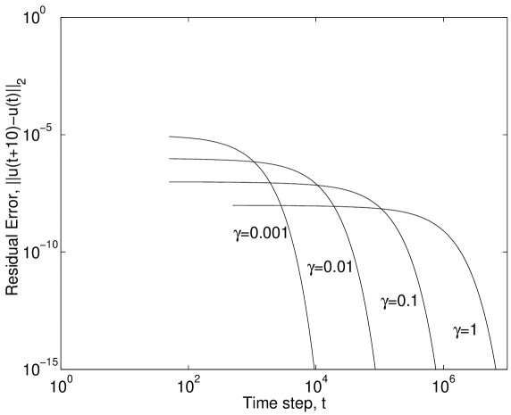
Figure 1: Convergence histories (in log-log scale) of preconditioned MRT-LBE with forcing term for simulation of Poiseuille flow with maximum flow velocity $u_{max}=0.00051$ and kinematic viscosity $\nu=0.001$; $\mbox{\sl Re}=32.6$.

The convergence to steady state is measured by the second-norm of the residual error of the velocity, $||u(t+10)-u(t)||_{2}$. It can be seen that preconditioning the GLBE with forcing term dramatically accelerates the steady state convergence for this problem, in particular, by more than two orders of magnitude with strong preconditioning carried out using $\gamma=0.001$.

Next, we simulate plane Poiseuille flow with relatively higher Ma and Re. As before, we set $L=64$, but use $\nu=0.005$ and apply a pressure gradient such that $\mbox{\sl Ma}=0.00222$ and $\mbox{\sl Re}=163.8$. The convergence history for this problem is presented in Fig. 2.

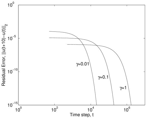
Figure 2: Convergence histories (in log-log scale) of preconditioned MRT-LBE with forcing term for simulation of Poiseuille flow with maximum flow velocity $u_{max}=0.0128$ and kinematic viscosity $\nu=0.005$; $\mbox{\sl Re}=163.8$.

Again, a significant reduction in the number of time steps for convergence to steady state is achieved through preconditioning. On the other hand, it appears that to maintain numerical stability the minimum possible value of the preconditioning parameter $\gamma$ needs to be higher at higher Ma. The computed velocity profile for problem with preconditioning using $\gamma=0.1$ compared with the analytical solution is shown in Fig. 3. Excellent agreement is seen.

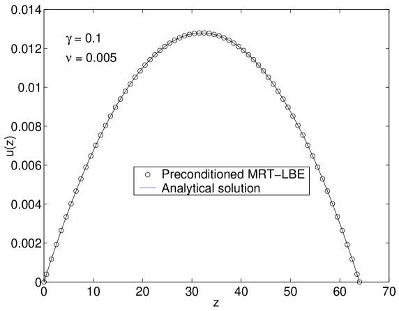
Figure 3: Comparison of computed velocity profile using the preconditioned MRT-LBE with analytical solution for simulation of Poiseuille flow with preconditioning parameter $\gamma=0.1$ and kinematic viscosity $\nu=0.005$; $\mbox{\sl Re}=163.8$

When all the other parameters are maintained constant, the deviation of the computed solution from the analytical solution is related to the ratio $\nu/\gamma$, which, in turn, is related to the hydrodynamic relaxation time in the preconditioned GLBE as $\frac{1}{s_{\nu}^{*}}=3\frac{\nu}{\gamma}+\frac{1}{2}$ (see Sec. 3). Figure 4

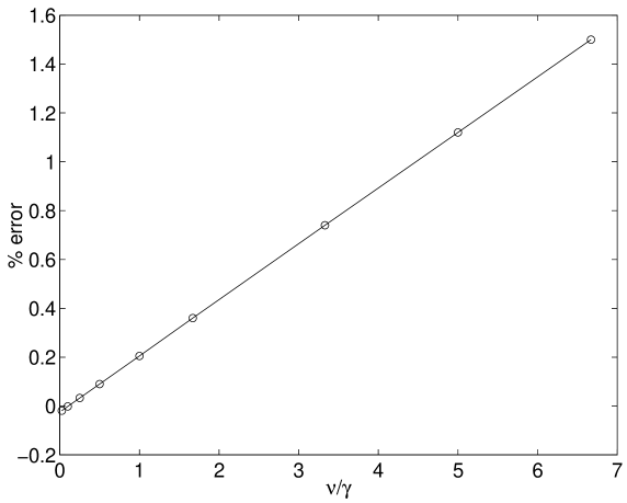
Figure 4: Error in the computed velocity at the center by using the preconditioned MRT-LBE for simulation of Poiseuille flow as a function of the ratio $\nu/\gamma$.

shows the relative error in the computed velocity as a function of $\nu/\gamma$. It is evident that the error, which remains relatively small, is linearly proportional to this ratio. Thus, by maintaining low values of $\nu/\gamma$, the error can be correspondingly kept small.

We now investigate the influence of preconditioning the GLBE on numerical stability for the case of plane Poiseuille flow considered above. This can be done by systematically carrying out simulations at different characteristic parameters, including $\gamma$, $\nu$ and Ma, and determine the threshold at which the computations become unstable, i.e. small variations growing exponentially with time. The results can be conveniently expressed in the form of a regime map or parameter space that delineates stable and unstable parameter sets. Figure 5 shows the stability-instability parameter space determined by the maximum flow velocity $u_{max}$ and the preconditioning parameter $\gamma$ for different fluid viscosity $\nu$.

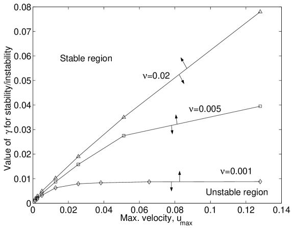
Figure 5: Parameter space of the preconditioning parameter $\gamma$ for stable/unstable computations using the preconditioned MRT-LBE for simulation of Poiseuille flow at different maximum possible flow velocities $u_{max}$ and kinematic viscosities $\nu$ of the fluid.

Arrows normal to the curves pointed upwards indicate stable parameter space, while those pointed downwards pertain to unstable space. This regime map is particularly revealing. First, for a given fluid viscosity $\nu$, as the maximum velocity or, equivalently, Ma is reduced, lower values of the preconditioning parameter $\gamma$ can be used, i.e. the GLBE can be strongly preconditioned resulting in greater computational gains while maintaining numerical stability. The fluid viscosity appears to significantly affect the stability parameter space. For a given $u_{max}$, the minimum possible value of $\gamma$ is higher at higher values of $\nu$. That is, the extent of preconditioning is greater with lower fluid viscosities. Interestingly, Fig. 5 also shows that the delineating curve has a linear functional relationship between $\gamma$ and $u_{max}$ at higher $\nu$, while at lower $\nu$, the stability envelope is nearly flat with a constant $\gamma$ for a wide variation of $u_{max}$. Thus, in general, the benefits of preconditioning, while maintaining numerical stability, is greater at lower Ma and lower $\nu$. It may be noted that the use of GLBE in lieu of SRT-LBE in the context of preconditioning results in significant enhancement of numerical stability, as will be shown later for fully 3D problems characterized by complex fluid motions.

Let us now consider a problem in which we can investigate preconditioning a system of LBE, where the external force impressed on the fluid is a also a strong function of the fluid motion itself. This is, we consider the classical Hartmann flow, consisting of pressure driven flow between two parallel plates in the presence of a magnetic field perpendicular to the walls. In addition to the Reynolds number Re, this problem is characterized by the Hartmann number Ha, which is given by $\mbox{\sl Ha}=B_{0}L\sqrt{\frac{\sigma}{\rho\nu}}$, where $B_{0}$ and $\sigma$ are the applied magnetic field strength and fluid’s electrical conductivity, respectively, and other parameters are as previously defined.

We now simulate this problem by using a vector lattice kinetic scheme preconditioned by parameter $\gamma_{m}$ for magnetic induction (as in Sec. 4), in conjunction with the GLBE with forcing term preconditioned by parameter $\gamma$ (as in Sec. 3). The Lorentz force arising from the interaction of the magnetic induction and velocity field is introduced into consistently preconditioned forcing terms. To simulate the flow of liquid metals at low magnetic Reynolds number $\mbox{\sl Re}_{m}$ or magnetic Prandtl number $\mbox{\sl Pr}_{m}$, we further apply a scaling factor $\chi$ to the preconditioned lattice kinetic scheme (as in Sec. 4.1).

Figure 6 shows the computed steady state velocity profile of Hartmann flow with $\mbox{\sl Re}=286$, $\mbox{\sl Ha}=71.6$, $\mbox{\sl Pr}_{m}=1.0\times 10^{-6}$.

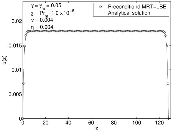
Figure 6: Comparison of computed velocity profile using the preconditioned MRT-LBE with analytical solution for simulation of Hartmann flow with preconditioning parameters $\gamma=\gamma_{m}=0.05$ and kinematic viscosity $\nu=0.004$; $\mbox{\sl Re}=286$, $\mbox{\sl Ha}=71.6$.

This is achieved by using transport coefficients of $\nu=0.004$, and $\eta=0.004$, and $L=64$, along with preconditioning and scaling factors of $\gamma=0.05$, $\gamma_{m}=0.05$ and $\chi=1.0~{}\times~{}10^{-6}$. The corresponding computed steady state magnetic induction profile is presented in Fig. 7.

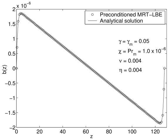
Figure 7: Comparison of computed induced magnetic field profile using the preconditioned MRT-LBE with analytical solution for simulation of Hartmann flow with preconditioning parameters $\gamma=\gamma_{m}=0.05$ and kinematic viscosity $\nu=0.004$; $\mbox{\sl Re}=286$, $\mbox{\sl Ha}=71.6$.

The flattening of the velocity profile observed is characteristic of MHD flows due to the Lorentz force, with most of the velocity variation being confined to the region very close to the wall, in the so-called Hartmann layer. In general, the thickness of Hartmann layer $\delta_{H}$ is inversely proportional to the Hartmann number ($\delta_{H}\sim 1/\mbox{\sl Ha}$). The analytical solution for this problem is provided in standard texts on MHD (e.g., Ref. [54]). It is seen that these profiles computed using preconditioned system of LBE are in excellent agreement with corresponding analytical solutions.

Let us now investigate the behavior of steady state convergence of this problem by applying various levels of preconditioning. Figure 8 shows the convergence history obtained at various values of $\gamma_{m}$ at a fixed value of $\gamma$, i.e. $\gamma=0.05$.

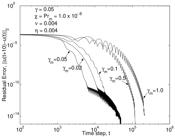
Figure 8: Convergence histories (in log-log scale) of preconditioned MRT-LBE with forcing term in conjunction with preconditioned vector lattice kinetic scheme for simulation of Hartmann flow with flow preconditioning parameter $\gamma=0.05$ for various values of induction preconditioner parameter $\gamma_{m}$; $\mbox{\sl Re}=286$, $\mbox{\sl Ha}=71.6$.

Interestingly, preconditioning only the GLBE with forcing term, but not the vector lattice kinetic scheme (i.e. with $\gamma_{m}=1.0$) results in the slowest convergence. However, as we increase the extent of preconditioning by lowering the values of $\gamma_{m}$, the number of time steps to reach steady state is significantly reduced. The benefits of preconditioning are greatest when both the preconditioning parameters are equal to one another, i.e. $\gamma=\gamma_{m}=0.05$. Moreover, it is also interesting to observe that if the lattice kinetic scheme is more strongly preconditioned than that for the GLBE, i.e. $\gamma_{m}<\gamma$, the approach to steady state becomes slower as compared with the case with $\gamma_{m}=\gamma$. This is consistent with the scaling $O(\mbox{\sl Al})\sim O(\mbox{\sl Ma})$, that is, the propagation speeds of both magnetic field and velocity field by the fluid convective motion occur at similar time scales. Both these are slower than the speed of density perturbation and, thus, preconditioning the terms representing these two physical processes by the same magnitudes would result in the fastest steady state convergence.

This notion is further illuminated by considering cases in which the GLBE is used without preconditioning ($\gamma=1$), while the lattice kinetic scheme is solved with different values of the preconditioning parameter $\gamma_{m}$. The results with these tests are plotted in Fig. 9.

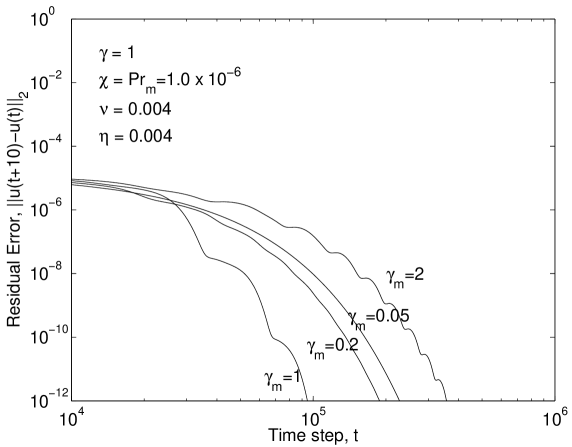
Figure 9: Convergence histories (in log-log scale) of MRT-LBE with forcing term without preconditioning in conjunction with preconditioned vector lattice kinetic scheme for simulation of Hartmann flow with flow preconditioning parameter $\gamma=1.0$ for various values of induction preconditioner parameter $\gamma_{m}$; $\mbox{\sl Re}=286$, $\mbox{\sl Ha}=71.6$.

It shows that the convergence rate actually becomes slower if only one of the LBEs is preconditioned, no matter what the value of the preconditioning parameter is used, when the other LBE is used without preconditioning. Thus, preconditioning should be done for both the LBE and at the same levels. This is further corroborated by considering a series of cases with $\gamma=\gamma_{m}$, as shown in Fig. 10, with lower values for these parameters providing more rapid convergence to steady state.

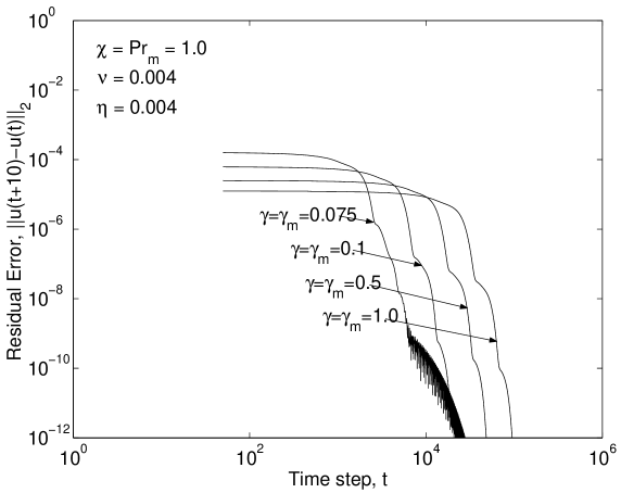
Figure 10: Convergence histories (in log-log scale) of preconditioned MRT-LBE with forcing term in conjunction with preconditioned vector lattice kinetic scheme for simulation of Hartmann flow with equal values of flow ($\gamma$) and induction ($\gamma_{m}$) preconditioning parameters; $\mbox{\sl Re}=286$, $\mbox{\sl Ha}=71.6$.

It may be noted that, in a recent work, we studied a series of problems with very thin Hartmann layers by introducing stretched grids through the Roberts boundary layer transformation [55] by means of an interpolation-supplemented streaming step in the LBE framework [43]. In particular, using this modified LBE, we simulated Hartmann flow with Ha as high as $10,000$ in very good comparison with corresponding asymptotic analytical results, leading to very significant reduction in the number of grid nodes as compared to using standard LBE using uniform grids [43].

We now present some applications of preconditioned LBE for simulation of 3D wall bounded shear flows of electrically conducting fluids such as liquid metals mediated by magnetic fields. In this regard, we consider a cubic cavity of side length $W$ containing liquid metal which is driven by its top lid moving at velocity $U_{0}$. An external magnetic field $B_{0}$ is applied parallel to the lid surface and perpendicular to its direction of motion. A schematic of this flow problem is shown in Fig. 11.

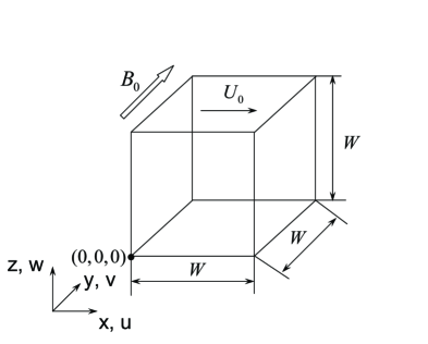
Figure 11: Schematic illustration of a three-dimensional (3D) cubical cavity with its top lid moving at velocity $U_{0}$ in the presence of an external magnetic field $B_{0}$, applied parallel to the lid surface and perpendicular to its direction of motion.

We consider the top lid moving with a velocity $U_{0}=0.0235$ imparting shear on the fluid of viscosity $\nu=0.015$ contained in a cavity discretized by $64^{3}$ grid nodes, such that the Reynolds number is $100$. Initially, we clarify the advantage of preconditioning for this highly 3D flow even for a simpler case that does not involve the application of magnetic field. The velocity boundary conditions at the walls, including the top moving lid, were imposed by using a link bounce back scheme [53]. For the moving wall, this scheme adds contributions due to appropriate momentum to the distribution functions. The convergence histories in the absence of an external magnetic field for different values of $\gamma$ are shown in Fig. 12.

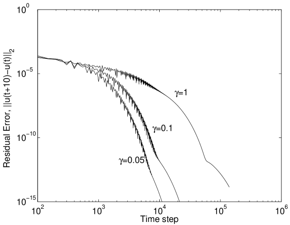
Figure 12: Convergence histories (in log-log scale) of preconditioned MRT-LBE with forcing term for simulation of flow in a 3D cubical driven cavity in the absence of an applied magnetic field with lid velocity $U_{0}=0.0235$ and kinematic viscosity $\nu=0.015$ at different values of flow preconditioning parameters $\gamma$; $\mbox{\sl Re}=100$, grid resolution is $64^{3}$.

It is seen that significant reduction in the number of time steps to reach steady sate, is obtained with preconditioning for this problem.

We now consider the case involving the application of an external magnetic field such that the Hartmann number is $45$, which is obtained by setting $\eta=0.015$, and the magnetic Prandtl number is $5.625\times 10^{-7}$. We consider the induced magnetic fields at far-off distances outside of the cavity to be zero as our boundary condition. This is achieved by considering a larger computational domain for the magnetic induction field encompassing the cavity walls. On these extended computational boundaries, we implement a zero induced field condition through an extrapolation method [56] applied to the vector distribution functions. The corresponding convergence histories for this 3D MHD flow problem are shown in Fig. 13.

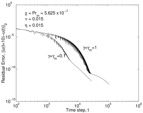
Figure 13: Convergence histories (in log-log scale) of preconditioned MRT-LBE with forcing term for simulation of flow in a 3D cubical driven cavity in the presence of an applied magnetic field with lid velocity $U_{0}=0.0235$ and kinematic viscosity $\nu=0.015$ at different values of preconditioning parameters, with $\gamma=\gamma_{m}$; $\mbox{\sl Re}=100$, $\mbox{\sl Ha}=45$, grid resolution is $64^{3}$.

Again, a significant reduction in the number of time steps to reach steady state is achieved through preconditioning. Moreover, to put things in perspective, when the SRT-LBE was employed for the same grid resolution as above, the simulations were found to be stable only for $\nu\geq 0.166$. On the other hand, with GLBE, as indicated above, we could use a much lower value for $0.015$ while maintaining numerical stability. Thus, for this problem, by using the preconditioned GLBE rather than the preconditioned SRT-LBE, the numerical stability is enhanced by almost an order of magnitude.

We will now investigate the accuracy of preconditioned LBE for this problem. Figures 14, 15 and 16 show the computed velocity profiles for the cases with $\mbox{\sl Ha}=0$ (i.e. no magnetic field) and $\mbox{\sl Ha}=45$ and compared with recent results from simulations carried out using finite-difference method (FDM) involving the solution of the Navier-Stokes equations [57].

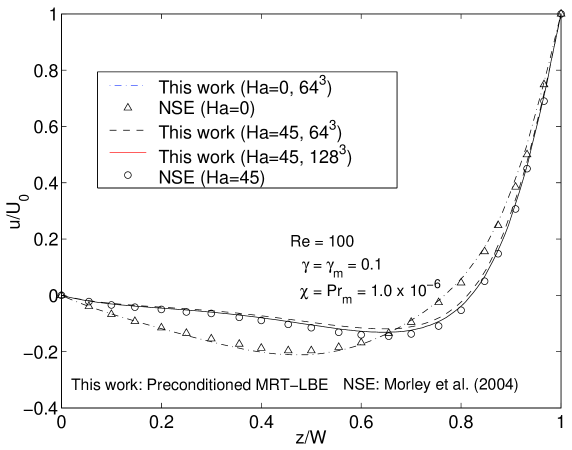
Figure 14: Comparison of computed velocity profile $u$ along the line $x=W/2$ and $y=W/2$ using the preconditioned MRT-LBE with finite-difference solution of NSE (Morley et al. (2004)) for simulation of 3D cubical lid-driven cavity flow with and without magnetic field, i.e., $\mbox{\sl Ha}=0$ and $\mbox{\sl Ha}=45$, respectively; $\mbox{\sl Re}=100$.

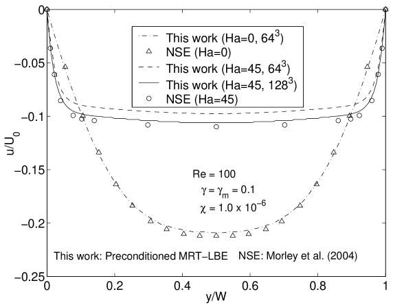
Figure 15: Comparison of computed velocity profile $u$ along the line $x=W/2$ and $z=W/2$ using the preconditioned MRT-LBE with finite-difference solution of NSE (Morley et al. (2004)) for simulation of 3D cubical lid-driven cavity flow with and without magnetic field, i.e., $\mbox{\sl Ha}=0$ and $\mbox{\sl Ha}=45$, respectively; $\mbox{\sl Re}=100$.

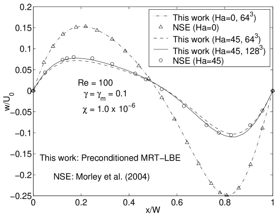
Figure 16: Comparison of computed velocity profile $w$ along the line $y=W/2$ and $z=W/2$ using the preconditioned MRT-LBE with finite-difference solution of NSE (Morley et al. (2004)) for simulation of 3D cubical lid-driven cavity flow with and without magnetic field, i.e., $\mbox{\sl Ha}=0$ and $\mbox{\sl Ha}=45$, respectively; $Re=100$.

The presence of Lorentz forces appears to significantly influence the characteristics of fluid motion in this 3D problem. In particular, the velocity profile appears to be markedly flattened by the presence of magnetic field. The computed results are in excellent agreement with the FDM. It was noticed that the velocity profile bounded by the Hartmann walls (i.e. those perpendicular to the direction of $B_{0}$, see Fig. 11), is somewhat sensitive to the grid resolution employed. Morley et al. [57], who studied this problem using different numerical schemes with different grid resolutions, also observed such effects. In this work, we find that by further refining the grid, i.e. by doubling the number of grid nodes in each direction, the computed solution converges to the FDM results.

For the sake of completeness, we will now consider 3D MHD driven cavity flow with the magnetic field applied in a different manner, i.e. $B_{0}$ perpendicular to the lid surface and its direction of motion as shown in Fig. 17.

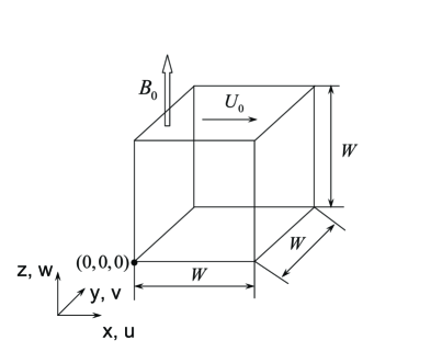
Figure 17: Schematic illustration of a three-dimensional (3D) cubical cavity with its top lid moving at velocity $U_{0}$ in the presence of an external magnetic field $B_{0}$, applied perpendicular to both the lid surface and its direction of motion.

We will consider the effect of magnetic Prandtl number $\mbox{\sl Pr}_{m}$ for this case by employing different values of the scaling factor $\chi$ in the preconditioned LBE. Figures 18, 19 and 20 show the velocity profiles along different directions for $\mbox{\sl Re}=100$, $\mbox{\sl Ha}=45$ with $\gamma=\gamma_{m}=0.1$ for two values of $\mbox{\sl Pr}_{m}$, i.e., $\mbox{\sl Pr}_{m}=5.6\times 10^{-7}$ and $\mbox{\sl Pr}_{m}=1.0$, with the former corresponding to liquid metal.

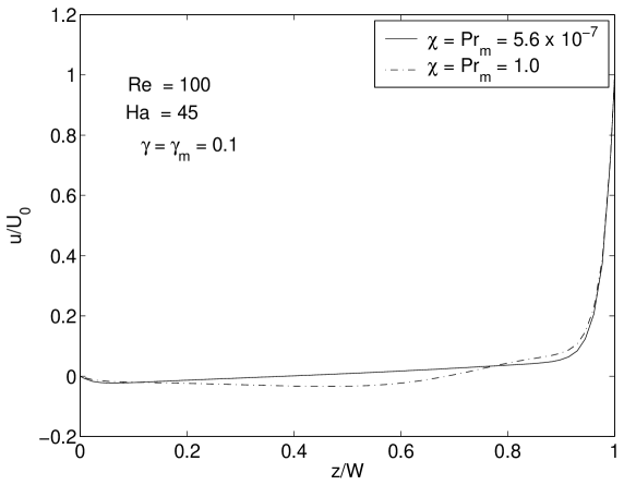
Figure 18: Effect of magnetic Prandtl number $\mbox{\sl Pr}_{m}$ on computed velocity profile $u$ along the line $x=W/2$ and $y=W/2$ for simulation of 3D cubical lid-driven cavity in the presence of magnetic field perpendicular to the lid surface and its direction of motion; $\mbox{\sl Re}=100$ and $\mbox{\sl Ha}=45$.

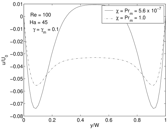
Figure 19: Effect of magnetic Prandtl number $\mbox{\sl Pr}_{m}$ on computed velocity profile $u$ along the line $x=W/2$ and $z=W/2$ for simulation of 3D cubical lid-driven cavity in the presence of magnetic field perpendicular to the lid surface and its direction of motion; $\mbox{\sl Re}=100$ and $\mbox{\sl Ha}=45$.

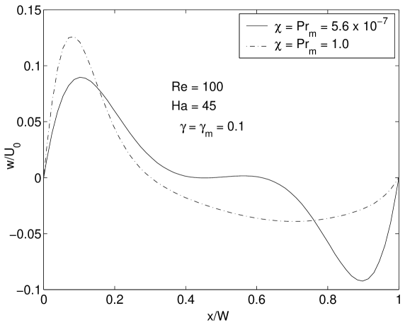
Figure 20: Effect of magnetic Prandtl number $\mbox{\sl Pr}_{m}$ on computed velocity profile $u$ along the line $y=W/2$ and $z=W/2$ for simulation of 3D cubical lid-driven cavity in the presence of magnetic field perpendicular to the lid surface and its direction of motion; $\mbox{\sl Re}=100$ and $\mbox{\sl Ha}=45$.

It is noticed that the values of $\mbox{\sl Pr}_{m}$ appears to strongly modulate the velocity field for those cases in which they are bounded on both sides by stationary walls (Figs. 19 and 20). Moreover, the direction of the application of magnetic field appears to have a profound influence on the flow field. In particular, in contrast to the previous case, we notice the presence of wall jet like features when $B_{0}$ is perpendicular to both the surface of the top lid and its direction of motion (see Fig. 21).

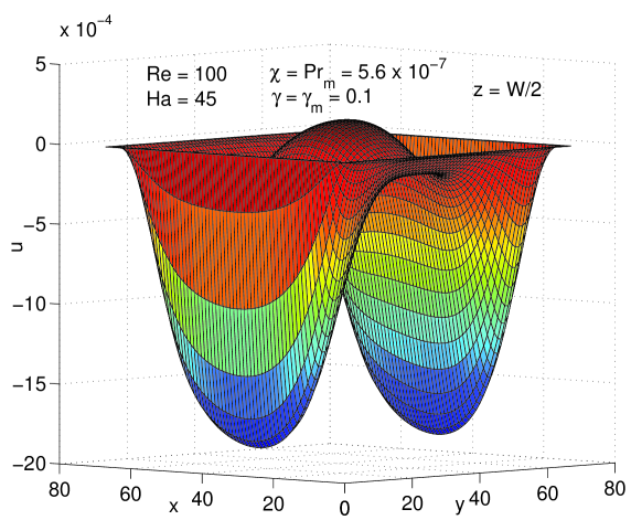
Figure 21: Computed velocity field $u$ along the plane $z=W/2$ showing side wall-jets in a 3D cubical lid-driven cavity in the presence of magnetic field perpendicular to the lid surface and its direction of motion; $\mbox{\sl Re}=100$, $\mbox{\sl Ha}=45$ and $\mbox{\sl Pr}_{m}=5.6\times 10^{-7}$.

6 Summary and Conclusions

In this paper, we devised a preconditioning approach for accelerating the steady state convergence of the solution of the generalized lattice Boltzmann equation (GLBE) with forcing term representing non-uniform force fields. A preconditioning parameter is introduced in the equilibrium moments and in the forcing terms of the GLBE that alleviates the disparity between the propagation speeds of density perturbation and fluid flow processes at low Mach numbers. The use of multiple relaxation times in the collision step involving the solution of the GLBE significantly improves the numerical stability of the approach as compared with the single relaxation time approach. Particular attention is paid to consistently preconditioning the projections of the forcing terms in the natural moment space of the GLBE. In particular, it is shown that to avoid spurious effects due to preconditioning, the slower processes involving the interaction of the velocity field and the external forces need to be preconditioned by the square of the prconditioning parameter. The limiting form of the consistent forcing term, which avoids discrete lattice artifacts particularly for spatially and temporally dependent external forces, is also obtained in the case of SRT-LBE.

As an example of preconditioning an extended system of LBE for complex flows, we also developed a preconditioning procedure for a vector lattice kinetic scheme that accelerate convergence of magnetohydrodynamics (MHD) equations. In the case of MHD flows, there is an additional disparity between the propagation speeds of the perturbation of magnetic induction and the perturbation of the density field, which is mitigated by preconditioning an additional parameter. Motivated by applications in fusion engineering involving handling of liquid metals as blanket walls, in the context of preconditioning, we also devised a simple strategy to simulate flows with low magnetic Reynolds numbers or low magnetic Prandtl numbers. The greatest reduction in the number of time steps to reach steady state is obtained when the preconditioning parameters of both the GLBE and the lattice kinetic scheme are the same. The preconditioned approach yielded solutions in very good agreement with prior solutions for several canonical examples. It is found that the preconditioned LBE reduced the number of steps for steady state convergence between several factors and as much as one or two orders of magnitude depending on the problem. In particular, for 3D MHD cavity flows that are characterized by shear and other complex flow features, the preconditioning approach also yields accurate results in comparison with other numerical solutions. The preconditioning approach presented in this paper can be readily extended for other complex problems such as multiphase flows.

Appendix A Moments, Equilibrium Moments, Moment-projections of Source Terms

A.1 D2Q9 Model

The components of the various elements in the moments are as follows [36]: $\widehat{f}_{0}=\rho,\widehat{f}_{1}=e,\widehat{f}_{2}=e^{2},\widehat{f}_{3}=j_{x},\widehat{f}_{4}=q_{x},\widehat{f}_{5}=j_{y},\widehat{f}_{6}=q_{y},\widehat{f}_{7}=p_{xx},\widehat{f}_{8}=p_{xy}$. Here, $\rho$ is the density, $e$ and $e^{2}$ represent kinetic energy that is independent of density and square of energy, respectively; $j_{x}$ and $j_{y}$ are the components of the momentum, i.e. $j_{x}=\rho u_{x}$ and $j_{y}=\rho u_{y}$, $q_{x}$, and $q_{y}$ are the components of the energy flux, and $p_{xx}$ and $p_{xy}$ are the components of the symmetric traceless viscous stress tensor.

The corresponding components of the equilibrium moments, which are functions of the conserved moments, i.e. density $\rho$ and momentum $\overrightarrow{j}$, are as follows [36]:

$\widehat{f}_{0}^{eq}=\rho,\widehat{f}_{1}^{eq}\equiv e^{eq}=-2\rho+3\frac{\overrightarrow{j}\cdot\overrightarrow{j}}{\rho},\widehat{f}_{2}^{eq}\equiv e^{2,eq}=\rho-3\frac{\overrightarrow{j}\cdot\overrightarrow{j}}{\rho},\widehat{f}_{3}^{eq}=j_{x},\widehat{f}_{4}^{eq}\equiv q_{x}^{eq}=-j_{x},\widehat{f}_{5}^{eq}=j_{y},\widehat{f}_{6}^{eq}\equiv q_{y}^{eq}=-j_{y},\widehat{f}_{7}^{eq}\equiv p_{xx}^{eq}=\frac{(j_{x}^{2}-j_{y}^{2})}{\rho},\widehat{f}_{8}^{eq}\equiv p_{xy}^{eq}=\frac{j_{x}j_{y}}{\rho}$.

The components of the source terms in moment space are functions of external force $\overrightarrow{F}$ and velocity fields $\overrightarrow{u}$, and are given as follows: $\widehat{S}_{0}=0,\widehat{S}_{1}=6(F_{x}u_{x}+F_{y}u_{y}),\widehat{S}_{2}=-6(F_{x}u_{x}+F_{y}u_{y}),\widehat{S}_{3}=F_{x},\widehat{S}_{4}=-F_{x},\widehat{S}_{5}=F_{y},\widehat{S}_{6}=-F_{y},\widehat{S}_{7}=2(F_{x}u_{x}-F_{y}u_{y}),\widehat{S}_{8}=(F_{x}u_{y}+F_{y}u_{x})$.

A.2 D3Q19 Model

The components of the various elements in the moments are as follows [37]: $\widehat{f}_{0}=\rho,\widehat{f}_{1}=e,\widehat{f}_{2}=e^{2},\widehat{f}_{3}=j_{x},\widehat{f}_{4}=q_{x},\widehat{f}_{5}=j_{y},\widehat{f}_{6}=q_{y},\widehat{f}_{7}=j_{z},\widehat{f}_{8}=q_{z},\widehat{f}_{9}=3p_{xx},\widehat{f}_{10}=3\pi_{xx},\widehat{f}_{11}=p_{ww},\widehat{f}_{12}=\pi_{ww},\widehat{f}_{13}=p_{xy},\widehat{f}_{14}=p_{yz},\widehat{f}_{15}=p_{xz},\widehat{f}_{16}=m_{x},\widehat{f}_{17}=m_{y},\widehat{f}_{18}=m_{z}$. Here, $\rho$ is the density, $e$ and $e^{2}$ represent kinetic energy that is independent of density and square of energy, respectively; $j_{x}$, $j_{y}$ and $j_{z}$ are the components of the momentum, i.e. $j_{x}=\rho u_{x}$, $j_{y}=\rho u_{y}$, $j_{z}=\rho u_{z}$, $q_{x}$, $q_{y}$, $q_{z}$ are the components of the energy flux, and $p_{xx}$, $p_{xy}$, $p_{yz}$ and $p_{xz}$ are the components of the symmetric traceless viscous stress tensor; The other two normal components of the viscous stress tensor, $p_{yy}$ and $p_{zz}$, can be constructed from $p_{xx}$ and $p_{ww}$, where $p_{ww}=p_{yy}-p_{zz}$. Other moments include $\pi_{xx}$, $\pi_{ww}$, $m_{x}$, $m_{y}$ and $m_{z}$. The first two of these moments have the same symmetry as the diagonal part of the traceless viscous tensor $p_{ij}$, while the last three vectors are parts of a third rank tensor, with the symmetry of $j_{k}p_{mn}$.

The corresponding components of the equilibrium moments, which are functions of the conserved moments, i.e. density $\rho$ and momentum $\overrightarrow{j}$, are as follows [37]:

$\widehat{f}_{0}^{eq}=\rho,\widehat{f}_{1}^{eq}\equiv e^{eq}=-11\rho+19\frac{\overrightarrow{j}\cdot\overrightarrow{j}}{\rho},\widehat{f}_{2}^{eq}\equiv e^{2,eq}=3\rho-\frac{11}{2}\frac{\overrightarrow{j}\cdot\overrightarrow{j}}{\rho},\widehat{f}_{3}^{eq}=j_{x},\widehat{f}_{4}^{eq}\equiv q_{x}^{eq}=-\frac{2}{3}j_{x},\widehat{f}_{5}^{eq}=j_{y},\widehat{f}_{6}^{eq}\equiv q_{y}^{eq}=-\frac{2}{3}j_{y},\widehat{f}_{7}^{eq}=j_{z},\widehat{f}_{8}^{eq}\equiv q_{z}^{eq}=-\frac{2}{3}j_{z},\widehat{f}_{9}^{eq}\equiv 3p_{xx}^{eq}=\frac{\left[3j_{x}^{2}-\overrightarrow{j}\cdot\overrightarrow{j}\right]}{\rho},\widehat{f}_{10}^{eq}\equiv 3\pi_{xx}^{eq}=3\left(-\frac{1}{2}p_{xx}^{eq}\right),\widehat{f}_{11}^{eq}\equiv p_{ww}^{eq}=\frac{\left[j_{y}^{2}-j_{z}^{2}\right]}{\rho},\widehat{f}_{12}^{eq}\equiv\pi_{ww}^{eq}=-\frac{1}{2}p_{ww}^{eq},\widehat{f}_{13}^{eq}\equiv p_{xy}^{eq}=\frac{j_{x}j_{y}}{\rho},\widehat{f}_{14}^{eq}\equiv p_{yz}^{eq}=\frac{j_{y}j_{z}}{\rho},\widehat{f}_{15}^{eq}\equiv p_{xz}^{eq}=\frac{j_{x}j_{z}}{\rho},\widehat{f}_{16}^{eq}=0,\widehat{f}_{17}^{eq}=0,\widehat{f}_{18}^{eq}=0$.

The components of the source terms in moment space are functions of external force $\overrightarrow{F}$ and velocity fields $\overrightarrow{u}$, and are given as follows [46]:

$\widehat{S}_{0}=0,\widehat{S}_{1}=38(F_{x}u_{x}+F_{y}u_{y}+F_{z}u_{z}),\widehat{S}_{2}=-11(F_{x}u_{x}+F_{y}u_{y}+F_{z}u_{z}),\widehat{S}_{3}=F_{x},\widehat{S}_{4}=-\frac{2}{3}F_{x},\widehat{S}_{5}=F_{y},\widehat{S}_{6}=-\frac{2}{3}F_{y},\widehat{S}_{7}=F_{z},\widehat{S}_{8}=-\frac{2}{3}F_{z},\widehat{S}_{9}=2(2F_{x}u_{x}-F_{y}u_{y}-F_{z}u_{z}),\widehat{S}_{10}=-(2F_{x}u_{x}-F_{y}u_{y}-F_{z}u_{z}),\widehat{S}_{11}=2(F_{y}u_{y}-F_{z}u_{z}),\widehat{S}_{12}=-(F_{y}u_{y}-F_{z}u_{z}),\widehat{S}_{13}=(F_{x}u_{y}+F_{y}u_{x}),\widehat{S}_{14}=(F_{y}u_{z}+F_{z}u_{y}),\widehat{S}_{15}=(F_{x}u_{z}+F_{z}u_{x}),\widehat{S}_{16}=0,\widehat{S}_{17}=0,\widehat{S}_{18}=0$.

Appendix B Chapman-Enskog Analysis of the Preconditioned GLBE with Forcing Term for D2Q9 Model

In this section, by employing the Chapman-Enskog multiscale analysis [48, 39], we derive the macroscopic dynamical equations for the preconditioned GLBE with forcing term corresponding to the D2Q9 model. The analysis of the preconditioned GLBE with other two- or three-dimensional models can be carried out in an analogous way. First, we introduce the expansions

$$\mathbf{\widehat{f}} = \sum_{n=0}^{\infty}\epsilon^{n}\mathbf{\widehat{f}}^{(n)},$$ (37)

$$\partial_{t} = \sum_{n=0}^{\infty}\epsilon^{n}\partial_{t_{n}},$$ (38)

where $\epsilon=\delta_{t}$, along with the Taylor series into the preconditioned GLBE presented in Sec. 3. Then, recognizing that it was derived after making use of the the transformation $\mathbf{\widehat{\overline{f}}}=\mathbf{\widehat{f}}-1/2\mathbf{\widehat{S}}$ on a second-order time discretization of the source terms to make it effectively explicit, and dropping the “overbar” subsequently for convenience, the following equations are obtained as consecutive orders of the parameter $\epsilon$ in moment space (see Ref. [39] for details)

$$O(\epsilon^{0}):\mathbf{\widehat{f}}^{(0)} = \mathbf{\widehat{f}}^{eq,*},$$ (39)

$$O(\epsilon^{1}):\left(\partial_{t_{0}}+\widehat{\mathcal{E}}_{i}\partial_{i}\right)\mathbf{\widehat{f}}^{(0)} = -\widehat{\Lambda}^{*}\mathbf{\widehat{f}}^{(1)}+\mathbf{\widehat{S}}^{*},$$ (40)

$$O(\epsilon^{2}):\partial_{t_{1}}\mathbf{\widehat{f}}^{(0)}+\left(\partial_{t_{0}}+\widehat{\mathcal{E}}_{i}\partial_{i}\right)\left(\mathcal{I}-\frac{1}{2}\widehat{\Lambda}^{*}\right)\mathbf{\widehat{f}}^{(1)} = -\widehat{\Lambda}^{*}\mathbf{\widehat{f}}^{(2)},$$ (41)

where $\widehat{\mathcal{E}}_{i}=\mathcal{T}e_{\alpha i}\mathcal{T}^{-1}$. As it is known that the non-linear terms in the equilibrium moments give rise to slower convective behavior of the fluid as compared with the propagation speed of the density perturbations, we precondition those terms by the parameter $\gamma$ to obtain $\mathbf{\widehat{f}}^{eq,*}$. The forcing terms in moment space are functions of external forces and velocity fields as given in Appendix A. We assume that for the components linear in $\overrightarrow{F}$, we precondition them by $\gamma$. On the other hand, we precondition those that are non-linear due to interactions between $\overrightarrow{F}$ and $\overrightarrow{u}$ by an unknown parameter $\gamma_{1}$, whose form will be deduced as part of the analysis. The final expressions for the preconditioned quantities $\mathbf{\widehat{f}}^{eq,*}$ and $\mathbf{S}^{*}$, as well as $\widehat{\Lambda}^{*}$ are given in Sec. 3.

The components of the first-order equations in moment space, i.e. Eq. (40) can be written as

$$\partial_{t_{0}}\rho+\partial_{x}j_{x}+\partial_{y}j_{y}=0$$ (42)

$$\partial_{t_{0}}\left(-2\rho+\frac{\overrightarrow{j}\cdot\overrightarrow{j}}{\gamma\rho}\right)=-s_{1}^{*}e^{(1)}+6\frac{\overrightarrow{F}\cdot\overrightarrow{u}}{\gamma_{1}}$$ (43)

$$\partial_{t_{0}}\left(\rho-3\frac{\overrightarrow{j}\cdot\overrightarrow{j}}{\gamma\rho}\right)-\overrightarrow{\nabla}\cdot\overrightarrow{j}=-s_{2}^{*}e^{2(1)}-6\frac{\overrightarrow{F}\cdot\overrightarrow{u}}{\gamma_{1}}$$ (44)

$$\partial_{t_{0}}j_{x}+\partial_{x}\left(\frac{1}{3}\rho+\frac{j_{x}^{2}}{\gamma\rho}\right)+\partial_{y}\left(\frac{j_{x}j_{y}}{\gamma\rho}\right)=\frac{F_{x}}{\gamma}$$ (45)

$$\partial_{t_{0}}\left(-j_{x}\right)+\partial_{x}\left(-\frac{1}{3}\rho-\frac{j_{x}^{2}-j_{y}^{2}}{\gamma\rho}\right)+\partial_{y}\left(\frac{j_{x}j_{y}}{\gamma\rho}\right)=-s_{4}^{*}q_{x}^{(1)}-\frac{F_{x}}{\gamma}$$ (46)

$$\partial_{t_{0}}j_{y}+\partial_{x}\left(\frac{j_{x}j_{y}}{\gamma\rho}\right)+\partial_{y}\left(\frac{1}{3}\rho+\frac{j_{y}^{2}}{\gamma\rho}\right)=\frac{F_{y}}{\gamma}$$ (47)

$$\partial_{t_{0}}\left(-j_{y}\right)+\partial_{x}\left(\frac{j_{x}j_{y}}{\gamma\rho}\right)+\partial_{y}\left(-\frac{1}{3}\rho+\frac{j_{x}^{2}-j_{y}^{2}}{\gamma\rho}\right)=-s_{6}^{*}q_{y}^{(1)}-\frac{F_{y}}{\gamma}$$ (48)

$$\partial_{t_{0}}\left(\frac{j_{x}^{2}-j_{y}^{2}}{\gamma\rho}\right)+\partial_{x}\left(\frac{2}{3}j_{x}\right)-\partial_{y}\left(\frac{2}{3}j_{y}\right)=-s_{7}^{*}p_{xx}^{(1)}+2\frac{F_{x}u_{x}-F_{y}u_{y}}{\gamma_{1}}$$ (49)

$$\partial_{t_{0}}\left(\frac{j_{x}j_{y}}{\gamma\rho}\right)+\partial_{x}\left(\frac{1}{3}j_{x}\right)+\partial_{y}\left(\frac{1}{3}j_{y}\right)=-s_{8}^{*}p_{xy}^{(1)}+\frac{F_{x}u_{y}+F_{y}u_{x}}{\gamma_{1}}$$ (50)

Similarly, the components of the second-order equations in moment space, i.e. Eq. (41) are

$$\partial_{t_{1}}\rho=0$$ (51)

$$\partial_{t_{1}}\left(-2\rho+\frac{\overrightarrow{j}\cdot\overrightarrow{j}}{\gamma\rho}\right)+\partial_{t_{0}}\left(\left[1-\frac{1}{2}s_{1}^{*}\right]e^{(1)}\right)+$$

$$\partial_{x}\left(\left[1-\frac{1}{2}s_{4}^{*}\right]q_{x}^{(1)}\right)+\partial_{y}\left(\left[1-\frac{1}{2}s_{6}^{*}\right]q_{y}^{(1)}\right)=-s_{1}^{*}e^{(2)}$$ (52)

$$\partial_{t_{1}}\left(\rho-3\frac{\overrightarrow{j}\cdot\overrightarrow{j}}{\gamma\rho}\right)+\partial_{t_{0}}\left(\left[1-\frac{1}{2}s_{2}^{*}\right]e^{2(1)}\right)+$$

$$\partial_{x}\left(\left[1-\frac{1}{2}s_{4}^{*}\right]q_{x}^{(1)}\right)+\partial_{y}\left(\left[1-\frac{1}{2}s_{6}^{*}\right]q_{y}^{(1)}\right)=-s_{2}^{*}e^{2(2)}$$ (53)

$$\partial_{t_{1}}j_{x}+\partial_{x}\left(\frac{1}{6}\left[1-\frac{1}{2}s_{1}^{*}\right]e^{(1)}+\frac{1}{2}\left[1-\frac{1}{2}s_{7}^{*}\right]p_{xx}^{(1)}\right)+$$

$$\partial_{y}\left(\left[1-\frac{1}{2}s_{8}^{*}\right]p_{xy}^{(1)}\right)=0$$ (54)

$$\partial_{t_{1}}\left(-j_{x}\right)+\partial_{t_{0}}\left(\left[1-\frac{1}{2}s_{4}^{*}\right]q_{x}^{(1)}\right)+$$

$$\partial_{x}\left(\frac{1}{3}\left[1-\frac{1}{2}s_{1}^{*}\right]e^{(1)}+\frac{1}{3}\left[1-\frac{1}{2}s_{2}^{*}\right]e^{2(1)}-\left[1-\frac{1}{2}s_{7}^{*}\right]p_{xx}^{(1)}\right)+$$

$$\partial_{y}\left(\left[1-\frac{1}{2}s_{8}^{*}\right]p_{xy}^{(1)}\right)=-s_{4}^{*}q_{x}^{(2)}$$ (55)

$$\partial_{t_{1}}j_{y}+\partial_{x}\left(\left[1-\frac{1}{2}s_{8}^{*}\right]p_{xy}^{(1)}\right)+$$

$$\partial_{y}\left(\frac{1}{6}\left[1-\frac{1}{2}s_{1}^{*}\right]e^{(1)}-\frac{1}{2}\left[1-\frac{1}{2}s_{7}^{*}\right]p_{xx}^{(1)}\right)=0$$ (56)

$$\partial_{t_{1}}\left(-j_{y}\right)+\partial_{t_{0}}\left(\left[1-\frac{1}{2}s_{6}^{*}\right]q_{y}^{(1)}\right)+\partial_{x}\left(\left[1-\frac{1}{2}s_{8}^{*}\right]p_{xy}^{(1)}\right)+$$

$$\partial_{y}\left(\frac{1}{3}\left[1-\frac{1}{2}s_{1}^{*}\right]e^{(1)}+\frac{1}{3}\left[1-\frac{1}{2}s_{2}^{*}\right]e^{2(1)}+\left[1-\frac{1}{2}s_{7}^{*}\right]p_{xx}^{(1)}\right)=-s_{6}^{*}q_{y}^{(2)}$$ (57)

$$\partial_{t_{1}}\left(\frac{j_{x}^{2}-j_{y}^{2}}{\gamma\rho}\right)+\partial_{t_{0}}\left(\left[1-\frac{1}{2}s_{7}^{*}\right]p_{xx}^{(1)}\right)+$$

$$\partial_{x}\left(-\frac{1}{3}\left[1-\frac{1}{2}s_{4}^{*}\right]q_{x}^{(1)}\right)+\partial_{y}\left(\frac{1}{3}\left[1-\frac{1}{2}s_{6}^{*}\right]q_{y}^{(1)}\right)=-s_{7}^{*}p_{xx}^{(2)}$$ (58)

$$\partial_{t_{1}}\left(\frac{j_{x}j_{y}}{\gamma\rho}\right)+\partial_{t_{0}}\left(\left[1-\frac{1}{2}s_{8}^{*}\right]p_{xy}^{(1)}\right)+$$

$$\partial_{x}\left(\frac{1}{3}\left[1-\frac{1}{2}s_{6}^{*}\right]q_{y}^{(1)}\right)+\partial_{y}\left(\frac{1}{3}\left[1-\frac{1}{2}s_{4}^{*}\right]q_{x}^{(1)}\right)=-s_{8}^{*}p_{xy}^{(2)}$$ (59)

To obtain preconditioned hydrodynamical equations, we need to combine the evolution equations of moments corresponding to Eqs. (42), (45) and (47) with Eqs. (51), (54) and (56), respectively. Inspection of these six equations show that we need explicit expressions for the following non-equilibrium moments: $e^{(1)}$, $p_{xx}^{(1)}$ and $p_{xy}^{(1)}$. Thus, from Eqs. (43), (49) and (50), we get

$$e^{(1)}=\frac{1}{s_{1}^{*}}\left[-\partial_{t_{0}}\left(-2\rho+3\frac{\overrightarrow{j}\cdot\overrightarrow{j}}{\gamma\rho}\right)+6\frac{\overrightarrow{F}\cdot\overrightarrow{u}}{\gamma_{1}}\right]$$ (60)

$$p_{xx}^{(1)}=\frac{1}{s_{6}^{*}}\left[-\partial_{t_{0}}\left(\frac{j_{x}^{2}-j_{y}^{2}}{\gamma\rho}\right)-\partial_{x}\left(\frac{2}{3}j_{x}\right)+\partial_{y}\left(\frac{2}{3}j_{y}\right)+2\frac{\left(F_{x}u_{x}-F_{y}u_{y}\right)}{\gamma_{1}}\right]$$ (61)

$$p_{xy}^{(1)}=\frac{1}{s_{7}^{*}}\left[-\partial_{t_{0}}\left(\frac{j_{x}j_{y}}{\gamma\rho}\right)-\partial_{x}\left(\frac{1}{3}j_{x}\right)-\partial_{y}\left(\frac{1}{3}j_{y}\right)+\frac{\left(F_{x}u_{y}+F_{y}u_{x}\right)}{\gamma_{1}}\right]$$ (62)

Eqs. (60)-(62) require time derivatives of the density and velocity (or momentum) fields, which can be obtained from Eqs. (42), (45) and (47) and truncating terms of $O(\mbox{\sl Ma}^{2})$ or higher. Thus, we have

$\partial_{t_{0}}\left(\frac{j_{x}^{2}}{\rho}\right)\approx 2\frac{F_{x}u_{x}}{\gamma},\qquad\partial_{t_{0}}\left(\frac{j_{y}^{2}}{\rho}\right)\approx 2\frac{F_{y}u_{y}}{\gamma},\qquad\partial_{t_{0}}\left(\frac{j_{x}j_{y}}{\rho}\right)\approx 2\frac{\left(F_{x}u_{y}+F_{y}u_{x}\right)}{\gamma}$

Substituting the above relations in Eq. (60)

$$e^{(1)}=\frac{1}{s_{1}^{*}}\left[-2\overrightarrow{\nabla}\cdot\overrightarrow{j}-3\left(\frac{2\frac{F_{x}u_{x}}{\gamma}+2\frac{F_{y}u_{y}}{\gamma}}{\gamma}\right)+6\frac{\overrightarrow{F}\cdot\overrightarrow{u}}{\gamma_{1}}\right]$$ (63)

In order to eliminate the dependence of forcing terms in the above equation, Eq. (63), so that the macrodynamical equations recover correct physics without any spurious effects, we need to set

$$\gamma_{1}=\gamma^{2}.$$ (64)

Thus, Eq. (64) suggests that the moment projections of forcing terms involving non-linear interactions of external force and velocity fields should be preconditioned by a factor of $1/\gamma^{2}$, as they represent slower physical processes than fluid flow itself. Hence, we get

$$e^{(1)}=-2\frac{1}{s_{1}^{*}}\overrightarrow{\nabla}\cdot\overrightarrow{j}.$$ (65)

Similarly,

$$p_{xx}^{(1)}=-\frac{2}{3}\frac{1}{s_{7}^{*}}\left(\partial_{x}j_{x}-\partial_{y}j_{y}\right),$$ (66)

and

$$p_{xy}^{(1)}=-\frac{1}{3}\frac{1}{s_{8}^{*}}\left(\partial_{x}j_{y}+\partial_{y}j_{x}\right).$$ (67)

So, the preconditioned dynamical equations of the conserved moments are finally obtained by adding Eqs. (42), (45) and (47) to Eqs. (51), (54) and (56), respectively, after multiplying the latter with $\delta_{t}$, and using Eqs. (65)-(67). They correspond to the following preconditioned weakly compressible Navier-Stokes equations

$$\partial_{t}\rho+\partial_{x}j_{x}+\partial_{y}j_{y}=0$$ (68)

$$\partial_{t}j_{x}+\frac{1}{\gamma}\left[\partial_{x}\left(\frac{j_{x}^{2}}{\rho}\right)+\partial_{y}\left(\frac{j_{x}j_{y}}{\rho}\right)\right]=-\frac{1}{\gamma}\partial_{x}p+$$

$$\frac{1}{\gamma}\partial_{x}\left(2\nu\left[\partial_{x}j_{x}-1/3\overrightarrow{\nabla}\cdot\overrightarrow{j}\right]+\zeta\overrightarrow{\nabla}\cdot\overrightarrow{j}\right)+$$

$$\frac{1}{\gamma}\partial_{y}\left(\nu\left[\partial_{x}j_{y}+\partial_{y}j_{x}\right]\right)+\frac{F_{x}}{\gamma}$$ (69)

$$\partial_{t}j_{y}+\frac{1}{\gamma}\left[\partial_{x}\left(\frac{j_{x}j_{y}}{\rho}\right)+\partial_{y}\left(\frac{j_{y}^{2}}{\rho}\right)\right]=-\frac{1}{\gamma}\partial_{y}p+$$

$$\frac{1}{\gamma}\partial_{x}\left(\nu\left[\partial_{x}j_{y}+\partial_{y}j_{x}\right]\right)+$$

$$\frac{1}{\gamma}\partial_{y}\left(2\nu\left[\partial_{y}j_{y}-1/3\overrightarrow{\nabla}\cdot\overrightarrow{j}\right]+\zeta\overrightarrow{\nabla}\cdot\overrightarrow{j}\right)+\frac{F_{y}}{\gamma}$$ (70)

where the pressure field $p$ is given by

$$p=\gamma\frac{1}{3}\rho$$ (71)

and the transport coefficients, viz., the bulk and shear viscosities, respectively, as

$$\zeta=\gamma\frac{1}{3}\left[\frac{1}{s_{1}^{*}}-\frac{1}{2}\right]\delta_{t}$$ (72)

and

$$\nu=\gamma\frac{1}{3}\left[\frac{1}{s_{\beta}^{*}}-\frac{1}{2}\right]\delta_{t},\quad\beta=7,8$$ (73)

Appendix C Chapman-Enskog Analysis of the Preconditioned Vector Kinetic Equation

We now perform the Chapman-Enskog analysis of the preconditioned vector kinetic equation by introducing the expansions

$$g_{\alpha i} = \sum_{n=0}^{\infty}\epsilon^{n}g_{\alpha i}^{(n)},$$ (74)

$$\partial_{t} = \sum_{n=0}^{\infty}\epsilon^{n}\partial_{t_{n}},$$ (75)

with $\epsilon=\delta_{t}$, in conjunction with the Taylor series [48, 51], which result in the following:

$$O(\epsilon^{0}):g_{\alpha i}^{(0)} = g_{\alpha i}^{eq,*},$$ (76)

$$O(\epsilon^{1}):\left(\partial_{t_{0}}+e_{\alpha j}\partial_{j}\right)g_{\alpha i}^{(0)} = -\frac{1}{\tau_{m}^{*}}g_{\alpha i}^{(1)},$$ (77)

$$O(\epsilon^{2}):\partial_{t_{1}}g_{\alpha i}^{(0)}+\left(1-\frac{1}{2\tau_{m}^{*}}\right)\left(\partial_{t_{0}}+e_{\alpha j}\partial_{j}\right)g_{\alpha i}^{(1)} = -\frac{1}{\tau_{m}^{*}}g_{\alpha i}^{(2)}.$$ (78)

Now, using the following summational constraints $\sum_{\alpha=0}^{b_{m}}g_{\alpha j}^{(0)}=B_{j}$, $\sum_{\alpha=0}^{b_{m}}e_{\alpha i}g_{\alpha j}^{(0)}=\Lambda_{ij}^{(0)}$, $\sum_{\alpha=0}^{b_{m}}g_{\alpha j}^{(n)}=0$ and $\sum_{\alpha=0}^{b_{m}}e_{\alpha i}g_{\alpha j}^{(n)}=\Lambda_{ij}^{(n)}$ for $n\geq 1$, with $\Lambda_{ij}^{(0)}=\frac{u_{i}B_{j}-B_{i}u_{j}}{\gamma_{m}}$, and taking zeroth moments of Eqs. (77) and (78), we get

$$\partial_{t_{0}}B_{i}+\partial_{j}\Lambda_{ji}^{(0)} = 0,$$ (79)

$$\partial_{t_{1}}B_{i}+\left(1-\frac{1}{2\tau_{m}^{*}}\right)\partial_{j}\Lambda_{ji}^{(1)} = 0.$$ (80)

Taking the first moment, i.e. $\sum_{\alpha=0}^{b_{m}}e_{\alpha j}(\cdot)$ of Eq. (77) and using the identity $\sum_{\alpha=0}^{b_{m}}e_{\alpha j}e_{\alpha k}g_{\alpha i}^{(0))}=\theta_{m}\delta_{jk}B_{i}$, where $\delta_{jk}$ is the Kronecker delta, we get

$$\Lambda_{ji}^{(1)}=-\tau_{m}^{*}\left[\partial_{t_{0}}\Lambda_{ji}^{(0)}+\theta_{m}\partial_{j}B_{i}\right].$$ (81)

With the scaling $O(B_{i})\sim O(u_{i})$ [51] and considering the zeroth-order momentum and magnetic induction equations, $\partial_{t_{0}}\Lambda_{ji}^{(0)}\sim O(\mbox{\sl Ma}^{3})$ and hence can be neglected. As a result,

$$\Lambda_{ji}^{(1)}\approx-\tau_{m}^{*}\theta_{m}\partial_{j}B_{i}.$$ (82)

Finally, adding Eq. (79) and Eq. (80)$\times\delta_{t}$ and using $\partial_{t}\approx\partial_{t_{0}}+\delta_{t}\partial_{t_{1}}$, along with Eq. (82), we get the preconditioned magnetic induction equation

$$\partial_{t}B_{i}+\frac{1}{\gamma_{m}}\nabla_{j}\left(u_{j}B_{i}-B_{j}u_{i}\right)=\frac{1}{\gamma_{m}}\partial_{j}\left(\eta\partial_{j}B_{i}\right),$$ (83)

where $\eta=\gamma_{m}\theta_{m}\left(\tau_{m}^{*}-1/2\right)\delta_{t}$.

References

- [1] S. Chen and G. Doolen, Lattice Boltzmann method for fluid flows, Annu. Rev. Fluid Mech. 8 (1998) 2527.
- [2] S. Succi, The Lattice Boltzmann Equation for Fluid Dynamics and Beyond, Clarendon Press, Oxford (2001).
- [3] X. Shan and H. Chen, Lattice Boltzmann model for simulating flows with multiple phases and components, Phys. Rev. E 47 (1993) 1815.
- [4] M. Swift, E. Orlandini, W. Obsborn and J. Yeomans, Lattice Boltzmann simulations of liquid-gas and binary fluid systems, Phys. Rev. E 54 (1996) 5041.
- [5] F. J. Higuera, S. Succi and R. Benzi, Lattice gas-dynamics with enhanced collisions, Europhys. Lett. 9 (1989) 345.
- [6] X. He and L.S. Luo, A priori derivation of the lattice Boltzmann equation, Phys. Rev. E 55 (1997) 115.
- [7] T. Abe, Derivation of the lattice Boltzmann method by means of the discrete ordinate method for the Boltzmann equation, J. Comp. Phys. 131 (1997) 241.
- [8] L.S. Luo, Theory of the lattice Boltzmann method: Lattice Boltzmann models for nonideal gases, Phys. Rev. E 62 (2000) 4982.
- [9] X. He and G. Doolen, Thermodynamic foundations of kinetic theory and Lattice Boltzmann Models for Multiphase Flows, J. Stat. Phys. 107 (2002) 1572.
- [10] P. Asinari, Semi-implicit-linearized multiple-relaxation-time formulation of lattice Boltzmann schemes for mixture modeling, Phys. Rev. E 73 (2006) 056705.
- [11] M. Junk, A. Klar and L.S. Luo, Asymptotic analysis of the lattice Boltzmann equation, J. Comp. Phys. 210 (2005) 676.
- [12] A.J.C. Ladd and R. Verberg, Lattice-Boltzmann simulations of particle-fluid suspensions, J. Stat. Phys. 104 (2001) 1191.
- [13] S. Succi, I. Karlin and H. Chen, Role of the H theorem in lattice Boltzmann hydrodynamic simulations, Rev. Mod. Phys. 74 (2002) 1203.
- [14] D. Yu , R. Mei, L.-S. Luo and W. Shyy, Viscous flow computations with the method of lattice Boltzmann equation, Progress in Aerospace Sciences 39 (2003) 329.
- [15] R.R. Nourgaliev, T.N. Dinh, T.G. Theofanous and D. Joseph, The lattice Boltzmann equation method: Theoretical interpretation, numerics and implications, Int. J. Multiphase Flow 29 (2003) 117.
- [16] K.N. Premnath, M.E. McCracken and J. Abraham, A review of lattice Boltzmann methods for multiphase flow relevant to engine sprays, Trans. SAE: J. Engines 113 (2005) 929.
- [17] R. Leveque, Finite Volume Method for Hyperbolic Problems, Cambridge University Press, New York (2002).
- [18] R. Verberg and A.J.C. Ladd, Simulation of low-Reynolds-number flow via a time-independent lattice-Boltzmann method, Phys. Rev. E 60 (1999) 3366.
- [19] M. Bernaschi, S. Succi and H. Chen, Accelerated lattice Boltzmann schemes for steady-state flow simulations, J. Sci. Comp. 16 (2001) 135.
- [20] J. Tölke, M. Krafczyk and E. Rank, A multigrid-solver for the discrete Boltzmann equation, J. Stat. Phys. 107 (2002) 573.
- [21] D. Kandhai, A. Koponen, A. Hoekstra and P.M.A. Sloot, Iterative momentum relaxation for fast lattice-Boltzmann simulations, Future Gen. Comput. Sys. 18 (2001) 89.
- [22] T. Lee and C.L. Lin, An Eulerian description of the streaming process in the lattice Boltzmann equation, J. Comp. Phys. 185 (2003) 471.
- [23] T. Seta and R. Takahashi, Numerical stability analysis of FDLBM, J. Stat. Phys. 107 (2002) 1572.
- [24] J. Tölke, M. Krafczyk, M. Schulz and E. Rank, Implicit discretization and nonuniform mesh refinement approaches for FD discretization of LBGK models, Int. J. Mod. Phys. C 9 (1998) 1143.
- [25] D. Mavriplis, Multigrid solution of the steady-state lattice Boltzmann equation, Comp. Fluids 35 (2006) 793.
- [26] Z. Guo, T.S. Zhao and Y. Shi, Preconditioned lattice-Boltzmann method for steady flows, Phys. Rev. E 70 (2004) 066706.
- [27] E. Turkel, Preconditioning methods for solving the incompressible and low speed compressible equations J. Comp. Phys. 72 (1987) 277.
- [28] B. van Leer, W.T. Lee and P.L. Roe, Characteristic time-stepping for local preconditioning of the Euler equations in AIAA 10th Computational Fluid Dynamics Conference (1991).
- [29] D. Choi and C.L. Merkle, The application of preconditioning to viscous flows J. Comp. Phys. 105 (1993) 207.
- [30] E. Turkel, Preconditioning techniques in computational fluid dynamics Annu. Rev. Fluid Mech. 31 (1999) 385.
- [31] P.L. Bhatnagar, E.P. Gross and M. Krook, A model for collision processes in gases. I. Small amplitude processes in charged in neutral one-component systems, Phys. Rev. E 94 (1954) 511.
- [32] S. Izquierdo and N. Fueyo, Preconditioned Navier-Stokes schemes from the generalized lattice Boltzmann equation, Prog. Comput. Fluid Dyn. 8 (2008) 189.
- [33] Y. Qian, D. d’Humiéres and P. Lallemand, Lattice BGK models for Navier-Stokes equations, Europhys. Lett. 17 (1992) 479.
- [34] H. Chen, S. Chen and W.H. Matthaeus, Recovery of the Navier-Stokes equations using a lattice-gas Boltzmann method, Phys. Rev. A 45 (1992) R5339.
- [35] D. d’Humiéres, Generalized lattice Boltzmann equations, Progress in Aeronautics and Astronautics (Eds. B.D. Shigal and D.P. Weaver) Washington D.C. 450(1992).
- [36] P. Lallemand and L.-S. Luo, Theory of the lattice Boltzmann method: Dispersion, dissipation, isotropy, Galilean invariance, and stability, Phys. Rev. E 61 (2000) 6546.
- [37] D. d’Humiéres, I. Ginzburg, M. Krafczyk, P. Lallemand and L.-S. Luo, Multiple-Relaxation-Time lattice Boltzmann models in three-dimensions, Phil. Trans. Roy. Soc. London: Series A 360 (2002) 437.
- [38] M.E. McCracken and J. Abraham, Multiple-Relaxation-Time lattice-Boltzmann model for multiphase flow, Phys. Rev. E 71 (2005) 036701.
- [39] K.N. Premnath and J. Abraham, Three-dimensional Multi-Relaxation Time (MRT) lattice-Boltzmann models for multiphase flow, J. Comp. Phys. 224 (2007) 539.
- [40] K.N. Premnath and J. Abraham, Simulations of binary drop collisions with a Multiple-Relaxation-Time lattice-Boltzmann model, Phys. Fluids 17 (2005) 122105.
- [41] M.E. McCracken and J. Abraham, Simulations of liquid break up with an axisymmetric, multiple relaxation time, index-function lattice Boltzmann model, Int. J. Mod. Phys. C 16 (2005) 1671.
- [42] J. Tölke, S. Freudiger and M. Krafczyk, An adaptive scheme for LBE multiphase flow simulations on hierarchical grids, Comp. Fluids 35 (2006) 820.
- [43] M.J. Pattison, K.N. Premnath, N.B. Morley and M. Abdou, Progress in lattice Boltzmann methods for magnetohydrodynamic flows relevant to fusion applications, Fusion Engg. Des. 83 (2008) 557.
- [44] M. Krafczyk, J. Tölke and L.-S. Luo, Large-eddy simulations with a Multiple-Relaxation-Time LBE model, Int. J. Mod. Phys. B 17 (2003) 33.
- [45] H. Yu, L.-S. Luo and S.S. Girimaji, LES of turbulent square jet flow using an MRT lattice Boltzmann model, Comp. Fluids 35 (2006) 957.
- [46] K.N. Premnath, M.J. Pattison and S. Banerjee, Generalized lattice Boltzmann equation with forcing term for Computation of Wall Bounded Turbulent Flows, Phys. Rev. E, submitted (2008).
- [47] X. He, L.-S. Luo and M. Dembo, Some progress in the lattice Boltzmann method: Reynolds number enhancement in simulations, Physica A 239 (2006997) 276.
- [48] S. Chapman and T.G. Cowling, Mathematical Theory of Nonuniform Gases, Cambridge University Press, New York (1964).
- [49] X. He, X. Shan and G.D. Doolen, A Discrete Boltzmann Equation Model for Non-Ideal Gases, Phys. Rev. E 57 (1998) R13.
- [50] Z. Guo, C. Zheng and B. Shi, Discrete lattice effects on the forcing term in the lattice Boltzmann method, Phys. Rev. E 65 (2002) 046308.
- [51] P.J. Dellar, Lattice kinetic schemes for magnetohydrodynamics, J. Comp. Phys. 179 (2002) 95.
- [52] G. Breyiannis and D. Valougeorgis, Lattice Boltzmann simulations in 3-D magnetohydrodynamics, Phys. Rev. E 69 (2004) 065702.
- [53] A.J.C. Ladd, Numerical simulations of particulate suspensions via a discretized Boltzmann equation, J. Fluid Mech. 271 (1994) 285.
- [54] U. Müller and L. Bühler, Magnetohydrodynamics in Channels and Containers, Springer, New York (2001).
- [55] G.O. Roberts, Computational meshes for boundary layer problems, Second Int. Conf. Numer. Meth. Fluid Dyn., Lect. Notes Phys. 8 (1971) 171.
- [56] S. Chen, D. Martinez, and R. Mei, On Boundary conditions in lattice Boltzmann method, Phys. Fluids 8 (1996) 2527.
- [57] N.B. Morley, S. Smolentsev, R. Munipalli, M. Ni, D. Gao and M. Abdou, Progress on the modeling of liquid metal, free surface, MHD flows for fusion liquid walls Fusion Engg. Des. 72 (2004) 3.