The Impact of Neutrino Magnetic Moments on the Evolution of Massive Stars
Abstract
We explore the sensitivity of massive stars to neutrino magnetic moments. We find that the additional cooling due to the neutrino magnetic moments bring about qualitative changes to the structure and evolution of stars in the mass window , rather than simply changing the time scales for the burning. We describe some of the consequences of this modified evolution: the shifts in the threshold masses for creating core-collapse supernovae and oxygen-neon-magnesium white dwarfs and the appearance of a new type of supernova in which a partial carbon-oxygen core explodes within a massive star. The resulting sensitivity to the magnetic moment is at the level of .
Subject headings:
neutrinos — stars: supergiants — stars: evolution — stars: interiors1. Introduction
Cooling by neutrino emission is known to be important in a variety of stellar systems, from low-mass red giants (RG) and horizontal branch (HB) stars to white dwarfs (WD), neutron stars and core-collapse supernovae (CCSN). Although, compared with photons, neutrinos interact extremely weakly, once produced they easily escape from stellar interiors carrying away energy that would otherwise take much longer to be transported to the surface by radiation or convection. The resulting energy sink in the center of the star can dictate the star’s rate of nuclear burning, structure and evolution, and ultimately how it ends its life. If a new interaction modifies the rate at which neutrinos are produced, the evolution of the star could change. Stars can therefore be used as laboratories to search for non-standard properties of the neutrino (Bernstein et al., 1963).
One such new interaction that will be considered in this paper are the neutrino (transition) magnetic moments. The magnetic moments couple neutrinos to photon through the effective Lagrangian term
| (1) |
where is the neutrino field, the electromagnetic field tensor, , are Lorentz indices, , are the flavor indices. This interaction is non-zero, although extremely small, already in the Standard Model (SM) with non-zero neutrino mass. In some extensions of the SM it is allowed to be as large as the present direct laboratory bound of (Daraktchieva et al., 2005), where is the Bohr magneton (see Sect. 2.1). Such new physics could reside just above the electroweak scale of .
The effects of the magnetic moment interaction on the evolution of low-mass stars have been extensively studied, as will be reviewed in Sect. 2 (see also, e.g., Raffelt 1996, 1999, 2000 for a review). In fact, these stars are thought to give the best bound on the neutrino magnetic moment, about an order of magnitude more restrictive than the direct laboratory bound. The effect of the magnetic moment on the evolution of massive () stars, however, has not been established. This paper is an exploratory investigation designed to fill this gap. Our goal is to answer the following questions:
-
•
Does the presence of a non-vanishing neutrino magnetic moment influence in any way the behavior of a massive star?
-
•
If so, for which range of stellar masses?
-
•
What are the induced effects?
-
•
What is the sensitivity of massive stars to the size of the neutrino magnetic moment?
The paper is organized as follows: In Sect. 2, we discuss the neutrino magnetic moments from the theoretical and phenomenological points of view. In particular, we review the present bounds from experiments and astrophysical considerations. In Sect. 3, we review the standard evolution of massive stars and consider how might change with the addition of the extra cooling induced by a non-zero . In Sect. 4, we present the results of our numerical modeling. Finally in Sect. 5, we summarize our results and discuss possible future directions.
2. Neutrino Magnetic Moment
2.1. Theoretical considerations
The search for the neutrino magnetic moment goes back to the neutrino discovery experiment by Cowan & Reines (1957), who put the first bound on the magnetic moment,
On the theoretical front, it was realized many decades ago that a neutrino with a non-zero mass should have a non-vanishing magnetic moment even with the Standard Model interactions (Marciano & Sanda, 1977; Lee & Shrock, 1977; Fujikawa & Shrock, 1980). Due to the specific nature of the SM interactions, however, namely, coupling of to left-handed currents only, the induced value of the magnetic moment turns out to be very small, . In extension of the SM, this limitation need not apply and much larger values of can be obtained.
There are several classes of models beyond the SM predicting a large magnetic moment (as large as ). These scenarios typically manage to simultaneously have a small neutrino mass and a large magnetic moment by one of the two following mechanisms: (i) requiring that the new physics dynamics obeys some (approximate) symmetry that forces while allowing non-vanishing (Voloshin, 1988; Barbieri & Mohapatra, 1989; Georgi & Randall, 1990; Babu & Mohapatra, 1990; Grimus & Neufeld, 1991); or by (ii) engineering a spin suppression mechanism that keeps small (Barr et al., 1990).
It is important to stress that the value of the magnetic moment in SM extensions cannot be arbitrarily large. It can be shown in a model-independent way that a large value of would induce, via electroweak radiative corrections, a neutrino mass above the current experimental limit (conservatively, ). Quite interestingly, the resulting “naturalness” upper limits are substantially different for Dirac and Majorana neutrinos, due to the different nature and breaking of the approximate symmetries imposed to simultaneously ensure and . For the Dirac case, a general effective theory analysis leads to (Barbieri & G. Fiorentini, 1988; Bell et al., 2005):
| (2) |
where is the induced mass term and is the (unknown) new physics mass scale at which the magnetic moment originates. For the Majorana transition magnetic moments one finds (Davidson et al., 2005; Bell et al., 2006):
| (3) |
where is the induced contribution to the neutrino mass matrix and represent the charged lepton masses for the flavors . Therefore, the naturalness limit on the magnetic moment of Majorana neutrinos is considerably weaker. Note that in both cases there is a strong quadratic dependence on the new physics scale , for which we have taken the reference value of .
In summary, evidence of would indicate the need for a radical extension of the weak sector of the SM. Moreover, evidence of a magnetic moment in the window would provide strong evidence for the Majorana nature of neutrinos. Therefore, astrophysical probes of the neutrino magnetic moment with sensitivity right below are of considerable theoretical value.
2.2. Current Bounds
The first experimental bound on the magnetic moment of the electron neutrino, , was obtained by Cowan & Reines (1957), by analyzing electron recoil spectra in (anti)-neutrino electron scattering. The same technique has led, over time, to more stringent bounds, , at C.L. (Daraktchieva et al., 2005; Beda et al., 2007). A similar bound (, at C.L.) was recently confirmed by the Borexino collaboration (Galbiati, 2008) from the analysis of solar neutrinos.
Another set of constraints comes from the analysis of energy loss in stars. This method was pioneered by Bernstein et al. (1963) who considered the effect of the addition cooling due to the neutrino magnetic moment on the lifetime of the Sun and estimated that . A recent bound from the Sun is (Raffelt, 1999). A more stringent bound, , comes from the analysis of the RG branch, where the extra cooling could delay the onset of the helium flash (Raffelt, 1990; Raffelt & Weiss, 1992; Haft et al., 1994; Castellani & degl’Innocenti, 1993; Catelan et al., 1996). A comparable bound also follows from the analysis of WD cooling (Blinnikov & Dunina-Barkovskaya, 1994). In contrast, the effect of a non-zero neutrino magnetic moment on the cooling of a neutron star, studied by Iwamoto et al. (1995), leads to the considerably less stringent constraint , though a value as small as would change the cooling of the crust and could be observable in the future. Finally, HB stars are also quite sensitive to a non-vanishing magnetic moment. A value of of about would shorten the lifetime of the He-burning stage of those stars, and consequently change the number ratio of HB stars versus RG stars in globular clusters above the observational bound (Raffelt et al., 1989; Raffelt, 1996). An important feature of these constraints is that they do not depend on the nature – Dirac or Majorana – or flavor of the neutrinos.
For Dirac neutrinos with a non-vanishing magnetic moment, the left handed states could be transformed into right handed states in an external electromagnetic field. For a supernova (SN), where left handed neutrinos are trapped and right handed neutrinos are not, this would mean a very efficient cooling mechanism. This leads to the bound (Barbieri & Mohapatra, 1988; Lattimer & Cooperstein, 1988; Ayala et al., 1999). A comparable bound comes from the observation that some of the right handed neutrinos could transform back into the active ones in the galactic magnetic field, and should have been observed by the detectors which measured the neutrino signal from SN 1987A(Nötzold, 1988).
Similarly, the analysis of big bang nucleosynthesis puts limits on the magnetic moment for Dirac neutrinos. A large magnetic moment would bring right handed neutrinos in thermal equilibrium before the cosmological nucleosynthesis, spoiling the prediction of light elements abundances. The current bound is approximately (see Dolgov 2002 and references therein).
Lastly, a Majorana neutrino with a non-vanishing magnetic moment could be transformed into an anti-neutrino of a different flavor in an external electromagnetic field. Miranda et al. (2004) inferred the bound of a few from the lack of the observation by KamLAND of the antineutrino flux from the Sun. Using the same data, Friedland (2005), however, argued that the bound is actually an order of magnitude weaker.
To conclude this Section, we point out that the bounds discussed above are sensitive to different effective magnetic moments, namely to different combinations of the elements of the magnetic moment matrix . The terrestrial experiments using reactor sources (electron anti-neutrinos) are sensitive to . On the other hand, the bounds based on solar neutrinos analyses are sensitive to a weighted average of , , , with roughly equal weights determined by the oscillation probabilities. Finally, the bounds based on energy loss in stars are sensitive to .
3. Massive Stars and non-standard Cooling: Analytical Considerations
3.1. Review of the standard evolution and cooling
In this Subsection, for the convenience of the reader, we briefly review the main features of the standard evolution of massive stars relevant to our subsequent discussion of the effects of the neutrino magnetic moment. We collect some of the technical details in Appendix A. For a standard introduction to the evolution of massive stars, see, e.g., Clayton (1983); Arnett (1996); Woosley et al. (2002).
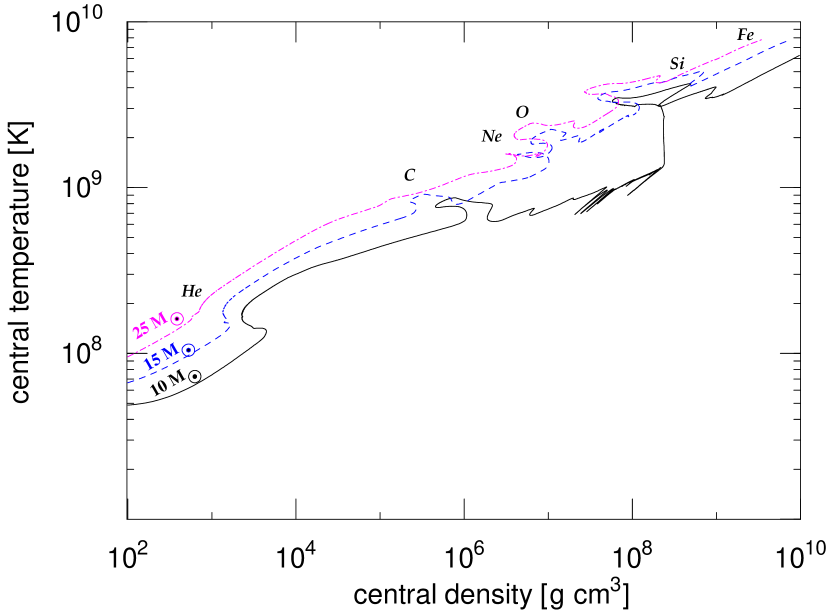
We consider here stars in the mass range of . The basic information about the physical conditions in the core of these stars can be obtained from simple considerations of hydrostatic equilibrium and balance between energy generation and loss. Assuming for the moment that the interiors of these stars can be described as ideal, nondegenerate gas, from the consideration of hydrostatic equilibrium one can find a simple relation among the mass , central temperature and central density (Clayton, 1983; Arnett, 1996):
| (4) |
where , with the mean number of electrons per baryon, and with and the mass fraction and atomic number of species respectively.
The curves in Fig. 1 represent the evolution of the central temperature and density for stars of three different masses, as found with our numerical code. Once one fuel is exhausted, the star follows a period of compression, which lasts until the temperature and density satisfy the required condition for the ignition of another nuclear reaction. We can see that these stars indeed approximately follow Eq. (4): in particular, the more massive ones have higher central temperatures. This simple fact will have important implications later.
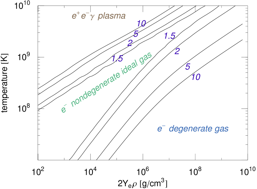
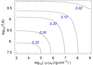
The approximation of ideal nondegenerate gas is valid for a relatively limited set of densities and temperatures, as seen in Fig. 2 which shows the ratio of the combined electron and photon pressure to the corresponding electron ideal gas pressure, . At high temperatures and low densities the pressure is dominated by radiation (photons and relativistic electron-positron plasma). At lower temperatures and high densities, the pressure is set by electron degeneracy.
Comparing Figs. 1 and 2, we see that the evolutionary trajectory of the star indeed lies almost entirely in the region where the ideal gas equation of state applies, except at the very last stages of the evolution which are on the edge of being degenerate. The lower mass stars considered in Fig. 1, having lower central temperatures, are more subject to the effects of degeneracy which set in after the start of the carbon burning (Arnett, 1996).
Two important observations need to be made at this point. First, so long as there is steady nuclear burning at the center, the star has to be outside, or at least on the edge, of the degenerate region. Indeed, a strongly degenerate system does not have the necessary negative feedback mechanism to regulate the rate of burning: energy production does not lead to expansion and cooling of the central region if the pressure is independent of temperature, as is the case for strongly degenerate systems (see, e.g., Raffelt 1996). The detour of the star through the region of high degeneracy seen in Fig. 1 indicates that the nuclear burning at this stage happens in a shell rather than in the core (Woosley et al., 2002). When the burning reaches the center, the temperature jumps and the feedback is enabled. As we will see, this behavior will be even more pronounced in the presence of the neutrino magnetic moment.
Second, there is an important physical distinction between the regimes of non-relativistic and relativistic degeneracy. The former is characterized by an adiabatic exponent (polytropic index )††\dagger††\daggerWe use the standard definition relating density and pressure . while the latter has (). A non-relativistic degenerate gas responds more strongly to compression than a relativistic one. In fact, corresponds to the edge of stability: if a sufficient fraction of the stellar core has this adiabatic exponent, the star becomes unstable to collapse (Zeldovich & Novikov, 1971). In the case of white dwarfs, this leads to the well-known upper limit on the mass, the Chandrasekhar mass. In our case of extra cooling, this will lead to the appearance of a new type of supernova.
We now turn to the mechanisms of energy loss. Energy generated by nuclear reactions is lost either through the surface of the star as photon radiation, or through the volume via neutrino emission. Photon energy loss per unit mass is about for stellar masses considered here (see, e.g., Arnett 1996, § 6.4). Neutrino cooling becomes important when the emission rate per unit mass exceeds this value.
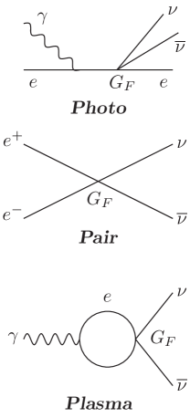
At the temperatures and densities of interest for our discussion, neutrinos are dominantly produced by the following processes (see Beaudet et al. 1967; Dicus 1972 and reference therein):
-
1.
photo process, ;
-
2.
pair process, ;
-
3.
plasma process, ,
also known as plasmon decay; -
4.
bremsstrahlung, .
The diagrams for the first three of these processes are depicted in Fig. 4.
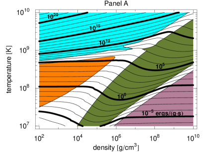
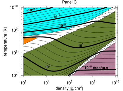
Which of these processes dominates depends on the density and temperature, as seen in Fig. 3a. The contour lines show the rate of energy loss, and are computed using the expressions for the neutrino cooling rates given in Itoh et al. (1996). These rates are used as a starting point in our numerical analyses, to compute the reference models with standard particle physics.
Superimposing Fig. 1 to Fig. 3a, we see that in the early burning stages (H- and He-burning), the neutrino production is dominated by the photo process. The energy loss (see the Eq. (A1) or contour lines in Fig. 3a), however, is still small compared to the stellar luminosity, . The neutrino energy loss starts dominating over the radiation only after central helium depletion, for temperatures above . When carbon is ignited, , the star is already losing most of its energy through neutrinos. For the more massive stars (see the curve corresponding to and in Fig. 1), neutrinos will be mainly produced by the pair process. For lower mass stars, however, there will be a competition between the pair and plasma processes. As we see the bremsstrahlung process is never important for a massive star.
Since the neutrino emission rate increases rapidly with temperature (contours lines in Fig. 3a), the fuel is consumed faster in the late stages of stellar evolution. For this reason, these later stages are characterized by progressively shorter time scales. In fact, a massive star spends about of its life burning H, and almost all of the remaining burning He. The time scale for the other burning stages is thousands of years for C, years for Ne and O, and only days for Si (Woosley et al., 2002).
In our numerical model (see details in Sect. 4), stars whose initial mass is above can ignite all burning phases (H, He, C, Ne, O, and Si burning)111For a discussion of how this threshold value varies between different codes, see (Poelarends et al., 2008). They end up with a typical “onion structure” with iron in the center and several layers around, in which fusion of lighter elements occurs. No energy can be gained by fusion reactions in the iron core, and once its mass exceeds the star collapses producing a CCSN.
Stars less massive than about have a different destiny. If the initial mass is less than about they never reach the stage of carbon-burning and end their life as carbon-oxygen white dwarfs (CO-WDs, see the bottom row of Fig. 7). If their initial mass is in the range , they do ignite carbon but not neon, and end their lives as oxygen-neon-magnesium white dwarfs (ONeMg WD). These numbers are important to us because they will be shifted by the presence of the additional cooling. Moreover, a new evolution possibility will be opened up.
We also note that the stars that we just classified as making ONeMg WDs could yet have another fate. They are close to the Chandrasekhar mass, and, after a typical “deep third dredge-up” that mixes the envelope with helium layer of the core, the core may continue to grow by hydrogen/helium shell burning. Eventually, collapse of the core may occur due to electron capture and a supernova can result (electron capture supernova, ECSN, Miyaji et al. 1980). Such a supernova typically would produce only very little . The details of whether the core can grow highly depends on the dredge-up (mixing) after and between the thermal pulses of the hydrogen/helium shell burning, competing with the mass loss of star that terminates core growth when the envelope has been lost. The historical developments on this topic are summarized in Woosley et al. (2002), while some recent developments are discussed in, e.g., Poelarends et al. (2008). Due to the uncertainty of the mass range of ECSN, we will consider them as part of our ONeMg core “bin” and just note that they comprise some fraction of the upper end of the ONeMg WD mass range.
Also note that we only consider single star evolution here. Special evolution paths that may occur in binary star systems, like, e.g., Type I SNe, are not considered in this paper.
3.2. Effects of the -induced extra cooling
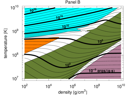
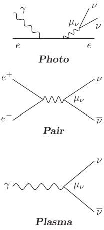
If neutrinos have a non-vanishing magnetic moment, additional processes shown in Fig. 5 must be considered. It turns out that the main effect of the neutrino magnetic moment is to increase the plasmon decay rate. For example, for , density and temperature , the non-standard plasma process energy loss is about larger than the standard one (see Eq. B1). On the other hand, for the same value of the non-standard pair production rate never exceeds of the standard one (see Fig. 9). Details of the analysis of the modified energy loss rates are provided in Appendix B.
Graphically, the effects of the magnetic moment are shown in Panels (b) and (c) of Fig. 3. We see that the plasmon dominated region enlarges considerably. Comparing Fig. 3 with Fig. 1, we see that the star “misses” the plasmon dominated region, while the and stars, having lower central temperatures, enter it. Therefore, for them the effects of the anomalous cooling should be important.
The above argument does not take into account possible feedback effects of the extra cooling on the evolutionary trajectory. Indeed, such feedback might be anticipated on general grounds: extra cooling, if sufficiently strong, can lead to the decrease of temperature which would in turn push the star deeper in the plasmon dominated degenerate region. Once the effects of degeneracy become important, cooling does not change the pressure consistently and so there is not much compressional heating as a reaction (Arnett, 1996). Thus, a qualitative change in the evolutionary trajectory might be expected.
We will now see how these qualitative expectations are borne out by the details numerical simulations.
4. Massive Stars and non-standard Cooling: Results of Numerical Modeling
4.1. Numerical modeling
Our numerical modeling is based on KEPLER, a one-dimensional implicit hydrodynamics stellar evolution code (Weaver et al., 1978). The physical ingredients of this code – such as the treatment of convection, opacities, etc – in the case of the standard physics are well documented in the literature (Woosley et al., 2002; Woosley & Heger, 2007; Heger & Woosley, 2008).
In order to simulate the effects of non-standard cooling in the evolution of massive stars, we modified the neutrino cooling routine of the code. Specifically, we computed the energy loss induced by the electromagnetic pair production (see appendix) and derived an interpolating function which is accurate at the level of in all the region of interest. The bremsstrahlung and photo processes were left unchanged since they do not play any role in our analysis.222A simulation with the bremsstrahlung and photo induced cooling doubled showed, as expected, no sensitive changes in the evolution of the star. For the plasma process we used the fitting function given in Haft et al. (1994) which is shown to be better than in all the region of interest for our purpose (see Fig. 8e of Haft et al. 1994).
We used the modified code to compute a two dimensional grid of data points, varying the mass of the star, , and the value of the neutrino magnetic moment, . The results are discussed below.
4.2. Results: Overview
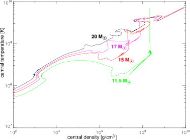
Figure 6 displays the evolution of the central temperature and density for stars of four representative masses: , , , and . These simulations include our largest extra cooling of .
As expected, we see that the evolution of the most massive of these stars, , shows no visible departure from the standard trajectory (Fig. 1). The lower mass stars, in contrast, deviate from their standard trajectories into the region of lower temperature. The curves start to bend between the He- and the C-burning stages, that is as soon as the neutrino cooling becomes more important than the radiation energy loss. The deviation becomes more pronounced the lower the mass of the star, again as anticipated.
The physics behind this phenomenon is easy to understand. As the CO core contracts following He burning, the heat that would otherwise increase the temperature to the point of carbon ignition is instead lost due to the additional cooling. The core is unable to stay on the “ideal gas” trajectory and instead collapses to a degenerate configuration. The center of core is too cold to ignite carbon burning, which is instead ignited off-center. The center becomes a relatively “cold” white dwarf () surrounded by a hotter burning shell (). Notice that while off-center ignition is observed in the standard case for lower mass stars (, see Fig. 1), here it is seen for stars of .
What happens next depends on the mass of the star. In the case of the star, the burning eventually reaches the center. At this point, the corresponding curve in Fig. 6 abruptly jumps back up to the standard “ideal gas” trajectory. The silicon burning stage in the center ensues and the star eventually undergoes iron core collapse. The remarkable detour into the degenerate region results in a somewhat different composition of the supernova progenitor (see Sect. 4.5).
A dramatically different fate awaits stars of lower mass, as represented by the curve. In this case, the detour in the degenerate region is more pronounced, with the central temperature dropping down to . The shell burning of CO extinguishes before reaching the center. As a result of the outer shell burning, the relativistic degenerate CO core builds up until it reaches the Chandrasekhar limit. The core then undergoes a thermonuclear runaway of carbon burning, consuming the CO fuel (CO explosion). This is indicated as indicated by the vertical line in the Fig. 6. In effect, the extra cooling leads to new kind of supernova – a SN Type Ia-like thermonuclear explosion inside a massive star – which perhaps could be viewed as new “Type I.7”. Our simulation stops at this point.
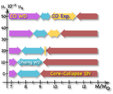
The fates of the stars of different masses as a function of the neutrino magnetic moment are shown in Fig. 7. We see that neutrino magnetic moment appreciably shifts the mass thresholds between the different outcomes. In the presence of the extra cooling, more and more massive stars are unable to ignite carbon burning. The CO window expands as a result and the ONeMg window shrinks. The CO explosion window first opens up at and for covers star with masses . A complete overview of all the models computed is given in Table 1 of Appendix C.
4.3. Changes of the WD/CCSN Thresholds
As mentioned earlier, one of the effects of the extra cooling is to make more difficult the ignition of various reactions, in particular carbon, oxygen and Neon. To burn those nuclei now requires a larger stellar mass, meaning that the threshold mass separating stars that end up as white dwarfs from those that end up as supernovae increases, as seen in Fig. 7.
This may have interesting observational implications. In particular, in recent years there has been important progress identifying progenitors of observed supernovae. Hints are accumulating that stars of initial mass do, in fact, end up as supernova explosions. A particular case is supernova SN 2003gd (Type II-P), for which the observations favor a red supergiant progenitor of mass (Van Dyk et al., 2003; Smartt et al., 2004; Van Dyk et al., 2006).
The situation with observations continues to improve at a rapid pace. For example, very recently a progenitor of supernova SN 2008bk (also a Type II-P) was identified to be a red supergiant with the mass of (Mattila et al., 2008). Likewise, a recent study of 20 progenitors of Type II-P supernovae finds that the minimum stellar mass for these stars is (Smartt et al., 2008). Referring back to Fig. 7, we see that values are already disfavored. It seems highly likely that more observational progress is to follow.
The interpretation of the observations relies, among many factors, on the stellar models used to infer the mass of the progenitor from its color and luminosity. Hence, further refinement of the stellar models would also be beneficial. To this end, it must be mentioned that the magnetic moment cooling by itself does not change the relationship between the surface characteristics and the mass: our simulation shows changes in the central region of the star at late stages of the evolution, but not in the surface characteristics.
4.4. A New Type of Supernova
The appearance of a new type of supernova as a consequence of the additional cooling is perhaps the most remarkable finding of our simulations. Should such objects have distinct characteristics not observed in actual supernova explosions, a robust bound on the magnetic moment, , would result.
We again stress that we were unable to follow the development of the explosion beyond the ignition of the degenerate CO burning. Such calculations would be highly desirable. Provisionally, we could consider a plausible model of a Type Ia supernova exploding inside a red supergiant. A simple estimate we performed shows that, especially for stars in the low mass end of the “CO explosions” bin, the amount of energy available upon burning of the entire CO core is enough to disrupt the star, though a detailed hydrodynamic study to confirm this assessment has yet to be performed. The resulting explosion would leave no neutron star remnant, and no neutrino signal would be observed. The amount of 56Ni and 56Co could be close to what is produced in a Type Ia explosion, (Blinnikov et al., 2006). This would significantly exceed the amounts ejected in a standard core collapse explosion, , or in possible ECSNe from our ONeMg WD bin. As discussed by Woosley et al. (2002), the decay of 56Co to 56Fe (half-life 77 days) is observationally very significant, giving a “radioactive tail” to the light curve. Thus, excessive amounts of 56Co could be seen. For the current accuracy of the determination of 56Ni mass from observations see, e.g., Fig. 9 in Smartt et al. (2008).
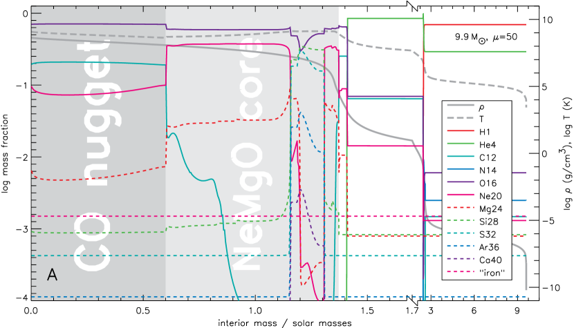
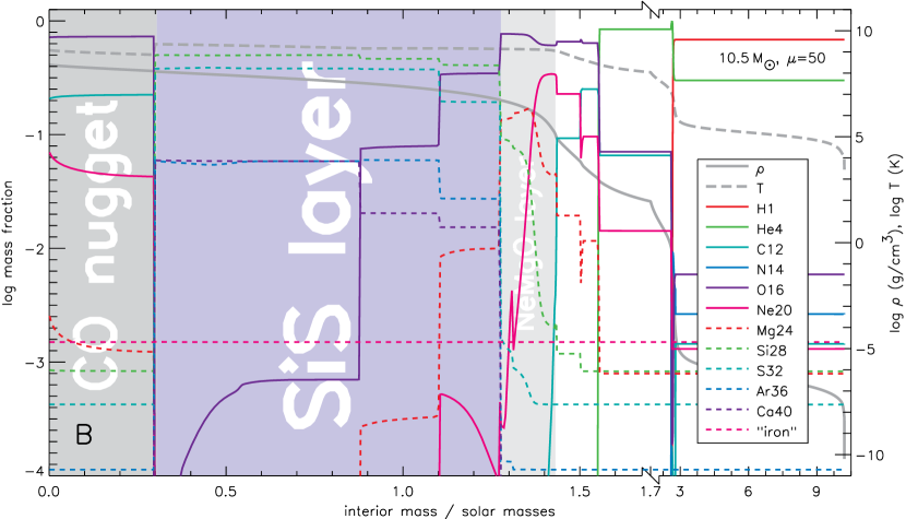
Notice that in the previous argument we concentrated on the low-mass end of the “CO explosions” bin. In fact, the pre-explosion composition of the stars in the “CO explosions” bin varies with the mass of the star. Two typical examples are shown in Fig. 8. We see that only the inner fraction of the core has a CO composition. This CO inner core is surrounded by either a ONeMg layer at lower masses, or a silicon-sulfur (SiS) layer (from ONeMg shell burning) at higher masses. We find that the size of the central CO “nugget” decreases as the mass of the star increases. This will affect densities, nucleosynthesis, and energetics of the explosion.
At the upper mass limit of the “CO explosions” bin, the energy may eventually become insufficient to disrupt the star; in this case, a burning pulse may eject the outer layer just before the final core collapse SN, making it rather bright at the peak due to the interaction of the core collapse SN ejecta and the previously ejected layers. This mechanism is similar to the model for pair-instability supernovae presented in Woosley et al. (2007). The resulting SN would have little to power the tail of the light curve.
In a few cases at the upper mass limit we also observe the formation of an “iron” layer from silicon shell burning; these cases have only a tiny () CO core left in the center and collapse as core collapse SNe before igniting the central CO nugget; they would probably be indistinguishable from regular CCSNe.
The detailed information from our simulations is collected in Table 1. We can see that a significant fraction of the supernovae in the “CO explosions” bin do have sizable CO cores, enough to disrupt the stars and give the characteristic excess 56Co observational signature.
Lastly, we note recent observations of the Kepler’s supernova remnant (Reynolds et al., 2007)333We thank Carles Badenes for bringing this interesting study to our attention.. The abundance of iron in the shocked ejecta together with no evidence for oxygen-rich ejecta indicate that this object underwent a thermonuclear explosion. Curiously, a detailed analysis described in that paper suggests the possibility of a Type Ia explosion in a more massive progenitor. That the explosion occurred in the environment that is not low in metallicity is especially interesting. Clearly, further observational studies are very desirable.
4.5. Other Effects
There are several other effects of the extra cooling that are worth mentioning. For example, the resulting composition of the core-collapse supernova progenitor is somewhat modified. Our calculations of the star show the size of the CO core decreases by with . This small change could be of interest, since the explosion mechanism is a sensitive function of the chemical composition.
Another effect is the change of the presupernova neutrino signal (Odrzywolek et al., 2004). This occurs because the last stage before the iron core collapse – Si burning – proceeds significantly faster since the energy escapes the core more easily. For and , the Si shell burning time is only about 8 hours, instead of 15 hours for . The pre-supernova neutrino signal at a future megaton-sized neutrino detector could be shorter with higher luminosity.
Other effects may be revealed upon a more detailed investigation. For example, the extra cooling would modify the nucleosynthetic yields of various elements.
5. Conclusion and Perspectives
For certain kinds of new physics, useful astrophysical constraints can be obtained using simple order-of-magnitude analytical estimates. Examples are provided by various theories with extra dimensions (see, e.g., Cullen & Perelstein 1999; Hannestad & Raffelt 2002; Friedland & Giannotti 2008). In contrast, the treatment of the problem given here requires a detailed analysis with a sophisticated stellar evolution code.
As we have seen, stars with masses in the range are indeed sensitive to the neutrino magnetic moment. The additional cooling it introduces does not simply change the evolutionary time scales of these stars, but leads to the appearance of qualitatively new features in the evolution. The physics involved is very rich and more detailed investigations of many aspects are clearly desirable. We have undertaken here the first step to explore the subject. Let us now summarize our main results and consider some perspectives.
1) We have shown that the magnetic moment of the size , which is below the experimental bound, would modify the evolution of stars with the masses . The evolution of heavier stars is unchanged. This is a consequence of the fact that heavier stars have higher central temperatures and as a result “miss” the region of the parameter space where the extra cooling operates.
2) The minimal value of to which the star is sensitive depends on the initial mass. For stars whose initial mass is about , this value is as low as . The sensitivity of massive stars to the neutrino magnetic moment is thus comparable to that of the HB stars (Raffelt et al., 1989). Notice that Raffelt (1990) found that the analysis of RG cooling yields a more stringent bound, .
3) The extra cooling due to the neutrino magnetic moment shifts the threshold masses for the different final stages of the evolution. The number of carbon-oxygen white dwarfs increases, while the corresponding number of the oxygen-neon-magnesium white dwarfs and core collapse supernovae decreases. These shifts are graphically illustrated in Fig 7. This effect could be constrained using observations of supernova progenitors. Such data is now coming in at a rapid pace.
4) According to our code, stars with initial mass undergo a thermonuclear explosion for values of larger than . This is a new feature, absent in the standard model evolution, and in principle observable. The initial mass region for which this happens enlarges with larger , and is depicted in Fig. 7, labeled as “CO explosion”. For we predict that roughly one in five of the stars which do not become WDs end their lives with this thermonuclear explosion, whereas the others become CCSNe.
5) The final composition of the presupernova is a function of . This might be of interest since the explosion mechanism is a sensitive function of the chemical composition.
6) For stars that end their lives as CCSNe, a possible presupernova neutrino signal at a future megaton water Cherenkov neutrino detector would be modified in the presence of the additional cooling. The neutrino flux would be higher and the duration shorter.
7) Our conclusions are based on a numerical simulation performed with the KEPLER code. A reliable prediction of the threshold masses between different kinds of WDs and CCSN depends on, among other ingredients, the treatment of convection, which varies between the codes. A comparison of different codes (standard evolution only) was performed by Poelarends et al. (2008), yielding slightly different predictions of the thresholds. In the case of nonstandard physics, a similar comparison would be very useful. Additionally, one has to keep in mind other uncertainties that affect stellar evolution, such as the initial stellar composition (e.g., Tur et al. 2007) and the natural distribution of stellar rotation rates (e.g., Heger et al. 2000).
8) Beyond this list, various other aspects of the extra cooling could be considered, such as the changes in the nucleosynthesis of various elements.
Appendix A APPENDIX A: Energy loss due to standard neutrino interactions
In this appendix we give approximate expressions for the standard neutrino cooling rates as a function of density and temperature, in order to give an analytical description of Fig. 3a. We restrict ourselves only to the regions relevant to the evolution of massive stars.
At temperatures below and low densities (orange region in the middle left in Fig. 3a) the photo process dominates. Energy loss per unit mass due to this process is roughly (Petrosian et al., 1967)
| (A1) |
where . At higher temperatures (top turquoise region in Fig. 3a) pair production instead dominates. The energy loss is roughly(Fowler & Hoyle, 1964)
| (A2) |
for and
| (A3) |
for , where and .
Both the above equations apply only for non-degenerate plasma. When degeneracy becomes important the pair emission is exponentially suppressed by the electron chemical potential. In this regime, the main loss mechanism is the neutrino emission via plasmon decay (green region in the middle of Fig. 3a). This rate was first calculated by Inman & Ruderman (1964). For densities such that , the energy loss due to this process is approximately
| (A4) |
At very high densities (), this emission is exponentially suppressed by the plasma frequency and the bremsstrahlung process becomes the dominant one.
Appendix B APPENDIX B: Energy loss due to non-standard neutrino interactions
If neutrinos have a non-vanishing magnetic moment, the production mechanisms (pair, plasma, photon, bremsstrahlung) would receive an additional electromagnetic contribution from the interaction term of Eq.(1), as shown in Fig. 5. We restrict ourselves only to the processes relevant for the evolution of massive stars, namely plasma and pair production (the photo process dominates neutrino energy loss in a region where the star cools mainly via radiative energy loss).
B.1. Plasma processes
The standard and electromagnetically induced plasmon emission rates ( and ) depend differently on the plasma frequency, and hence on the density. This behavior can be anticipated on the grounds of dimensional analysis. The energy loss rate can be schematically written as . Therefore the ratio of the standard and the additional nonstandard cooling rates is equal to the corresponding ratio of the plasmon decay rates, (cf. Friedland & Giannotti 2008). The latter, in turn, can be estimated by dimensional analysis. The rates are proportional to the squares of the corresponding coupling constants, or . The remaining dimension should be fixed by alone. (In the rest frame of the plasmon, cannot enter.) Therefore, . In the region of temperature and density of interest for us, a detailed calculation gives (Haft et al., 1994)
| (B1) |
where the plasma frequency is numerically given by, e.g., Raffelt (1996),
| (B2) |
with in . Therefore at low densities, , the ratio between the electromagnetic induced plasmon emission rate and the standard one is inversely proportional to the density, whereas at high density , it is inversely proportional to . Finally, taking for example , equation (B1) shows that, for density sufficiently low, the non-standard plasma process can be much larger than the standard one. Therefore, when the non-standard neutrino interactions are turned on, the region where the plasma process is dominant becomes larger, especially at low densities (see panel (b) and (c) of Fig. 3).
B.2. Pair production
The energy loss per unit time and volume in neutrino pair production is given by the transition probability for annihilation multiplied by the neutrino pair energy and integrated over the density of both initial and final states. This reads
| (B3) |
where is the chemical potential, is the electron-positron relative velocity and represents the spin averaged cross-section for annihilation. The quantity is Lorentz invariant and is given by (, )
| (B4) |
in terms of the spin-averaged squared invariant amplitude . If the pair production proceeds via neutrino magnetic moment, we find (, , )
| (B5) |
where represents the effective dipole moment:
| (B6) |
Integrating over the invariant phase space leads to
| (B7) |
or equivalently . Performing the angular integrations in Eq. B4 we then find
| (B8) |
showing that the expression for the luminosity factorizes in the product of two one-dimensional integrals.
Following Beaudet et al. (1967), we now define the dimensionless variables
| (B9) |
and the dimensionless integrals
| (B10) |
The luminosity due to non-standard pair production reads
| (B11) |
and is a function of the temperature and the chemical potential. In order to have a function of temperature and density, the chemical potential must be solved in terms of temperature and density. This requires the solution of the following equation(Beaudet et al., 1967)
| (B12) |
which cannot in general be inverted analytically in terms of . The numerical solutions are plotted in Fig. 1 of Beaudet et al. (1967).
In order to assess the impact of non-standard cooling, the above result has to be compared to the Standard Model emission rate (Dicus, 1972):
| (B13) | |||||
Here and , with the weak mixing angle numerically given by . The energy loss due to and is obtained form by replacing and .
A simple comparison of the standard and non-standard pair production amplitudes suggests that the two contributions are of comparable size if . Using the full expressions of Eqs. B11 and B13 we plot in Fig. 9 the ratio for in the region of interest in the plane. The results show that indeed the non-standard loss never exceeds of the electro-weak one, being most important in the non-relativistic and non-degenerate region. From the behavior of in the relativistic and/or degenerate limit one can simply verify that in these physical regimes, as shown in Fig. 9.
For the numerical implementation in the stellar evolution code we have used the simple fitting formula
| (B14) | |||||
| (B15) | |||||
| (B16) | |||||
| (B17) |
where is defied by , , and . The fitting formula is accurate at the level of or better in the region defined by and .
Finally, in the region where the pair process dominates neutrino emission, the additional energy loss per unit time and mass is approximately given by:
| (B18) |
where . Comparing with Eqs. (A2) and (A3) we see that this energy loss is never more that of the standard model value, if is below the experimental bound.
Appendix C APPENDIX C: Detailed Listing of Model Results
Table 1 summarizes our calculations and results for different values of .
| Comment | |
| AGB, CO WD | |
| AGB, CO WD with NeMgO outer layer, CO center | |
| AGB, ONeMg WD, 3rd dredge-up, vast C shell burning, CO core left in center | |
| AGB, OMeMg WD, 3rd dredge-up | |
| 3rd dredge-up, may make ECSN | |
| NeO thermonuclear runaway, weak explosion; fallback could still be possible | |
| CCSN, ONeMg core, explosive ignition inside Fe shell | |
| CCSN | |
| AGB, CO WD | |
| AGB, ONeMg WD, 3rd dredge-up, vast C shell burning, up to CO core left in center | |
| AGB, ONeMg WD (3rd dredge-up) | |
| ONeMg WD or ECSN | |
| CCSN, ONeMg core with SI Shell burning, | |
| CCSN, central NeO ignition, weak explosion, fallback of Fe core | |
| CCSN | |
| AGB, CO WD | |
| AGB, ONeMg WD | |
| O/Ne/C thermonuclear runaway | |
| SiS core ( O), CCSN | |
| Si explosion, 3rd dredge-up of He shell, CCSN | |
| CCSN, Si detonation | |
| CCSN | |
| CCSN, SiS nugget at center, should make Si detonation | |
| CCSN | |
| AGB, CO WD | |
| AGB, CO WD with ONeMg layer | |
| AGB, ONeMg WD with C in center | |
| AGB, ONeMg, C in center, deep 3rd dredge-up | |
| C thermonuclear runaway, CO nugget, inside ONeMg core | |
| C thermonuclear runaway, CO nugget in center | |
| CCSN | |
| AGB, CO WD, He left close to center | |
| AGB, CO WD | |
| AGB, CO WD, starting and increasing C shell burning | |
| AGB, CO WD, layer with Ne C | |
| AGB, ONeMg WD, CO core | |
| AGB, ONeMg WD, CO core, no 3rd dredge-up | |
| C thermonuclear runaway, CO core, He core, 3rd dredge-up, NeO shell | |
| C thermonuclear runaway, CO core, He core, NeO shell | |
| C thermonuclear runaway, CO core, He core, SiS shell | |
| C thermonuclear runaway, CO core, He core, Fe shell CCSN | |
| C thermonuclear runaway, CO core, He core, SiS shell | |
| C thermonuclear runaway, CO core, He core, Fe shell CCSN | |
| C thermonuclear runaway, CO core, He core, SiS shell | |
| C thermonuclear runaway, CO core, He core, NeO shell | |
| C thermonuclear runaway, CO core, He core, SiS shell | |
| CCSN | |
References
- Arnett (1996) Arnett, D. 1996, Princeton series in astrophysics, Princeton, NJ: Princeton University Press, —c1996,
- Ayala et al. (1999) Ayala, A., D’olivo, J. C., & Torres, M. 1999, Phys. Rev. D, 59, 111901
- Babu & Mohapatra (1990) Babu, K. S., & Mohapatra, R. N. 1990, Physical Review Letters, 64, 1705
- Barbieri & Mohapatra (1988) Barbieri, R., & Mohapatra, R. N. 1988, Physical Review Letters, 61, 27
- Barbieri & G. Fiorentini (1988) Barbieri, R. & Fiorentini, G 1988, Nucl. Phys. B, 304, 909
- Barbieri & Mohapatra (1989) Barbieri, R., & Mohapatra, R. N. 1989, Physics Letters B, 218, 225
- Barr et al. (1990) Barr, S. M., Freire, E. M., & Zee, A. 1990, Physical Review Letters, 65, 2626
- Beaudet et al. (1967) Beaudet, G., Petrosian, V., & Salpeter, E. E. 1967, ApJ, 150, 979
- Beda et al. (2007) Beda, A. G., Brudanin, V. B., Demidova, E. V., Egorov, V. G., Gavrilov, M. G., Shirchenko, M. V., Starostin, A. S., & Vylov, T. 2007, ArXiv e-prints, 705, arXiv:0705.4576
- Bell et al. (2005) Bell N. F., Cirigliano V., Ramsey-Musolf M. J., Vogel P., & Wise M. B. 2005, Physical Review Letters, 95, 151802
- Bell et al. (2006) Bell N. F., Gorchtein M., Ramsey-Musolf M. J., Vogel P., & Wang P. 2006, Physics Letters B, 642, 377
- Bernstein et al. (1963) Bernstein J., Ruderman M., & Feinberg G. 1963, Physical Review, 132, 1227
- Blinnikov & Dunina-Barkovskaya (1994) Blinnikov, S. I., & Dunina-Barkovskaya, N. V. 1994, MNRAS, 266, 289. The original idea of considering white dwarfs to probe the neutrino electromagnetic properties is found in Sutherland, P., Ng, J. N., Flowers, E., Ruderman, M., & Inman, C. 1976, Phys. Rev. D, 13, 2700
- Blinnikov et al. (2006) Blinnikov, S. I., Röpke, F. K., Sorokina, E. I., Gieseler, M., Reinecke, M., Travaglio, C., Hillebrandt, W., & Stritzinger, M. 2006, A&A, 453, 229
- Castellani & degl’Innocenti (1993) Castellani, V., & degl’Innocenti, S. 1993, ApJ, 402, 574
- Catelan et al. (1996) Catelan, M., de Freitas Pacheco, J. A., & Horvath, J. E. 1996, ApJ, 461, 231
- Clayton (1983) Clayton, D. D. 1983, Chicago: University of Chicago Press, 1983
- Cowan & Reines (1957) Cowan, C. L., & Reines F. 1957, Physical Review, 107, 528
- Cullen & Perelstein (1999) Cullen, S., & Perelstein, M. 1999, Physical Review Letters, 83, 268
- Davidson et al. (2005) Davidson S., Gorbahn M., & Santamaria A. 2005, Physics Letters B, 626, 151
- Daraktchieva et al. (2005) Daraktchieva Z., et al. [MUNU Collaboration] 2005, Physics Letters B, 615, 153
- Dicus (1972) Dicus, D. A. 1972, Phys. Rev. D, 6, 941
- Dolgov (2002) Dolgov, A. D. 2002, Phys. Rep., 370, 333
- Fowler & Hoyle (1964) Fowler, W. A., & Hoyle, F. 1964, ApJS, 9, 201
- Friedland (2005) Friedland, A. 2005, ArXiv High Energy Physics - Phenomenology e-prints, arXiv:hep-ph/0505165.
- Friedland & Giannotti (2008) Friedland, A., & Giannotti, M. 2008, Physical Review Letters, 100, 031602
- Fujikawa & Shrock (1980) Fujikawa, K., & Shrock, R. E. 1980, Physical Review Letters, 45, 963
-
Galbiati (2008)
Galbiati, C., talk at the XXIII
International Conference on Neutrino Physics and Astrophysics
(Neutrino 08);
http://www2.phys.canterbury.ac.nz/~jaa53/prel_programme.htm - Georgi & Randall (1990) Georgi, H., & Randall, L. 1990, Physics Letters B, 244, 196
- Grimus & Neufeld (1991) Grimus W., & Neufeld H. 1991, Nucl. Phys. B, 351, 115
- Haft et al. (1994) Haft, M., Raffelt, G., & Weiss, A. 1994, ApJ, 425, 222
- Hannestad & Raffelt (2002) Hannestad, S., & Raffelt, G. G. 2002, Physical Review Letters, 88, 071301
- Heger et al. (2000) Heger, A., Langer, N., Woosley, S. E. 2000, ApJ, 528, 368.
- Heger & Woosley (2008) Heger, A., & Woosley, S. E. 2008, ArXiv e-prints, 803, arXiv:0803.3161
- Inman & Ruderman (1964) Inman, C. L., & Ruderman, M. A. 1964, ApJ, 140, 1025
- Itoh et al. (1996) Itoh, N., Hayashi, H., Nishikawa, A., & Kohyama, Y. 1996, ApJS, 102, 411
- Iwamoto et al. (1995) Iwamoto, N., Qin, L., Fukugita, M., & Tsuruta, S. 1995, Phys. Rev. D, 51, 348
- Lattimer & Cooperstein (1988) Lattimer, J. M., & Cooperstein, J. 1988, Physical Review Letters, 61, 23
- Lee & Shrock (1977) Lee, B. W., & Shrock, R. E. 1977, Phys. Rev. D, 16, 1444
- Marciano & Sanda (1977) Marciano, W. J., & Sanda, A. I. 1977, Physics Letters B, 67, 303
- Mattila et al. (2008) Mattila, S., Smartt, S. J., Eldridge, J. J., Maund, J. R., Crockett, R. M., & Danziger, I. J. 2008, ArXiv e-prints, 809, arXiv:0809.0206
- Miranda et al. (2004) Miranda, O. G., Rashba, T. I., Rez, A. I., & Valle, J. W. 2004, Physical Review Letters, 93, 051304
- Miyaji et al. (1980) Miyaji, S., Nomoto, K., Yokoi, K., & Sugimoto, D. 1980, PASJ, 32, 303
- Nötzold (1988) Nötzold, D. 1988, Phys. Rev. D, 38, 1658
- Odrzywolek et al. (2004) Odrzywolek, A., Misiaszek, M., & Kutschera, M. 2004, Astroparticle Physics, 21, 303
- Petrosian et al. (1967) Petrosian, V., Beaudet, G., & Salpeter, E. E. 1967, Physical Review 154, 1445
- Poelarends et al. (2008) Poelarends, A. J. T., Herwig, F., Langer, N., & Heger, A. 2008, ApJ, 675, 614; arXiv:0705.4643
- Raffelt et al. (1989) Raffelt, G., Dearborn, D., & Silk, J. 1989, ApJ, 336, 61
- Raffelt (1990) Raffelt, G. G. 1990, ApJ, 365, 559 ; Raffelt, G. G. 1990, Physical Review Letters, 64, 2856
- Raffelt & Weiss (1992) Raffelt, G., & Weiss, A. 1992, A&A, 264, 536
- Raffelt (1996) Raffelt, G. G. 1996, Stars as laboratories for fundamental physics: the astrophysics of neutrinos, axions, and other weakly interacting particles / Georg G. Raffelt. Chicago : University of Chicago Press, 1996.
- Raffelt (1999) Raffelt, G. G. 1999, Phys. Rep., 320, 319
- Raffelt (2000) Raffelt, G. G. 2000, Phys. Rep., 333, 593
- Reynolds et al. (2007) Reynolds, S. P., Borkowski, K. J., Hwang, U., Hughes, J. P., Badenes, C., Laming, J. M., & Blondin, J. M. 2007, ApJ, 668, L135
- Smartt et al. (2004) Smartt, S. J., Maund, J. R., Hendry, M. A., Tout, C. A., Gilmore, G. F., Mattila, S., & Benn, C. R. 2004, Science, 303, 499
- Smartt et al. (2008) Smartt, S. J., Eldridge, J. J., Crockett, R. M., & Maund, J. R. 2008, ArXiv e-prints, 809, arXiv:0809.0403
- Tur et al. (2007) Tur, C., Heger, A., and Asutin, S. M. 2007, ApJ, 671, 821.
- Van Dyk et al. (2003) Van Dyk, S. D., Li, W., & Filippenko, A. V. 2003, PASP, 115, 1289
- Van Dyk et al. (2006) Van Dyk, S. D., Li, W., & Filippenko, A. V. 2006, PASP, 118, 351
- Voloshin (1988) Voloshin M. B. 1988, Sov. J. Nucl. Phys., 48, 512
- Weaver et al. (1978) Weaver, T. A., Zimmerman, G. B., & Woosley, S. E. 1978, ApJ, 225, 1021
- Woosley et al. (2007) Woosley, S. E., Blinnikov, S.; Heger, A. 2007 Nature, 450, 390.
- Woosley et al. (2002) Woosley, S. E., Heger, A., & Weaver, T. A. 2002, Reviews of Modern Physics, 74, 1015
- Woosley & Heger (2007) Woosley, S. E., & Heger, A. 2007, Phys. Rep., 442, 269
- Zeldovich & Novikov (1971) Zeldovich, Ya. B. & Novikov, I. D. 1971, Stars and Relativity, University of Chicago Press