Extrasolar planets and brown dwarfs around A–F type stars

Abstract

Aims. Systematic surveys to search for exoplanets have been mostly dedicated to solar-type stars sofar. We developed in 2004 a method to extend such searches to earlier A–F type dwarfs and started spectroscopic surveys to search for planets and quantify the detection limit achievable when taking into account the stars properties (Spectral Type, $v\sin{i}$) and their actual levels of intrinsic variations. We give here the first results of our southern survey with HARPS.

Methods. We observed 185 A–F ($B-V$ in the range [$-$0.1; 0.6]) stars with HARPS and analysed them with our dedicated software. We use several criteria to probe different origins for the radial-velocity variations – stellar activity (spots, pulsations) or companions: bisector shape, radial-velocity variations amplitudes and timescales.

Results. 1) 64 $\%$ of the 170 stars with enough data points are found to be variable. 20 are found to be binaries or candidate binaries (with stars or brown dwarfs). More than 80 $\%$ or the latest type stars (once binaries are removed) are intrinsically variable at a 2 m s^-1precision level. Stars with earlier spectral type ($B-V$ $\leq$ 0.2) are either variable or associated to levels of uncertainties comparable to the RV rms observed on variable stars of same $B-V$. 2) We have detected one long-period planetary system (presented in another paper) around an F6IV–V star. 3) We have quantified the jitter due to stellar activity and we show that taking into account this jitter in addition to the stellar parameters (spectral type, $v\sin{i}$), it is still possible to detect planets with HARPS with periods of 3 days (resp. 10 days and 100 days) on 91 $\%$ (resp. 83 $\%$, 61 $\%$) of them. We show that even the earliest spectral type stars are accessible to this type of search! , provided they have a low projected rotational velocity and low levels of activity. 4) Taking into account the present data, we compute the actually achieved detection limits for 107 targets and discuss the limits as a function of $B-V$. Given the data at hand, our survey is sensitive to short-period (few days) planets and to longer ones (100 days) at a lower extent (latest type stars). We derive first constrains on the presence of planets around A–F stars for these ranges of periods.

1 Introduction

Since the discovery of the first exoplanet around a solar-like star in 1995, more than 250 planets have been found by radial-velocity (RV) surveys (Jean Schneider, http://exoplanet.eu). These surveys have generally focused on late-type stars (later than F8). However, knowing about the presence of planets or brown dwarfs (hereafter BDs) around more massive objects is mandatory if one wishes to investigate the impact of the mass of the central stars on the planetary formation and evolution processes.

There are theoretical indications that the mass of the planets increases with the mass of the parent star, at least for low mass stars (Ida & Lin (2005)) and that the frequency of giant planets increases linearly with the parent star mass for stars between 0.4 and 3 M_☉ (Kennedy & Kenyon (2008)), with e.g., 6 $\%$ frequency of giant planets around 1 M_☉ and 10 $\%$ frequency around 1.5 M_☉. More numerous and massive planets are consistent with what we could expect from a disk surface density increasing with stellar mass. On the other hand the shorter lifetimes of the systems as well as the lack of solid material close to the star could reduce the number of planets. Clearly, several parameters probably impact the occurence and properties of planets around massive stars, and they have not yet been fully explored.

The data to test the models are still quite limited as the largest and earliest, now long-lasting surveys had focused on solar type, main-sequence (MS) stars. In recent years, some efforts have been made nevertheless to search for planets around stars with various masses: less massive, M-type stars on the one hand, and more massive stars on the other hand. The search for planets around M stars seems sofar to confirm the previously mentionned expectations from theoretical works (see e.g., Bonfils et al. (2005); Butler et al. (2006)). As far as massive stars are concerned, the available observations are still very limited. Massive MS stars have been removed from early surveys as it was generally thought that their spectra (few lines, usually broadened by stellar rotation) would not allow planet detection and indeed, the classical RV measurements technics (based on the cross correlation of the actual spectra with a binary spectral mask corresponding to a star with an appropriate spectral type and $v\sin{i}$ = 0 km s^-1) fail to measure the RV of these stars. This lead some groups to study instead “retired” early-type, either low-mass ($\leq$ 1.6 M_☉) giants, intermediate-mass (1.6–2 M_☉) subgiants or clump giants (1.7–3.9 M_☉) (see e.g., Hatzes (2005); Niedzielski et al. (2007); Johnson et al. (2006); Johnson et al. (2007); Lovis and Mayor (2007); Sato et al. (2008)). These stars indeed have cooled out and also rotate more slowly due to coupling of stellar winds and magnetic fields; they therefore exhibit more numerous, narrower lines, which is adequate for classical RV measurements technics, and their level of activity (jitter) is relatively low (10–20 m s^-1; Hekker et al. (2006)) for giants and 10 m s^-1 for subgiants (Johnson et al. (2007) and ref. therein; Sato et al. (2008)). The data available today are still limited compared to those available on solar-type stars and less than 20 planets have been found sofar in total around these evolved stars. So far, the planets found around K subgiants stars with M $\geq$ 1.5 M_☉ are located at distances larger than 0.8 AU (Johnson et al. (2007)); this led these authors to conclude that close-in planets are rare, in agreement with some theoretical predictions on disks depletion timescales (Burkert and Ida (2007)). However, the impact of the post MS evolution of the stars on closer-in planets has not been explored yet for these stars. Concerning giant stars, all planets found so far have relatively long periods, the closest ones beeing reported at less than 0.7 AU from 2 giants, in addition to a previously reported planet at 0.7 AU by Sato et al. (2003). Numerical simulations by the same authors suggest that planets with orbits inside 0.5–1 AU around 2–3 M_☉ stars could be engulfed by the central stars at the tip of RGB due to tidal torque from the central stars. According to them, if one assumes then that most of the clump giants are post RGB stars, there is then a risk that closer planets, if present before had disappeared since the star evolved. In summary, eventhough there are some hints that hot Jupiters are not present around retired stars, it is recognized that data are still needed to definitely confirm this point. Also, as stellar evolutionary processes may have impacted the presence of planets close to the stars, it is acknowledged that data are needed on A–F MS stars (see eg Burkert and Ida (2007); see also Li, Lin and Liu (2008)). We note finally that short-period planets have indeed been found around F5–F6 MS stars through transit observations (see http://exoplanet.eu).

We developed a few years ago a dedicated software to extract the RV data around early type MS stars. The method consists in correlating, in the Fourier space, each spectrum and a reference spectrum built by summing-up all the available spectra for this star. We had shown earlier that with this approach, and taking into account the stars $B-V$ and projected rotational velocities, it is possible to find planets around A–F type stars (Galland et al. 2005a ). However, the price to pay is that more measurements are needed to find planets around A and early F dwarfs than for late F and G–K dwarfs, because of the relatively higher uncertainties in the RV measurements due to higher $v\sin{i}$ and higher effective temperature, and also because of the possible presence of pulsations or spots in the case of late F stars, the impact of which has not been quantified so far. (Note that spots or pulsations become also a limiting factor in the case of later-type stars, as well as pulsations, if one looks for low mass planets.) We started then systematic searches for low-mass companions to A–F type stars, with HARPS in the southern hemisphere and with ELODIE and then SOPHIE at OHP in the northern hemisphere. We found so far a 9.1 M_Jup (minimum mass) planet orbiting ($a$ = 1.1 AU) an F6V star, with $v\sin{i}$ = 12 km s^-1 (Galland et al. 2005b ). Very promisingly, we also detected a 21 M_Jup brown dwarf orbiting ($a$ = 0.2 AU) a pulsating A9V star with $v\sin{i}$ = 50 km s^-1 (Galland et al. (2006)); noticeably, in that case, we could disentangle stellar pulsations from the presence of a low-mass companion.

In parallel, we developed detailed simulations of stellar activity (spots) in order to estimate more quantitatively than what was available so far (Saar & Donahue (1997); Hatzes (2002)) the impact of such stellar activity on RV data and other observables (bisectors, bisectors velocity-span, photometry). We have showed that if the star $v\sin{i}$ is smaller than the spectrograph spectral resolution, depending on their location with respect to line of sight, depending also on their size, spots with realistic sizes can produce RV variations and bisector velocity-span variations quite similar to those of low mass planets. Hence, low amplitude (level of typically 20 m s^-1 or less) planetary-like RV and bisector velocity span variations cannot alone definitely prove the presence of planets around low $v\sin{i}$ G–K stars (Desort et al. (2007)) and additional criteria are mandatory to rule out spots: photometry, activity evaluation down to levels relevent to explain the amplitude of RV variations, precise knowledge of the star rotaional period, etc. The situation in that respect is much more favorable in the case of earlier-type stars as they rotate statistically faster and hence the bisector criteria can apply.

The present paper is devoted to our southern hemisphere survey. The sample, observations, measurements and diagnostics are provided in Sect. 2. The results concerning the stellar variability as well as the quantitative impact on planet detectability around the early-type stars are presented in Sect. 3. Finally we give and discuss in Sect. 4 the detection limits obtained in the present survey.

2 Sample, observations and measurements

2.1 Sample

Our HARPS sample is limited to B8 to F7 dwarfs. The limit in spectral type (ST) at F7 is set because the surveys using masking technique generally start with stars with ST later than F8. The limit at B8 is set by the precision that can be obtained with our method on stars given their ST and their $v\sin{i}$ (Galland et al. 2005a ): the detection limit of stars with ST earlier than B8 does not fall into the planet domain. Our survey is also volume-limited with an upper limit at 67 pc for the B8–A9 dwarfs and at 33 pc for the F0–F7 dwarfs. The distance was taken from Hipparcos catalogue, and stars with distance uncertainties larger than 20 $\%$ were removed. The difference in distance for both spectral types comes from the fact that we wanted to have roughly the same number of A and F stars. The dwarf nature was selected by selecting stars with absolute magnitudes within 2.5 magnitude from the Main Sequence.

Spectroscopic binaries as well as close visual binaries with separations smaller than 5″ known at the begining of the survey from Coravel or Hipparcos data were removed. Confirmed $\delta$ Scuti (from Rodriguez et al. (2000)) and $\gamma$ Doradus type stars (from Mathias et al. (2004) and http://astro.univie.ac.at/dsn/gerald/gdorlist.html) were also removed as they are known to produce RV variations over hours to a few days periods due to pulsations. Finally we removed as well Ap and Am stars, which present spectral anomalies and are often associated to binary systems. This removes a number of late A - early F type stars, crossing the $\delta$ Scuti and $\gamma$ Doradus instability strip. We ended up with 207 stars with ST between B8 and F7, and $B-V$ ranging respectively between $-$0.1 and 0.58, corresponding to mass ranging between 1.3 and 3.5 M_☉. Note that we have a relatively smaller number of stars in the [0.2; 0.4] $B-V$ range (i.e., roughly, between 1.8 and 1.4 M_☉) as we removed the known $\delta$ Scuti and $\gamma$ Doradus stars).

2.2 Observations

185 stars have been observed between August 2005 and January 2008. Figure 1 shows their position in the HR diagram. It can be seen that our survey fills a domain of the HR diagram that was not covered yet.

We usually recorded 2 consecutive high resolution ($R\simeq 115000$) spectra each time we pointed to the star (each pointing is hereafter refered to as one epoch). The spectra cover a wavelength range between 3800 and 6900 $\AA$. As far as possible we moreover tried for a given object to record data at two or three different times during one night, in order to identify possible high-frequency RV variations. We also tried whenever possible to record data on two or three consecutive nights. The time baseline for a given star varies between 5 days and more than 800 days. Only a few (11) stars have been observed during one night only, but for 15 stars we got only 4 good quality (i.e., with an absorption smaller than 2) spectra or less. We ended up with 170 dwarfs for which we recorded 6 or more good quality spectra. 45 have $B-V$ $\leq$ 0.1; 72 have $B-V$ between 0.1 and 0.4 and 53 have $B-V$ $\geq$ 0.4. We will restrain hereafter our study to those stars.

Typical exposure times ranged between 30 s and 15 min depending on the star magnitude and on the atmospheric conditions.

Table LABEL:sample provides the 170 targets observed, together with a number of relevent information on the stars (ST, $v\sin{i}$, $B-V$) and on the data obtained as well as various measurements (see below).

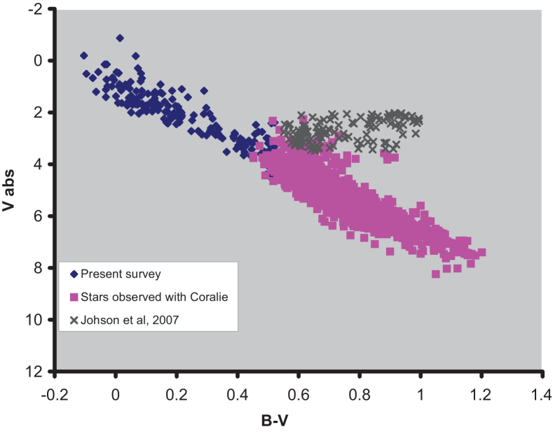
Figure 1: Observed stars in a HR diagram. We also plotted the dwarfs and/or (sub-) giants surveyed either with the Coralie spectrograph or by Johnson et al, 2006. Our targets cover a domain that was not surveyed yet. Note the relative lack of objects in the [0.2; 0.4] $B-V$ region, due to selection effects (see text)

2.3 Measurements

2.3.1 Radial velocities

The extraction of the radial velocities is fully described in Galland et al. 2005a . Briefly, for each star, we build a first estimate of the reference spectrum which is the average of the spectra recorded and reduced via the STS HARPS pipeline. We then compute a first estimate of the RV for each spectrum, by correlating in the Fourier space each spectrum and this first estimate of the reference spectrum. We then build a final reference spectrum by averaging the spectra once shifted from their measured RV. For each spectrum we finally measure the RV velocity with respect to this reference spectrum. We also measure the uncertainties associated to each RV measurement.

Note that to build up the reference we compute the $\chi^{2}$ of each spectrum compared to the first estimate of the reference spectrum. Most of the time, the $\chi^{2}$ found is much less than 10. Whenever a higher $\chi^{2}$ was found, we checked the spectra. In such cases, either they were due to bad observing conditions or technical problems and were not kept to build the reference spectrum (this actually happened quite rarely as we already selected spectra with acceptable absorptions) or they were associated to lines deformations indicative of a type-2 binary.

2.3.2 CCFs, bisectors and bisectors velocity-span

Whenever possible (see below) we computed for each target the resulting cross-correlation functions (CCFs) and the bisectors velocity-span (see for their definition Galland et al. 2005a ). Indeed, the bisector and bisectors velocity-span are very good diagnostics of stellar activity (spots, pulsations) provided 1) they can be measured (see below), and 2) the star projected rotational velocity is larger than the instrumental resolution (see Desort et al. (2007)).

The uncertainty associated to the bisectors velocity-span depends directly on the projected rotational-velocity and/or their spectra type. Indeed, the number of lines used to compute the CCF depends on these two parameters (much more than on the signal-to-noise ratio). For stars with high $v\sin{i}$ (typ. $\geq$ 150 km s^-1) and/or $B-V$ $\leq$ 0.1, the number of lines may be quite low (30–50) whereas for late-type stars with moderate $v\sin{i}$ (10–20 km s^-1), the number of lines used is a few hundreds (up to about 1 000). When the bisectors were computed, we then attributed quality flags to the bisectors velocity-span measurements, respectively: Good, Acceptable, Bad, corresponding to numbers of lines respectively $\geq$ 100, 40–100, and $\leq$ 40.

2.4 Diagnostics for the classification of variable stars

Variable stars are defined as having a RV standard deviation (rms) larger than twice the RV uncertainties and a total RV amplitude larger than 6 times the RV uncertainties. RV variations can a priori be due to the presence of a companion (star, brown dwarf, planet) or to intrinsic variations of the star (spots, pulsations). It can also be a combination of those different origins.

2.4.1 Binarity

We first checked those stars with high $\chi^{2}$ ($\geq$ 10) and looked for line deformations indicative of spectroscopic binaries. Figure 2 provides an example of a binary SB2 identified on the basis of the $\chi^{2}$, HD 2885 (A2V; $v\sin{i}$ = 40 km s^-1). It has to be noted that in such cases, the RV values measured are not any longer valid, as our RV extraction method assumes that all lines in a given spectrum originate from the same object.

For the rest of the variable stars, we tried to identify binary stars among the stars for which the RV amplitude can be explained by the presence of a stellar or BD companion. To do so, using rough estimations of the star masses via their $B-V$, we computed the RV amplitude 2$\times$$K_{\rm 2d}$ expected from the presence of a 13 M_Jup body orbiting with a period of 2 days and the RV amplitude 2$\times$ $K_{\rm 200d}$ expected in the case of a 200-days period and compared these quantities to the observed RV amplitudes, once corrected from the RV variations observed within a night (in practice, over a few hours), as the variations occuring within a few hours are assumed to be due to stellar origin, see below. Quantitatively we define as “in-night” RV amplitude for a given object, the amplitude of the nightly RV variations. We computed then the following quantities: $R_{\rm 2d}$ = (observed RV amplitude $-$ “in-night” RV amplitude)/ 2 $\times$$K_{\rm 2d}$ and $R_{\rm 200d}$ = (observed RV amplitude $-$ “in-night” RV amplitude)/ 2$\times K_{\rm 200d}$, to be used as thresholds to identify the binaries. Note that we chose 2 and 200-day periods as they are quite relevent given our temporal sampling and our average time baseline.

For those variable stars for which we could compute a CCF and test the relation between bisectors velocity-span and RV variations, we selected those that show a simple, flat bisectors velocity-span, i.e., values of bisectors velocity-span arranged horizontally in a (RV; bisectors velocity-span) diagram (this corresponds to stars for which the ratio of the amplitude of the bisector velocity span to the RV amplitude is smaller than 0.2) and for which $R_{\rm 2d}$ $\geq$ 2 or $R_{\rm 200d}$ $\geq$ 2; we regard them as unambiguous binaries. Figure 3 provides an example of a variable star (HD 68456; F5V; $v\sin{i}$ = 12 km s^-1) for which the bisectors velocity-span clearly indicates the presence of a companion and the observed RV amplitude once corrected from in-night variations can be due to a $\simeq$ 0.1 M_☉ stellar companion (see below). Note that this star was also recently classified as a binary on the basis of astrometric data (see below; Goldin & Makarov (2007)).

Some variable stars show a bisectors velocity-span which is either partly flat and partly vertical or partly flat and partly inclined, indicating that most probably they are binaries and at the same time pulsating or active (see below). We classify those objects with $R_{\rm 2d}$ or $R_{\rm 200d}$ $\geq$ 2 as strong binaries candidates. An example, HD 19545 (A3V; $v\sin{i}$ = 80 km s^-1), is provided in Fig. 4. Figure 5 shows for comparison the case of a pulsating star for which we artificially simulated an additional companion star. The generated RV and span curves of the pulsating star and pulsating star plus stellar companion are comparable to those found in the case of HD 19545. Note that we do not have quantitative criteria to identify those “composite bisectors velocity spans”; this is why we classify the candidates as strong candidates rather than unambiguous binaries.

Finally, for the rest of the stars, we flagged as binary candidates those stars with $R_{\rm 2d}$ or $R_{\rm 200d}$ $\geq$ 4. Note that for these stars we conservatively adopted a more stringent threshold for $R_{\rm 2d}$ or $R_{\rm 200d}$ as we lack of additional indication of the presence of companions, and we know that these stars may be intrinsically variable; we thus took into account the fact that the actual amplitude RV variations due to the pulsations may be larger than the one measured on our set of data. This ensures that most of the observed RV amplitudes is due to a perturbation by a BD or a star. Figure 6 gives an example of such a star.

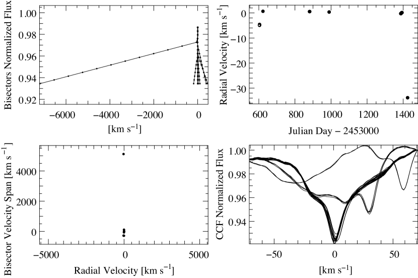
Figure 2: Example of an SB2 binary, HD 2885 (A2V; $v\sin{i}$ = 40 km s^-1). RV curve (upper right), CCFs (lower right), bisectors (upper left), and bisectors velocity-span (lower left). The CCF is clearly variable and indicative of an SB2 binary.

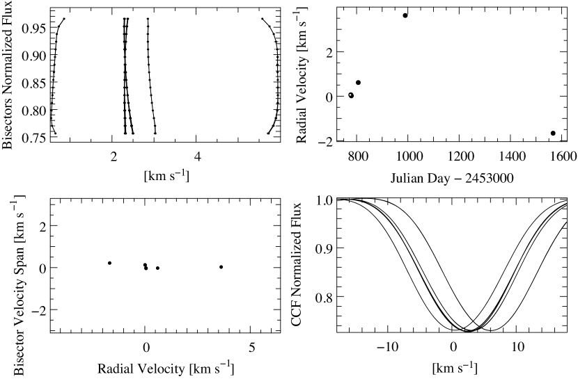
Figure 3: Example of a binary identified by a flat bisectors velocity-span diagram and high amplitude RV variations , HD 68456 (F5V; $v\sin{i}$ = 12 km s^-1). RV curve (upper right), CCFs (lower right), bisectors (upper left), and bisectors velocity-span (lower left). The mass of the companion falls in the stellar domain (see text).

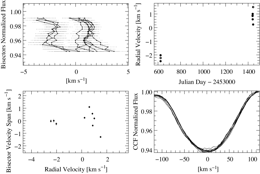
Figure 4: Example of a star whose RV variations are most probably due to both pulsations and binarity, HD 19545 (A3V; $v\sin{i}$ = 80 km s^-1). RV curve (upper right), CCFs (lower right), bisectors (upper left), and bisectors velocity-span (lower left). The CCFs are clearly variable; the bisectors velocity-span diagram is composite: part of the data are spread horizontally over a large velocity range, and part are spread vertically, over a large range of span . The points that give the vertical bisectors velocity-span are those associated to the nightly high frequency RV variations; their bisectors are strongly variable in shape. The points with the low RV are associated to bisectors spans that are clearly shifted from the ones corresponding to higher velocities; this produces a shifted bisectors velocity-span.

Figure 5: Simulation of a composite bisectors velocity-span diagram produced when adding a 100-M_Jup companion on a circular orbit, with a 120-day period around a 1.8-M_☉ pulsating star, HD 159492 (A7V; $v\sin{i}$ = 60 km s^-1). The initial RV and bisectors velocity-span data are showed on the left; we see in particular high frequency (nightly) RV variations and bisector velocity-spans spread vertically; the simulated data are showed on the right. The bisectors velocity-span diagram on the right is clearly composite: both flat over a wide range of RV + vertical over a wide range of span values, similarly to HD 19545.

Figure 6: Example of a star whose RV variations are most probably due to binarity, HD 200761 (A1V; $v\sin{i}$ = 80 km s^-1). RV curve. This is a case where no CCF could be computed, and the binarity classification relies solely upon the RV curve.

2.4.2 Planets

Those stars that shows at the same time signs of RV variability with low amplitudes and a flat bisectors velocity-span diagram are very good candidates for hosting planets. Note that in some cases, stars showing composite bisectors velocity-spans diagram with $R_{\rm 2d}$ or $R_{\rm 200d}$ larger than 2 can still be “good” candidates for hosting planets. In such cases, the total RV amplitude is not dominated by the planetary signatures but but stellar variability (e.g., spots).

2.4.3 Intrinsically variable stars

In the case of spots, and provided the star $v\sin{i}$ is higher than the instrumental resolution, the bisector shape is very peculiar and the bisectors velocity-span variations are correlated to the RV ones (see Desort et al. (2007)). In a (RV; bisectors velocity-span) diagram, the bisectors velocity-span values are arranged either as an inclined “8” shape, or along an inclined line (so called “anti-correlation”). For these objects, the ratio of the bisector span amplitude to the RV amplitude is found to be in the range 1–3. Figure 7 provides an example of a star showing clear signatures of spots on the basis of the bisectors velocity-span diagram (HD 25457; F5V; $v\sin{i}$ = 25 km s^-1). As another example, the very nice case of HD 138763 can also be found in Desort et al. (2007).

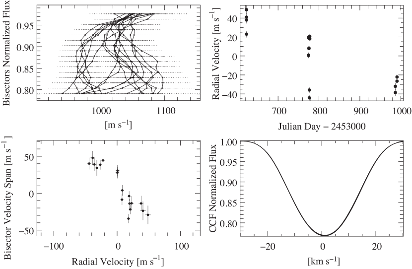
Figure 7: Example of a star with variable RV due to the presence of spots. HD 25457 (F5V; $v\sin{i}$ = 25 km s^-1). RV curve (upper right), CCFs (lower right), bisectors (upper left), and bisectors velocity-span (lower left). The bisectors velocity-span variations are clearly correlated to the RV variations.

In the case of pulsations, the bisectors velocity-span values are spread over a much larger range than the RV and their variations are not correlated to the RV ones. In a (RV; bisectors velocity-span) diagram, the bisectors velocity-span values are spread vertically, and the ratio of the bisector span amplitude to the RV amplitude is large, typically $\geq$ 3. Figure 8 provides an example of a pulsating star (HD 159492; A7V; $v\sin{i}$ = 60 km s^-1).

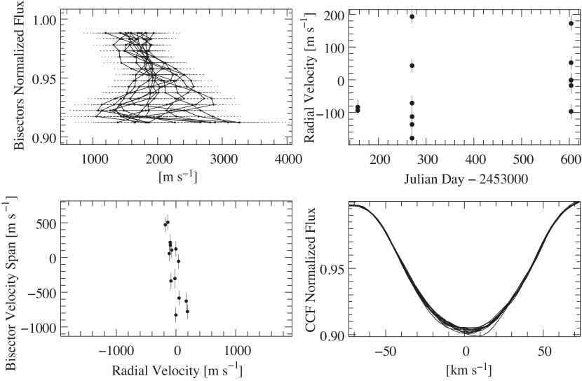
Figure 8: Example of a star with variable RV due to pulsations. HD 159492 (A7V; $v\sin{i}$ = 60 km s^-1). RV curve (upper right), CCFs (lower right), bisectors (upper left), and bisectors velocity-span (lower left). The CCF and bisector variations are due to line deformations; the bisectors velocity-span variations are not correlated to the RV variations.

3 Results

Given the variability criteria described above, 108 stars out of 170 are found to be variable in RV, and 62 are found to be constant in RV within our precision limits. Table LABEL:sample provides relevent measurements on these targets: RV amplitudes and uncertainties, bisector velocity-span rms and uncertainties.

3.1 Variability classification

3.1.1 Stellar binaries

20 stars are identified as binaries or candidate binaries with the criteria given in the previous section. More precisely:

• 4 binaries are found on the basis of the $\chi^{2}$ criterium, namely HD 99453, HD 209819, HD 2885 (Fig. 2), HD 142629.

• 6 stars show mostly flat bisectors velocity-span in a (RV; bisectors velocity-span) diagram: HD 11262, HD 68456, HD 41742, HD 116568, HD 216627, HD 54834. Their RV amplitude varies between 1 600 and 9 200 m s^-1.

• 4 stars have composite, flat+vertical bisectors velocity-spans in a (RV; bisectors velocity-span) diagram, together with a total RV amplitude dominated by the binarity effect. These pulsating binaries are: HD 220729, HD 12311, HD 19545 (Fig. 4) and HD 112934.

• Finally, 6 stars are classified as probable binaries on the sole basis of their RV variations: HD 158352, HD 177756, HD 158094, HD 2834, HD 200761 (Fig. 6), HD 116160.

The stars are flagged in Table LABEL:sample, and an indication on the criteria which was used to identify them as binaries or possible binaries is also given. No attempt was made to further characterize the stellar companion once the binary status was established, and no more data were recorded on the objects. Their RV variations are given in Figure 9.

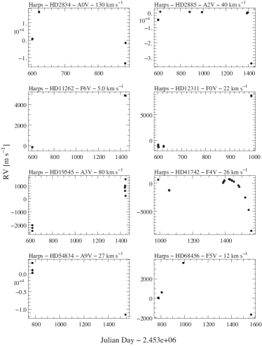
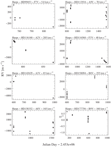
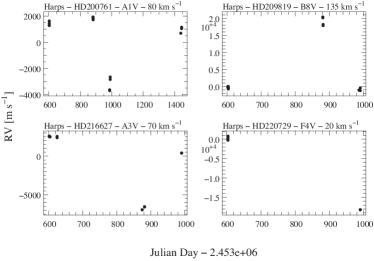
Figure 9: Radial velocity curves of the identified or strong candidates or probable binaries (see text).

Notes on some individual binaries (and potential binaries):

• HD 11262 is associated to a ROSAT source by Suchkov et al. (2003).

• HD 54834: Koen & Eyer (2002) (2002) reported this star as a photometric Hipparcos variable at a level of 0.0046 mag and with a frequency of 0.802 day^-1. Our data do not permit to confirm or infirm this frequency (not enough points, sampling not adapted).

• HD 68456 (Fig. 3) was not reported as binary in the Hipparcos catalog from the photometric and astrometric points of view; it is classified by Adelman (2001) as one of the Hipparcos least variable stars. Goldin & Makarov (2007) however provide an orbital solution to fit the Hipparcos astrometric data. The period found is 483$\pm$20 days, a₀ = 9.6${}^{+2.6}_{-1.2}$ mas, eccentricity = 0.12${}^{+0.25}_{-0.15}$, inclination = 131$\pm 16$$\degr$, $\omega$ = 103${}^{+72}_{-68}$$\degr$ and $\Omega$ = 171${}^{+164}_{-83}$$\degr$. Fixing the period and eccentricity proposed by these authors, we tried to find a fit to our RV data. They happen to provide good fits assuming a mass of $\simeq$ 100M_Jup for the companion.

• HD 99453: Baade & Kjeldsen (1997) questioned the previously suggested SB2 status of this object on the basis of their data; we do confirm the SB2 status for this star.

• HD 112934 (A9V; $v\sin{i}$ = 70 km s^-1): using Hipparcos photometry, Handler (1999) reports this star as a new possible $\gamma$ Doradus candidate but with a “weak complicated signal”, associated to a 0.8-day period. deCat et al. (2006) did not find clear line-profile variations in their CORALIE data. From our data, the star is both pulsating and member of a binary system, which makes the line-profile variations indeed more complicated than for pulsating stars. Our limited number of data does not permit to characterize the high-frequency period.

• HD 116160 was reported as an astrometric binary with accelerating proper motion by Makarov & Kaplan (2005).

• HD 116568 was classified as one of the least variable stars with Hipparcos by Adelman (2001). Baade & Kjeldsen (1997) report no variations in their $\pm$0.5 km s^-1 spectroscopic survey. The present data show that this star is a binary with an amplitude of at least 2 750 m s^-1. It is also reported as an unresolved Hipparcos problem star by Masson (1999) and associated to a ROSAT source by Suchkov et al. (2003).

• HD 142629 is an astrometric Hipparcos binary. It was also recently reported for the first time as a spectroscopic binary by Antonello et al. (2006).

• HD 158352 was classified as a possible Herbig AeBe star by The et al. (1994). Corporon & Lagrange (1999) in a survey of RV variations among Herbig AeBe stars did not find variations to a 5–10 km s^-1 level. This star was reported as being surrounded by a dusty disk by Oudmaijer et al. (1992), and Moor et al. (2006) give an age of 750$\pm$150 Myrs for the system.

• HD 177756 was classified as a possible $\lambda$ Bootis star, as well as a possible SB (Farragiana et al. (2004), Gerbaldi et al. (2003)). It is reported as one of the Hipparcos least variable stars (Adelman (2001)).

• HD 200761 was reported as one of the Hipparcos least variable stars (Adelman (2001)).

• HD 209819 was also reported as one of the Hipparcos least variable stars (Adelman (2001)).

• HD 220729 is associated to a ROSAT source by Suchkov et al. (2003).

3.1.2 Stars with planets

One star, HD60532 (F6IV–V; $B-V$ = 0.52) clearly reveals at the same time low-amplitude RV variations and flat bisectors velocity-spans diagram, indicative of the presence of two Jupiter mass companions with a high-confidence level. This star and the results of the fits of the RV curve is presented in Desort et al. 2008a . Interestingly in the frame of the present paper, the periods of the detected planets are long ($\geq$ 100 days). Hence, we get at least 1 $\%$ of F stars with long-period planets in our sample. This is much smaller than the predicted rate of $\simeq 10\,\%$ for 1.5 M_☉ stars by Kennedy & Kenyon (2008); however, we are yet not sensitive to all range of masses and periods as will be showed in the last section.

3.1.3 Single stars: intrinsic variability

We report in Table LABEL:sample the RV rms values obtained for each star, together with the associated uncertainties. Figure 10 provides for all the stars except those identified as binaries the measured RV rms as a function of their $B-V$, the ratio RV rms/uncertainties (E/I) as a function of their $B-V$ as well, and the ($B-V$; $v\sin{i}$) diagram for the same objects. In the plots we have distinguished the 88 stars that are found to be variable according to the criteria defined above and those 62 found to be constant according to the same criteria.

The E/I ratio varies between 1.5 and a few tens; it is relatively smaller for stars with small $B-V$ than for those with larger $B-V$. More quantitatively, the median value for this ratio computed on variable stars is 2.7 (resp. 4.4 and 5.2) for stars with $B-V$ $\leq$ 0.2 (resp. 0.2 $\leq$ $B-V$$\leq$ 0.4 and $B-V$$\geq$ 0.4). Hence we detect more variable stars among stars with large $B-V$ than stars with smaller $B-V$. We see moreover that the uncertainties generally increase with decreasing $B-V$. These results are not surprising and illustrate the fact that it is more difficult to identify variable stars when they have large uncertainties. In the frame of this study, it is important to keep in mind that our ability to detect variability generally decreases with decreasing $B-V$.

Note also that the uncertainties increase with increasing $v\sin{i}$; we could actually verify that the uncertainties vary as $v\sin{i}$ with a $(v\sin{i})^{\alpha}$ law where $\alpha=1.5\pm 0.1$, as predicted in Galland et al. 2005a .

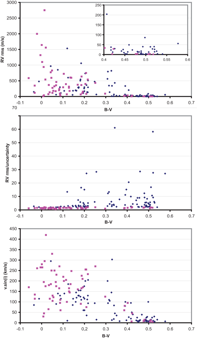
Figure 10: Top: RV rms measured for all stars but binaries with more than 6 spectra available as a function of $B-V$. Middle: Ratio RV rms/uncertainty for the same stars. Bottom: ($B-V$; $v\sin{i}$) diagram for the same stars. Losanges indicate RV variable stars and square indicate RV constant stars.

The percentage of variable stars depends on B$-$V in the following way:

• Most (85 $\%$) of the 58 stars with $B-V$ larger than 0.4 are found to be variable and the RV uncertainty is 2 m s^-1(median value). Evenmore, 90 $\%$ of the 46 stars with $B-V$ larger than 0.45, i.e., well beyond the instability strip, are found to be variable and their uncertainty is 1.4 m s^-1(median value). We conclude then that at a level of precision of 2 m s^-1or less, most of the stars with $B-V$ larger than 0.4 are RV variable.

• Among the stars with $B-V$ between 0.2 and 0.4, the number of variable stars found is small, but this is due to a selection effect as known $\delta$ Scuti and $\gamma$ Doradus stars were removed from our sample (see above).

• Only 36 $\%$ of the 73 stars with $B-V$ smaller than 0.2 are found to be variable. The percentage of variable decreases to 20 $\%$ if we consider the 40 stars with $B-V$ smaller than 0.1. For those stars with $B-V$ between 0.1 and 0.2, we get as many variable as constant stars. The number of stars found to be constant according to our criteria increases then with decreasing $B-V$. However, we have seen that our ability to detect variable stars decreases with decreasing $B-V$. More quantitatively, the median uncertainty in the case of “constant” stars is $\simeq$ 290 m s^-1 whereas the median uncertainty in the case of stars found to be variable is $\simeq$ 80 m s^-1. Furthermore, the median uncertainty of constant stars is comparable to the median value of the standard deviation of variable stars (265 m s^-1). Hence we may stipulate that in fact most of the stars with $B-V$ $\leq$ 0.2 are probably RV variable.

When the CCF and bisectors velocity-span criteria apply (in fact, whenever the bisectors velocity-span can be measured with a good or acceptable quality), we may try to further characterize the stellar variability. We find that in such cases, as expected, most of the variable stars with $B-V$ smaller than 0.3 show signs of pulsations, whereas most of the variable stars with higher $B-V$ show signs of spots.

3.2 Variability of stellar origin and impact on planet detectability

Table 2: Median values of RV rms (second row) and RV uncertainties (third row) for stars with more than 6 spectra (3 epochs) available. The number of stars per bin of $B-V$ is also given (first row). Rows 7–9 give the median per bin of $B-V$ of the achievable detection limits deduced from the measured rms for each star, expressed in Jupiter mass. Three periods are considered: 3, 10 and 100 days (see Sect. 3). Note that we assume that the planet, supposedly on a circular orbit, is detectable if the amplitude of the RV variations is larger than $3\times RVrms$. Rows 7–9 give the percentage of stars for which the detection limit, given the measured RV rms, fall in the planetary domain.

$B-V$	[$-$0.1; 0]	[0; 0.1]	[0.1; 0.2]	[0.2; 0.3]	[0.3; 0.4]	[0.4; 0.5]	[0.5; 0.6]
number of stars	7	31	32	16	17	30	17
median RV rms (m s-1)	480	298	283	330	66	13	4
median RV uncertainty (m s-1)	239	300	90	80	19	2	1.4
median detection limit ($P$ = 3 days)	10	5	4.5	5	0.8	0.17	0.05
median detection limit ($P$ = 10 days)	15	8	7	7	1.3	0.25	0.08
median detection limit ($P$ = 100 days)	31	17	15	16	2.8	0.55	0.17
percentage (3 days)	71	71	94	100	100	100	100
percentage (10 days)	43	68	78	88	88	100	100
percentage (100 days)	28	42	44	37	60	100	100

The “uncorrected” jitters, as given directly by the measured RV rms are provided in Table LABEL:sample, for each star, together with the associated uncertainties. Note that we prefer not to use the jitters corrected from the uncertainties, as sometimes done, as our main aim is to evaluate the impact on planet detectabiliity rather than to make stellar studies. Table 2 gives the computed median “uncorrected” jitters per bins of $B-V$.

In Galland et al. 2005a we had shown that the detection limit strongly depends on the star ST and its projected rotational-velocity; more precisely, the detection limit increases with earlier ST and/or larger $v\sin{i}$. Thanks to the present data, we can in addition address the question of the impact of the stellar jitter.

To estimate the detectable masses for a given star and a given period, we assume that a planet, supposedly on a circular orbit is detectable if the amplitude (2$\times K$) of RV variations that it would produce is larger than 3$\times$ RV rms, where RV rms is the ”uncorrected” jitter actually measured. We will come back later on the validation on this assumption. We give for each star in Table 3 the computed detectable limits assuming 3-day, as well as 10-day and 100-day periods. Figure 11 shows the detection limits for all stars for a 3-day period. For comparison, we also give in this figure the mass of the planet that would be detectable if the star is not active/pulsating (hence has no jitter) and the limit would then be set by the uncertainty (hypothesis 2$K$ = 3$\times$ uncertainty). The ratio of the two values is E/I. As previously seen, this ratio is larger than 1.5 and may be quite high; the impact of the jitter on the detectable masses is therefore non negligeable.

Several comments can be made:

• the achievable limits fall into the planetary domain for a large number of stars: more precisely, in 137 out of 150 stars, i.e., 91 $\%$, the detection limit for a 3-day period falls within the planetary domain. For the remaining stars the limit falls well into the BD domain with masses up to 54 M_Jup. When considering a 10-day (resp. 100-day) period, we find that we can reach the planetary mass domain for 124 stars, hence 83 $\%$ (resp. 92 stars, hence 61 $\%$). For a 10-day period, the limit for all remaining stars but one fall into the BD regime; for the 100-day period, the limit for all remaining stars but 6 fall in the BD domain.

• as expected, the median of the detection limits generally improve with increasing $B-V$, from 10 M_Jup for $B-V$ between -0.1 and 0, to 5 M_Jup for $B-V$ between 0 and 0.3, to 0.05 M_Jup for $B-V$ between 0.5 and 0.6 (for a 3 day period) (see Table 2). Noticeably, for stars with $B-V$ $\geq$ 0.3, individual detection limits may be as low as 0.02 M_Jupand for stars with $B-V$ $\leq$, 0.3, individual detection limits may be as low as 0.5 M_Jup. For a ten day period, these numbers become respectively: 15, 7 and 0.08 M_Jup; for a 100 day period, 31, 16 and 0.17 M_Jup. Also, noticeably, the detection limits steeply improves at $B-V$ = 0.3.

• the ”uncorrected” jitter varies a lot from one object to the other. Therefore the general conclusion that the detection limits improves with increasing $B-V$ may not apply when considering individual objects: for instance, the two stars HD 50445 (A3V; $B-V$ = 0.18) and HD 63847 (A9V; $B-V$ = 0.3) have similar projected rotational-velocities ($v\sin{i}$ $\simeq$ 90 km s^-1) and very different levels of activity, with an RV rms of 66 m s^-1 and 794 m s^-1 respectively. When we take this ”uncorrected” jitter into account, the detection limit is 1 M_Jup ($P=3$ days) and 1.5 M_Jup ($P=10$ days) around the A3V star whereas the detection limit is about 10 times higher for the A9V star.

We conclude then that planets can indeed be found around a wide range of stars with $B-V$ larger than $-$0.1, even taking into account their jitter. The achievable detection limit of such early type stars cannot be predicted given only the star properties (ST, $v\sin{i}$), but requires to record data to estimate their level of jitter.

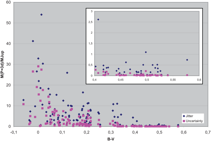
Figure 11: Achievable detection limits for all stars but binaries taking into account their actual ”uncorrected” jitter (losanges) or the measured uncertainties (squares), and assuming a planet on a circular 3-day orbit.

Note: we note that of course, the measured ”uncorrected” jitter provides a reliable limit to planet detection only when this jitter is due to stellar activity in general, and not to companions. Would a companion be present, its contribution to the RV variability would have to be removed in order to estimate the impact of the stellar activity.

4 Planet detection limits of the present survey

4.1 Estimation of the achieved detection limits

We try now to estimate the detection limits reached by the present survey, taking into account the actual RV curve. For each star, we then compute the detection limit (companion mass) as a function of its period. To do so, we consider a planet with a given mass and with a given period (the orbit is assumed to be circular). For any couple (Mass; Period) we generate a large number of keplerian orbits, assuming different times of passage at periastron ($T_{0}$). For each orbit, we compute the expected radial velocities at the times of the actual observations. We add a noise (random value between ${}^{+}_{-}$ RV uncertainty), where RV uncertainty is the uncertainty measured on the RV data. We then get a virtual set of RVs, which takes into account the star properties (in particular, its ST and rotational velocity, through the uncertainties and SN). We compute then the standard deviation of the virtual RVs points. For a given (Mass; Period), the distribution of all the standard deviations (corresponding to differents $T_{0}$) obtained is gaussian. We compute then the average value of the distribution of the virtual standard deviations. We consider that a planet with a given (Mass; Period) is detectable if the standard deviation of the real RV values is smaller than the average value of the virtual standard deviations. We determine the confidence level (or detection probability) associated to such an orbit by comparing the standard deviation of the virtual distribution with the difference between the standard deviation of the real RV measurements and the average value of the virtual standard deviations.

In practice, for a given object, we explore 200 periods in the range 0.5 to 1000 days, and 100 planet masses in the range (Mmin; 100 M_Jup) where Mmin corresponds to the achievable mass given the measured uncertainty. For a given (Mass; Period), we explore 1000 $T_{0}$. We checked that increasing the number of periods, or planet masses and or initial $T_{0}$ does not significantly impact the results.

For each (Mass; Period) couple, we obtain thus a detection probability. In a (Mass; Period) diagram, we can then identify the domain where a planet with a given mass and period should be detectable if present, with a given level of confidence. This defines then a domain in which we can exclude the presence of a planet with a given level of confidence. We will consider two levels of confidence: 1$\sigma$, (i.e., a 68.2 $\%$ probability) and 3$\sigma$ (i.e., 99.7 $\%$ probability).

4.2 Sensitivity of the survey and first constrains on early type stars

The sensitivity of our survey is a consequence of the number of data available and on the temporal sampling of the data. We kept only those stars (107 objects), found to be either constant or variable, for which we got more than 12 data points (6 epochs). Also, given the data at hand, we limited the range of periods investigated between 1 days and a few hundred days. We report in Table 3 the achieved limits (68.2 $\%$ and 99.7 $\%$ probabilities) obtained for each of the 107 stars considering three periods: 3, 10 and 100 days.

We give also in Fig. 12 examples of achieved detection limits (68;2 $\%$ and 99.7 $\%$ probabilities) as estimated with the previously described simulations. We have also plotted on the figures the achievable detection limits taking into acount the jitter, as defined in the previous section, as well as the detection limits corresponding to the measured uncertainties. We recall that the last two cases (achievable limits) do not take into account the actual temporal sampling of the data, conversely to the detection limits computed with our virtual realisations.

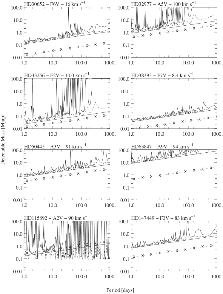
Figure 12: Detection limits. X-axis: periods (days). Y-axis: Detection limit (M/M_Jup). Curve: detection limits actually achieved in the present survey; plain curves correspond to 99.7 $\%$ detection probability, and broken curves to 68.2 $\%$ probability. Note that the RV data were beforehand averaged over one day. Straight line: achievable detection limits assuming a 3$\times$ rms threshold for the planet amplitude. Line with crosses: achievable detection limits assuming a 3$\times$ uncertainty threshold for the planet amplitude.

When enough data are available, the actual detection limits fall close to the achievable limits obtained assuming the $3\times{\rm RV}$ rms threshold for the amplitude of RV variations, as can be seen in Fig. 12. This justifies the choice of the threshold adopted in the previous section to estimate the achievable limits.

Note that we sometimes endup with high detection limits that fall outside the investigated range of masses, i.e., $\geq$ 100 M_Jup when we consider a period of 100 days whereas the detection limits for a 3 or 10 days period are close to the achievable limits. This corresponds to cases where the temporal sampling is not adapted to explore such a long period (see for instance the case of HD 33256, in Fig. 12). It sometimes, but much less frequently also happens that the detection limit for a 10 days fall outside the investigated range of masses whereas the detection limits for a 3 days period is close to the achievable limit. In fact, our survey allows to search mostly for short-period planets (typ. a few days); 10–100 day periods are not always sampled enough to get interesting results (especially on early-type stars) and $\geq$ 100-day periods are not properly sampled to get interesting results. We will therefore in the following discuss only periods $\leq$ 100 days. Finally, one has to note that in some cases, we get a 99.7 $\%$ probability detection limit out of the investigated range, where as the 68.2 $\%$ limit fall well into the investigated range. This happens generally when the number of data is the lowest: 12 or 14.

To study the impact of $B-V$ on the present results, we computed the percentage of stars for which the achieved detection limits (68.2 $\%$ and 99.7 $\%$ probabilities) fall in the planetary or BD domains per bin of $B-V$, considering a 3-day, a 10-day and a 100-day periods. We also computed the median of the achieved detection limits (considering 68.2 $\%$ and 99.7 $\%$ probabilities) per bin of $B-V$ for such periods. The results are given in Table 4. In order to allow comparison between the limits obtained with these two probabilities and with the achievable ones, we considered for the computation of the median values only those stars for which both the 68.2 $\%$ and 99.7 $\%$ probabilities detection limits fall into the investigated range of masses. Finally, one has to note that for the earliest type stars, the number of objects per bin is quite small, so one has to be very cautious with the associated statistics. We can see that:

• if we consider a 3-day period, the achieved limit at 1 (resp. 3) $\sigma$ fall in the planetary domain for 90 $\%$ (resp. 81  $\%$) of the stars. This percentage is quite comparable to the one found in Sect. 3. It increases from 75 (resp. 25) $\%$ for the earliest type stars to 100 (resp. 100)  $\%$ for stars with $B-V$ larger than 0.3. Also, the median of the achieved limits at 1 (resp. 3) $\sigma$ decreases from 7 (resp. 7) M_Jup for the earliest-type stars to 0.08 (resp. 0.3) M_Jup for the latest-type stars. Moreover, the steep step seen in Sect. 3 in the detectable masses at $B-V$ = 0.3 is also clear.

• if we consider a 10-day period, the achieved limit at 1 $\sigma$ (resp. 3) fall in the planetary domain for 82 $\%$ (resp. 67 $\%$) of the stars. This percentage increases from 50 (resp. 25) $\%$ for the earliest type stars to 100 (resp. 100)  $\%$ for stars with $B-V$ larger than 0.4, with however an exception on the [0.2; 0.3] range where it decreases back to 50 $\%$. Also, the median of the achieved limits at 1 (resp. 3) $\sigma$ decreases from 12 (resp. 24) M_Jup for the earliest-type stars to 0.1 (resp. 0.7) for the latest-type stars, with however an exception in the range [0.2; 0.3] range as regards the 99.7 $\%$ probability. Again the steep step is observed at $B-V$ = 0.3.

• if we finally consider a 100-day period, the achieved limit at 1 (resp. 3) $\sigma$ fall in the planetary domain for 54 (resp. 35) $\%$ of the stars. We note that this percentage is smaller than the one obtained in Sect. 3 and attribute the discrepancy to the actual temporal sampling and the relatively small amount of targets investigated yet. The median of the achieved limits at 1 (resp. 3) $\sigma$ decreases from 19 (resp. 34) M_Jup for stars with $B-V$ $\geq$ 0.0 to 1. (resp. 1.9) M_Jup for the latest-type stars. Again the steep step is observed at $B-V$ = 0.3.

Table 4: Percentage of stars for which the achieved detection P=68.2$\%$ or P=99.7$\%$ limits fall in the planetary or BD/planet domains. Three periods are considered: 3, 10 and 100 days. Median values of the achieved detection limits, expressed in Jupiter mass, per bin of $B-V$. For the these median values, we took into acount only the stars for which both the P=68.2$\%$ and P=99.7$\%$ limits fall into the investigated companion mass range. The corresponding number of stars is given as well as the median achievable limits for those stars.

$B-V$	[$-$0.1; 0]	[0; 0.1]	[0.1; 0.2]	[0.2; 0.3]	[0.3; 0.4]	[0.4; 0.5]	[0.5; 0.6]
Number of stars (whole sample)	4	19	21	10	12	24	17
$P=3$ days
Percentage of limits in the planet domain	75;25	74;47	95;61	100;60	100;100	100;100	100;100
(P=68.2$\%$;P=99.7$\%$)
Percentage of limits in the BD/planet domain	100;100	100;100	100;100	100;100	100;100	100;100	100;100
(P=68.2$\%$;P=99.7$\%$)
$P=10$ days
Percentage of limits in the planet domain	50;25	58;42	80;52	50;30	92;66	100;100	100;100
(P=68.2$\%$;P=99.7$\%$)
Percentage of limits in the BD/planet domain	100;100	100;52	100;95	100;64	100;92	100;92	100;100
(P=68.2$\%$;P=99.7$\%$)
$P=100$ days
Percentage of limits in the planet domain	25;0	16;10	28;10	30;10	58;33	92;55	94;47
(P=68.2$\%$;P=99.7$\%$)
Percentage of limits in the BD/planet domain	75;25	74;83	95;48	100;40	100;58	100;59	100;100
(P=68.2$\%$;P=99.7$\%$)
$P=3$ days
Number of stars	4	17	17	8	11	22	17
Achieved detection limit (P=68.2$\%$)	6.9	5.3	5.1	3.2	0.5	0.25	0.08
Achieved detection limit (P=99.7$\%$)	6.9	12.1	7.3	6.3	1.0	0.3	0.3
Achievable detection limit	6.9	5.5	4.2	2.5	0.4	0.2	0.06
$P=10$ days
Number of stars	4	14	20	7	11	22	17
Achieved detection limit (P=68.2$\%$)	11.7	8.0	7.2	4.4	0.9	0.4	0.1
Achieved detection limit (P=99.7$\%$)	24.0	11.8	10.2	17.4	2.0	0.8	0.7
Achievable detection limit	10.3	6.9	5.6	4.1	0.6	0.3	0.1
$P=100$ days
Number of stars	1	6	11	5	8	13	12
Achieved detection limit (P=68.2$\%$)	(10.0)	18.7	17.3	14.2	5.2	1.1	1.0
Achieved detection limit (P=99.7$\%$)	(17.6)	34.4	32.9	33.8	20.4	2.4	1.9
Achievable detection limit	(8.5)	15.0	10.5	8.9	3.0	0.8	0.6

Finally, we give the probability not to detect planets of a given mass and with a given period (3, 10, 200, 500 days) around stars with a given spectral type and $v\sin{i}$. The results are summarized in Table 5. We see that as expected, for a given probability, the limits globally decrease with increasing B$-$V and decreasing $v\sin{i}$.

Table 5: Detection limit for 50 $\%$ and 90 $\%$ for different periods. The last column give the number of stars considered to estimate these detection limits. Note that only stars with more than 12 measurements (6 epochs) were considered. Binaries were excluded. Also note that numbers outside the planetary mass domain ($>13$ M_Jup) are not given.

ST, $v\sin{i}$	Period	50 $\%$	90 $\%$	N-st.
	[days]	[MJup]	[MJup]
early A, $v\sin{i}$ $\leq$ 70 km s-1	3	1.2	–	2
	10	1.7	–	2
	200	4.7	–	2
	500	6.4	–	2
early A, $v\sin{i}$ 70-130 km s-1	3	4.6	7.2	9
	10	6.9	10.7	9
A, $v\sin{i}$ $\leq$ 70 km s-1	3	3.5	–	2
A, $v\sin{i}$ 70-130 km s-1	3	4.5	6.3	10
	10	6.7	9.5	10
A, $v\sin{i}$ $\geq$ 130 km s-1	3	11.2		13
F, $v\sin{i}$ $\leq$ 15 km s-1	3	0.1	0.8	28
	10	0.2	1.2	28
	200	0.4	3.2	25
	500	0.6	2.7	22
F, $v\sin{i}$ 15-60 km s-1	3	0.6	0.8	13
	10	0.9	1.2	13
	200	2.8	3.3	12
	500	3.8	4.5	12
F, $v\sin{i}$ $\geq$ 60 km s-1	3	1.9	10.2	10
	10	2.8		10
	200	7.5		9
	500	10.1		9

Obviously, the statistics provided by our survey is still poor on early type stars, and still very limited on the latest type stars. Concerning the latter, we note that if we consider the 41 objects with $B-V$ $\geq$ 0.4, i.e., well beyond the instability strip, we find that less than 24 $\%$ of stars host planets with masses equal to 0.5 M_Jup or more; less than 5 $\%$ host planets with masses equal to 1 M_Jup or more on a 3-day period. For a 10-day period, we find that less than 42 $\%$ host planets with masses $\geq$ 0.5 M_Jup, and less than 20 $\%$) host planets with masses $\geq$ 1 M_Jup. The comparison between achieved and achievable detection limits shows that there is still room to significantly improve those statistics (thanks to new data points).

The present statistics certainly does not allow quantitative comparisons with late type dwarfs, which have been surveyed by several groups since more than 10 years, or with giant or sub giant stars, because in that case of the lack of data for both massive dwarfs and (sub-)giants.

Concerning the presence or absence of hot Jupiters around massive stars, we note that the planets found so far in our survey are located at about 0.7 AU or more from a 1.4 M_☉ star; this separation corresponds to that of the closest planet found around giant stars. We also detected recently a planet orbiting at 0.6 AU from a dwarf with a similar mass in the northern hemisphere (Desort et al. 2008b ). Due to the still limited amount of data available, it should not be concluded however that there are no planets closer to massive dwarfs. We also recall that a few short period planets have been found around 1.4 M_☉ stars through transits.

5 Conclusion

Based on the observation of a large number of A–F type stars (170), we have been able to measure their jitters, and derive for the first time estimations of the detection limits that can be expected on average on those stars with $B-V$ in that range [$-$0.1; 0.6] (once previously known $\delta$ Scuti and $\gamma$ Doradus stars are removed) for 3 periods: 3, 10 and 100-day periods. We have shown that at the precision provided by HARPS, most of the stars are variable in RV, and the impact of the RV jitter, due to either spots or pulsations is generally non negligeable on planet detectability. However, assuming that planets are detectable if the amplitude of the induced RV variation is larger than 3$\times{\rm rms}$ (this threshold defines the achievable detection limits, which depends on the star and the spectrograph used), we have shown that even when taking into account the jitter, giant planets can still be found around these stars in most cases. This is not only true for the stars with $B-V$ $\geq$ 0.3 for which we can find either short or long period planets, with masses as small as 0.02 M_Jup (case of short period) for the latest type stars but also for dwarfs with $B-V$ $\leq$ 0.3: for such stars short-period planets can still be found around those with relatively low projected rotational-velocity and low level of activity, with masses down to 0.5 M_Jup (best case). This survey has allowed to identify for the first time the stars that are best suited for further searches for planets around massive dwarfs.

We have also shown that given the data available, the present survey is sensitive to short-period planets (hot Jupiters) and only partially sensitive to larger periods (up to 100 days). We found in particular one 2-planet system with periods larger than 100 days around one late-type star. Whenever possible (107 stars), we computed for each star the detection limits actually achieved and showed that when enough data are available, the achieved detection limit is set by the $3\times{\rm rms}$ threshold. We indeed reached such limits for early-type as well as for late-type stars. We finally derive first estimates of the presence of short-period planets around these A–F stars. We showed for instance that less than 5 $\%$ of the latest-type stars ($B-V$ $\geq$ 0.4) host P=3 days-period planets with masses 1 M_Jup or more. Such statistics are not constraining enough to allow interesting comparisons with later type stars or with model predictions; but as soon as more data become available, the statistics can be straightforwardy improved.

Finally, we note that to compute these detection limits, we did not try to average out the spectra over timescales associated to the frequencies of intrinsic stellar variations. This approach would of course allow to decrease significantly the detectable masses. As it would require lots of telescope time, it should be probably kept for stars with the highest scientific interest.

Table 6: Stars properties and measurements. “RV rms” (resp. “span rms”) stands for the rms of the measured radial velocities (resp. bisector velocity-spans); “RV amp” (resp. “Span amp.”) stands for amplitude of the measured radial velocities (resp. bisector velocity-spans); “RV unc.” (resp. “Span unc.”) stands for the average uncertainties associated to the RV (resp. bisector velocity-spans) data. Bisector flags: G: good quality; B: bad quality; A: acceptable quality. Binary types: X refers to stars identified as binaries based on a high $\chi^{2}$ ($\geq$ 10); B refers to binaries identified via a flat or a composite bisector, and V refers to stars regarded as binary candidates, based on the sole amplitude of their RV variations (see text).

HD	ST	$B-V$	$v\sin{i}$	Time	RV	RV	RV	Span	Span	Span	Bis.	Variabl.	Bin.
				bs l	rms	unc	ampl	rms	unc	ampl	Flag
			(km s-1)	(days)	(m s-1)	(m s-1)	(m s-1)	(m s-1)	(m s-1)	(m s-1)
HD 693	F5V	0.487	10	389.1	2	1	6	2	1	7	G	V
HD 2696	A3V	0.128	150	389.1	279	166	847					C
HD 2834	A0V	0.018	130	279.2	9408	164	29717					V	V
HD 2884	B9V	-0.06	170	603.2	587	496	2141					C
HD 2885	A2V	0.147	40	820.7	9331	19	34510				B	V	X
HD 3003	A0V	0.038	115	603.2	135	83	491					C
HD 4247	F0V	0.35	35	842.8	26	11	94	62	49	216	G	V
HD 4293	A7V	0.297	125	837.8	91	99	270	4109	1281	16151	B	C
HD 7439	F5V	0.448	8	453.8	10	1	22	24	2	63	G	V
HD 9672	A1V	0.066	195	453.8	169	300	527					C
HD 11262	F6V	0.523	5	840.8	2500	1	5014	30	2	64	G	V	B
HD 12311	F0V	0.29	22	387.9	3674	80	10137	3113	757	12217	G	V	B
HD 13555	F5V	0.457	9	821.8	13	1	42	20	3	54	G	V
HD 14943	A5V	0.213	111.5	835.8	141	50	667	745	484	6364	A?	V
HD 15008	A3V	0.034	180	1165.9	367	274	1210					C
HD 17848	A2V	0.101	220	842.8	294	194	1046					C
HD 18978	A4V	0.163	120	1161.8	185	88	880	13988	1317	105268	B	V
HD 19107	A8V	0.193	170	389	154	176	434					C
HD 19545	A3V	0.166	80	821.9	1490	33	3962	623	244	2389	A	V	B
HD 21882	A5V	0.205	255	382.9	400	350	1332					C
HD 25457	F5V	0.516	25	368.1	28	3	93	28	8	82	G	V
HD 25490	A1V	0.032	65	5	74	71	214					C
HD 29488	A5V	0.147	115	665.2	183	72	712	3160	855	23124	B	V
HD 29875	F2V	0.342	45	325	434	7	1100	1108	36	2551	G	V
HD 29992	F3V	0.391	100	638.2	335	30	855	319	226	1386	G	V
HD 30652	F6V	0.484	16	500.7	13	2	54	19	7	90	G	V
HD 30739	A1V	0.01	195	328	941	631	3380					C
HD 31746	F3V	0.442	11.4	295	18	2	60	45	6	144	G	V
HD 32743	F2V	0.421	50	663.2	13	5	44	145	42	441	A	V
HD 32977	A5V	0.118	100	175.7	70	47	279	272	340	990	A/B	C
HD 33256	F2V	0.455	10	326	4	2	14	5	4	16	G	V
HD 33262	F7V	0.526	30	665.1	17	3	45	60	7	173	G	V
HD 37306	A2V	0.051	130	670.2	275	180	1127					C
HD 38393	F7V	0.481	8.4	1165.9	4	1	19	5	2	22	G	V
HD 38678	A2V	0.104	200	338.1	723	429	1942					C
HD 39014	A7V	0.217	205	665.2	512	173	2376					V
HD 39060	A3V	0.171	130	670.1	287	39	996	883	423	3702	A	V
HD 40136	F1V	0.337	18	663.2	10	3	36	19	7	77	G	V
HD 41695	A0V	0.046	250	280.2	595	628	2046					C
HD 41742	F4V	0.493	26.3	450.9	673	5	2030	44	17	148	G	V	B
HD 43940	A2V	0.139	247.5	282.2	597	513	1939					C
HD 46089	A3V	0.185	110	0.1	1060	64	2618	3148	687	8811	A	V
HD 49095	F7V	0.491	7	337.9	3	1	13	4	2	21	G	V
HD 49933	F2V	0.396	12	29	29	2	85	83	4	237	G	V
HD 50445	A3V	0.183	90.7	670.1	66	36	248	301	295	1672	A	C
HD 54834	A9V	0.312	26.9	0.9	1183	11	2839	127	657	312	G	V	B
HD 56537	A3V	0.106	140	666.2	180	75	639	3198	1090	15172	A	V
HD 59984	F5V	0.54	15	29.9	3	1	10	30	24	107	B	V
HD 60532	F6V	0.521	10	667	26	1	109	4	2	22	G	V
HD 60584	F6V	0.468	38.9	663.1	23	9	83	62	44	215	G	V
HD 63847	A9V	0.31	94	339	794	65	3145	997	565	3835	A	V
HD 66664	A1V	0.018	175	32.8	542	450	1695	0	0	0		C
HD 68146	F7V	0.488	8	666.1	4	1	16	5	3	27	G	V
HD 68456	F5V	0.437	12	212.3	1236	2	3613	70	4	177	G	V	B
HD 71155	A0V	-0.012	115	337.9	480	227	2288					V
HD 73262	A1V	0.003	265	30.9	1101	777	3843					C
HD 74591	A6V	0.2	115	338	171	80	639	726	901	3137	B	V
HD 74873	A1V	0.12	10	28.9	1534	114	5167	0	0	0		V
HD 75171	A9V	0.217	93.3	388	294	57	934	713	443	2021	A	V
HD 76653	F6V	0.481	11	282.1	13	1	45	14	3	55	G	V
HD 77370	F3V	0.417	95	667.1	37	15	134	136	71	504	G	V
HD 82165	A6V	0.216	232.8	32	541	276	2046					C
HD 83446	A5V	0.173	155	670.1	274	83	1152					V
HD 88955	A2V	0.051	105	99.8	115	69	450					C
HD 89328	A8V	0.329	302.8	568.3	340	93	956					V
HD 90132	A8V	0.251	270	28.9	433	221	1647					C
HD 91324	F6V	0.5	8	665.1	3	1	13	6	3	25	G	V
HD 91889	F7V	0.528	6	665	4	1	17	2	1	9	G	V
HD 93372	F6V	0.51	11.3	638.1	4	2	14	8	5	28	G	C
HD 94388	F6V	0.48	8	31.9	15	1	51	27	3	79	G	V
HD 96819	A1V	0.069	230	5	463	442	1520					C
HD 97244	A5V	0.209	75	106.8	84	45	298	301	360	1246	A	C
HD 97603	A4V	0.128	165	32.9	315	170	987	0	0	0		C
HD 99211	A9V	0.216	130	29.9	135	59	474	433	592	1796	A	V
HD 99453	F7V	0.495	5	32	253	1	784					V	X
HD 100563	F5V	0.48	14	564.3	3	2	10	12	4	35	G	C
HD 101198	F7V	0.52	5	662.1	40	1	102	2	1	5	G	V
HD 102124	A4V	0.174	130	29.9	297	114	1195	2230	1928	7132	B	V
HD 102647	A3V	0.09	115	106.8	111	44	426	419	454	2305	A	V
HD 104731	F6V	0.417	20	29.9	23	2	75	129	6	445	G	V
HD 105850	A1V	0.055	122	569.3	181	107	606					C
HD 106661	A3V	0.068	175	32	358	373	1272					C
HD 109085	F2V	0.388	81	638	22	15	77	86	82	329	G	C
HD 109787	A2V	0.049	330	32.9	829	509	3038					C
HD 110411	A0V	0.076	140	32.9	851	415	2748					V
HD 111998	F5V	0.493	28.5	638.1	40	5	144	35	18	128	G	V
HD 112934	A9V	0.298	70	73.8	857	43	2877	580	289	1950	G	V	B
HD 114642	F6V	0.46	13	105.7	49	2	194	118	4	448	G	V
HD 115892	A2V	0.068	90	101.8	59	29	232					V
HD 116160	A2V	0.045	205	97.7	4080	437	10844					V	V
HD 116568	F3V	0.415	40	74.9	1243	8	2751	154	36	592	G	V	B
HD 118098	A3V	0.114	205	105.9	395	263	1533					C
HD 124850	F7V	0.511	15	5	39	2	129	88	6	278	G	V
HD 125276	F7V	0.518	5	182.8	1	1	4	2	1	8	G	C
HD 126248	A5V	0.124	185	280.2	602	204	2482					V
HD 128020	F7V	0.506	5	73.8	2	1	6	3	2	10	G	C
HD 128167	F3V	0.364	8	6	21	3	70	56	5	169	G	V
HD 128898	F1V	0.256	15	0.1	64	2	189	41	6	121	G	V
HD 129422	A7V	0.308	200	113.9	562	196	1742					V
HD 129926	F0V	0.315	110	73.9	347	26	1074	642	214	2358	G	V
HD 130109	A0V	-0.005	265	31	1319	945	4253					C
HD 132052	F0V	0.318	105	182.6	139	31	496	495	253	1490	G	V
HD 133469	F6V	0.489	24.3	182.6	17	5	60	32	17	104	G	V
HD 135379	A3V	0.088	60	841.8	31	22	105	109	153	435	G	C
HD 135559	A4V	0.181	125	389	505	87	2063	1626	1166	6894	B	V
HD 138763	F7V	0.577	7	623.2	56	2	200	54	4	217	G	V
HD 139211	F6V	0.505	7	182.7	3	1	12	3	2	12	G	V
HD 141513	A0V	-0.036	85	389	147	55	599					V
HD 141851	A3V	0.135	185	114.9	604	482	1899					C
HD 142139	A3V	0.087	110	5	45	45	142	234	327	681	A	C
HD 142629	A3V	0.129	85	386.9	2207	25	6526				G	V	X
HD 145689	A4V	0.159	100	112.9	198	62	604	807	618	2460	B	V
HD 146514	A9V	0.326	145	389	820	134	2368	2559	1861	7544	B	V
HD 146624	A0V	0.008	30	724.9	10	15	33	51	57	167	G	C
HD 147449	F0V	0.338	83	389	65	19	265	216	127	996	G	V
HD 153363	F3V	0.407	27	279.2	204	10	590	236	41	637	G	V
HD 156751	A5V	0.248	93.8	5.9	474	80	1359	1281	607	3866	B	V
HD 158094	B8V	-0.104	255	386	1876	539	5639					V	V
HD 158352	A8V	0.237	165	388	1399	90	3968					V	V
HD 159170	A5V	0.187	225	114.8	636	344	2541					C
HD 159492	A7V	0.195	60	446.9	106	20	371	429	108	1333	G	V
HD 160613	A2V	0.086	95	389	98	61	323					C
HD 161868	A0V	0.043	185	388.1	772	763	2860					C
HD 164259	F3V	0.39	80	833.9	66	18	190	198	113	651	G	V
HD 167468	A0V	0.043	295	278.2	968	482	3371					V
HD 171834	F3V	0.386	60	388.1	22	19	69	170	125	612	G	C
HD 172555	A7V	0.199	175	841.8	256	62	1165					V
HD 175638	A5V	0.161	145	389.1	191	77	942	180186	1019	1247939	B	V
HD 175639	A5V	0.204	200	110.8	735	257	2033					V
HD 176638	A0V	-0.021	260.8	278.3	1998	1287	5542					C
HD 177178	A4V	0.182	155	280.3	546	187	1932					V
HD 177724	A0V	0.014	295	833.9	2752	1399	9102					C
HD 177756	B9V	-0.096	160	833.8	5101	555	17662					V	V
HD 181296	A0V	0.02	420	1283.8	1559	905	6283					C
HD 184985	F7V	0.501	5	389.1	3	1	13	2	1	7	G	V
HD 186543	A9V	0.196	121.5	837	150	53	614	2137	583	15115	B	V
HD 187532	F0V	0.402	95	829.9	33	21	133	240	143	974	G	C
HD 188228	A0V	-0.032	115	841.9	117	90	450					C
HD 189245	F7V	0.498	100	259.1	86	17	267	137	109	503	G	V
HD 191862	F5V	0.476	8	364.2	3	2	12	9	4	31	G	C
HD 196385	A9V	0.328	13	568.7	12	5	44	19	12	84	G	V
HD 197692	F5V	0.426	40	829.9	30	7	118	85	33	307	G	V
HD 198390	F5V	0.42	6.5	389.1	3	2	9	6	3	18	G	C
HD 199254	A4V	0.131	145	368	178	93	637	2678	1270	10547	B	C
HD 199260	F7V	0.507	13	829.9	13	2	50	22	6	74	G	V
HD 200761	A1V	-0.01	80	841.8	2095	107	5619					V	V
HD 202730	A5V	0.191	210	366.9	107	86	387					C
HD 203608	F6V	0.494	8	909.8	2	1	6	2	1	9	G	V
HD 205289	F5V	0.423	45	829.9	29	14	94	62	81	208	G	C
HD 209819	B8V	-0.075	135	387.9	8182	220	21581					V	X
HD 210302	F6V	0.489	12	1287.7	9	2	38	10	4	40	G	V
HD 210418	A2V	0.086	130	836.8	298	144	971					V
HD 210739	A3V	0.169	160	837.9	375	307	1365					C
HD 211976	F6V	0.451	5	368	4	2	11	4	3	16	G	V
HD 212728	A3V	0.208	254.9	1165.9	749	501	2351					C
HD 213398	A1V	0.011	45	1161.9	38	24	124	60	50	208	G	C
HD 213845	F7V	0.446	25	841.8	26	6	99	40	25	156	G	V
HD 215789	A3V	0.083	270	719	241	306	807					C
HD 216627	A3V	0.066	70	389.2	4058	35	9514	154	274	519	G	V	B
HD 216956	A3V	0.145	85	325.2	52	17	282	277	150	1256	G	V
HD 219482	F7V	0.521	7	837.9	14	2	38	10	3	36	G	V
HD 220729	F4V	0.409	20	386	8018	4	19021	6428	10	14987	G	V	B
HD 222095	A2V	0.082	165	387	200	109	741					C
HD 222368	F7V	0.507	7	837.8	3	1	12	2	2	12	G	V
HD 222603	A7V	0.2	60	385.1	296	20	765	573	98	1442	G	V
HD 222661	B9V	-0.032	135	388.1	348	239	1031					C
HD 223011	A7V	0.21	35.3	840.9	364	13	1177	282	63	1056	G	V
HD 223352	A0V	0.001	280	708.1	1643	1453	4917					C
HD 223781	A4V	0.186	165	368	365	335	1148					C
HD 224392	A1V	0.06	250	385.9	325	383	944					C

Table 7: Detection limits, either achievable or achieved with a 68.2$\%$ or a 99.7$\%$ probability in the present survey (see text). Note that only those detection limits less than 0.05 Jupiter mass are given with 2 digits.

HD	Achievable	Achieved	Achieved	Achievable	Achieved	Achieved	Achievable	Achieved	Achieved
	P=3days	P=3days	P=3days	P=10days	P=10days	P=10days	P=100days	P=100days	P=100days
	(MJup)	(MJup)	(MJup)	(MJup)	(MJup)	(MJup)	(MJup)	(MJup)	(MJup)
		P=68.2$\%$	P=99.7 $\%$		P=68.2 $\%$	P=99.7 $\%$		P=68.2$\%$	P=99.7$\%$
693	0.02			0.04			0.1
2696	4.7			7.0			15.0
2834
2884	13.8	16.8	36.0	20.4	22.4	27.1	44.4	100.0	100.0
2885
3003	2.7	3.2	6.3	4.1	5.8	12.5	8.8	25.6	100.0
4247	0.4	0.5	1.0	0.6	0.9	1.8	1.2	2.0	6.3
4293	1.4	1.5	1.7	2.0	3.9	49.3	4.4	6.5	33.8
7439	0.1			0.2			0.4
9672	3.1			4.6			9.9
11262
12311
13555	0.2	0.2	0.4	0.3	0.5	8.2	0.6	3.4	100.0
14943	2.3	2.2	2.4	3.4	3.5	4.7	7.3	8.4	10.8
15008	7.5	9.2	15.2	11.2	14.8	36.2	24.3	32.2	91.4
17848	5.5	6.2	7.3	8.1	10.5	21.8	17.5	25.7	100.0
18978	3.1	6.4	10.6	4.7	9.1	62.9	10.1	21.3	44.4
19107	2.4			3.5			7.6
19545
21882	6.1			9.1			19.5
25457	0.4	0.4	0.4	0.5	0.6	0.6	1.2	2.1	31.8
25490	1.4			2.1			4.6
29488	3.2	3.1	3.2	4.7	4.9	5.1	10.3	10.3	11.6
29875	5.8			8.6			18.6
29992	4.7	9.2	100.0	7.0	12.5	100.0	15.2	21.8	48.4
30652	0.2	0.2	0.2	0.3	0.3	0.4	0.6	0.9	2.1
30739	20.0	23.2	44.9	29.6	44.9	94.2	64.4	81.9	100.0
31746	0.2	0.3	0.3	0.4	0.4	0.5	0.8	1.1	2.4
32743	0.2	0.2	0.2	0.3	0.4	1.2	0.6	1.1	100.0
32977	1.3	1.3	2.1	1.9	2.0	2.8	4.1	5.4	14.1
33256	0.05	0.1	0.1	0.1	0.1	0.2	0.2	0.4	100.0
33262	0.2	0.2	0.3	0.3	0.5	1.2	0.7	1.0	1.8
37306	5.5	5.3	6.4	8.1	8.4	9.0	17.7	21.9	46.8
38393	0.1	0.1	0.1	0.1	0.1	0.1	0.2	0.2	0.2
38678	13.4	13.2	16.8	19.8	21.9	29.3	43.0	57.5	97.6
39014	8.2	8.3	10.1	12.1	14.7	22.1	26.4	27.1	27.9
39060	4.5	4.4	4.7	6.6	7.7	9.2	14.4	17.3	29.3
40136	0.1	0.2	0.2	0.2	0.3	0.6	0.5	0.5	0.6
41695	11.2			16.7			35.9
41742
43940	10.5	16.9	100.0	15.6	16.5	26.6	33.8	67.2	100.0
46089	16.5			24.6			53.0
49095	0.04	0.04	0.04	0.1	0.1	0.1	0.1	0.2	0.3
49933	0.4			0.6			1.2
50445	1.1	1.1	1.5	1.6	1.8	2.1	3.5	3.7	4.1
54834
56537	3.3	3.9	5.3	4.9	5.9	7.8	10.6	14.8	29.5
59984	0.05	0.1	0.3	0.1	0.1	3.5	0.1	0.3	100.0
60532	0.4	0.4	0.4	0.6	0.6	0.7	1.3	1.4	1.9
60584	0.3	0.3	0.4	0.5	0.6	0.8	1.0	1.9	4.0
63847	11.8	11.9	12.8	17.4	23.0	51.7	37.8	49.2	88.1
66664	11.4	11.6	16.1	16.9	19.8	25.6	36.6	75.4	100.0
68146	0.1	0.1	0.1	0.1	0.1	0.1	0.2	0.2	0.2
68456
71155	10.5	10.5	11.4	15.6	17.4	21.0	33.9	53.0	100.0
73262	22.0			32.8			70.7
74591	2.8	2.9	3.1	4.1	4.4	4.8	8.9	14.1	34.0
74873	26.0			38.8			83.5
75171	4.4			6.6			14.1
76653	0.2	0.2	0.3	0.3	0.3	0.8	0.6	1.0	1.6
77370	0.5	0.6	0.7	0.8	1.1	2.8	1.7	2.2	5.2
82165	8.7	18.7	100.0	12.9	14.5	17.6	27.9	71.1	100.0
83446	4.6	6.0	16.3	6.8	6.8	7.6	14.8	20.1	48.1
88955	2.3	2.3	2.3	3.4	4.9	10.0	7.4	18.8	100.0
89328	5.0	5.2	6.3	7.4	10.2	39.9	16.0	18.8	32.5
90132	6.7	11.4	100.0	10.0	18.7	100.0	21.6	71.1	100.0
91324	0.04	0.05	0.1	0.1	0.1	0.1	0.1	0.2	0.5
91889	0.1	0.1	0.1	0.1	0.1	0.3	0.2	0.2	0.4
93372	0.1	0.1	0.2	0.1	0.1	0.8	0.2	0.2	0.2
94388	0.2	0.2	0.2	0.3	0.6	1.6	0.7	1.7	100.0
96819	8.4			12.5			27.0
97244	1.4	1.6	2.2	2.0	2.1	2.7	4.4	12.0	100.0
97603	5.6	8.0	32.8	8.3	11.1	20.0	18.1	41.2	100.0
99211	2.2	3.5	15.5	3.2	6.6	100.0	7.0	19.9	100.0
99453
100563	0.04			0.1			0.1
101198	0.5	0.5	0.6	0.8	0.9	1.7	1.7	2.6	20.3
102124	5.0	10.2	100.0	7.4	18.3	100.0	16.1	52.4	100.0
102647	2.1	2.1	2.6	3.1	3.3	4.2	6.7	18.1	100.0
104731	0.3	0.7	9.5	0.5	1.2	100.0	1.0	3.5	100.0
105850	3.6	4.0	6.3	5.3	8.5	100.0	11.6	29.2	100.0
106661	7.0	7.4	19.7	10.4	26.0	100.0	22.5	39.9	100.0
109085	0.3	0.3	0.4	0.4	0.6	6.1	1.0	1.1	2.1
109787	16.6	26.9	100.0	24.7	51.9	100.0	53.5	100.0	100.0
110411	16.4	18.4	21.4	24.3	34.0	54.0	52.8	100.0	100.0
111998	0.5	0.6	0.9	0.8	1.3	8.7	1.7	2.0	3.1
112934
114642	0.7	0.8	2.0	1.0	1.3	1.7	2.1	35.5	100.0
115892	1.1	1.2	1.8	1.7	2.3	3.8	3.7	67.6	100.0
116160
116568
118098	7.2	6.7	7.8	10.7	11.6	18.3	23.1	65.4	100.0
124850	0.5	0.6	0.9	0.8	1.0	1.8	1.6	30.2	100.0
125276	0.02	0.03	0.7	0.02	0.03	0.1	0.1	0.1	100.0
126248	10.8	12.0	14.4	16.0	17.3	22.4	34.7	87.7	100.0
128020	0.02	0.03	0.03	0.05	0.1	0.5	0.1	0.1	100.0
128167	0.3	0.3	0.5	0.4	0.5	0.9	1.0	14.4	100.0
128898	0.9			1.4			3.0
129422	7.7			11.5			24.7
129926	5.1	6.3	10.1	7.6	10.8	40.2	16.5	38.9	100.0
130109	26.6			39.8			85.6
132052	1.9			2.8			6.0
133469	0.2			0.3			0.7
135379	0.6	1.1	12.1	0.9	1.5	8.2	1.9	2.5	6.9
135559	8.4	8.4	9.2	12.5	13.0	15.9	27.0	70.8	100.0
138763	0.7	0.7	0.8	1.0	1.3	2.0	2.2	3.9	19.8
139211	0.04	0.04	0.05	0.1	0.1	1.7	0.1	0.2	100.0
141513	3.3	3.4	4.1	4.9	6.0	7.8	10.7	25.4	100.0
141851	10.0			15.0			32.3
142139	0.8			1.2			2.5
142629
145689	3.2			4.8			10.2
146514	11.0			16.5			35.4
146624	0.2			0.3			0.7
147449	1.0	1.0	1.1	1.4	1.5	2.0	3.1	6.1	57.2
153363	2.8	3.7	8.9	4.2	16.1	100.0	9.1	13.2	24.9
156751	6.8			10.2			22.0
158094
158352
159170	9.9			14.7			31.7
159492	1.7	3.4	100.0	2.6	3.8	18.3	5.6	10.7	100.0
160613	1.7			2.6			5.6
161868	14.5			21.7			46.8
164259	0.9	1.2	2.4	1.4	2.0	3.6	3.0	4.2	8.2
167468	19.6	23.4	31.6	29.1	46.4	100.0	63.1	83.4	100.0
171834	0.3	0.4	0.5	0.5	0.5	0.7	1.0	2.2	100.0
172555	4.2	5.1	11.3	6.2	7.6	11.3	13.5	20.7	33.0
175638	3.3	3.8	4.7	4.8	5.9	8.0	10.5	17.8	38.3
175639	11.2			16.7			35.9
176638	41.2			61.6			132.7
177178	8.5			12.7			27.4
177724	54.0			80.7			173.9
177756
181296	32.7	40.0	76.3	48.4	49.3	68.7	105.2	100.0	100.0
184985	0.04	0.1	0.1	0.1	0.1	0.1	0.1	0.2	0.6
186543	2.5	2.6	3.3	3.6	4.2	6.9	7.9	12.3	43.9
187532	0.5	0.6	1.1	0.7	0.7	0.8	1.5	3.9	10.4
188228	2.6	3.2	6.7	3.9	5.7	72.4	8.5	10.0	17.6
189245	1.1	2.7	100.0	1.7	2.4	10.0	3.6	8.2	100.0
191862	0.04			0.1			0.1
196385	0.2	0.2	0.4	0.3	0.3	1.1	0.6	1.0	100.0
197692	0.4	0.4	0.5	0.6	0.7	0.7	1.3	9.4	100.0
198390	0.04			0.1			0.1
199254	3.2	4.7	7.0	4.7	4.9	4.9	10.2	16.9	100.0
199260	0.2	0.2	0.3	0.2	0.3	0.4	0.5	1.2	13.8
200761
202730	1.7			2.5			5.3
203608	0.02	0.02	0.03	0.03	0.04	0.1	0.1	0.2	100.0
205289	0.4	0.5	0.8	0.6	0.6	0.8	1.3	6.1	100.0
209819
210302	0.1	0.1	0.1	0.2	0.2	0.2	0.4	0.6	1.0
210418	5.7	7.0	13.6	8.4	11.9	38.7	18.2	21.4	28.8
210739	5.9			8.9			19.1
211976	0.1	0.1	100.0	0.1	0.1	0.2	0.2	0.3	100.0
212728	12.4	13.0	15.5	18.3	28.2	60.8	39.8	63.9	100.0
213398	0.8	1.4	8.5	1.2	1.7	5.9	2.6	3.9	9.4
213845	0.3	0.3	0.4	0.5	0.6	0.8	1.1	1.6	3.5
215789	4.6	3.5	100.0	6.8	4.7	7.1	14.8	3.4	100.0
216627
216956	0.9	3.6	100.0	1.3	3.2	8.1	2.9	10.0	100.0
219482	0.2	0.2	0.4	0.3	0.4	2.6	0.6	0.9	2.4
220729
222095	3.8	4.1	5.5	5.7	7.6	11.0	12.3	15.9	39.9
222368	0.04	0.05	0.1	0.1	0.1	0.1	0.1	0.1	0.2
222603	4.5			6.8			14.6
222661	7.3			10.9			23.5
223011	6.0	6.7	9.6	8.9	13.2	96.8	19.3	30.4	79.8
223352	32.9			49.1			105.8
223781	5.7			8.5			18.2
224392	6.0			8.9			19.2