CMB likelihood approximation by a Gaussianized Blackwell-Rao estimator

Abstract

We introduce a new CMB temperature likelihood approximation called the Gaussianized Blackwell-Rao (GBR) estimator. This estimator is derived by transforming the observed marginal power spectrum distributions obtained by the CMB Gibbs sampler into standard univariate Gaussians, and then approximate their joint transformed distribution by a multivariate Gaussian. The method is exact for full-sky coverage and uniform noise, and an excellent approximation for sky cuts and scanning patterns relevant for modern satellite experiments such as WMAP and Planck. The result is a stable, accurate and computationally very efficient CMB temperature likelihood representation that allows the user to exploit the unique error propagation capabilities of the Gibbs sampler to high $\ell$’s. A single evaluation of this estimator between $\ell=2$ and 200 takes $\sim 0.2$ CPU milliseconds, while for comparison, a singe pixel space likelihood evaluation between $\ell=2$ and 30 for a map with $\sim 2500$ pixels requires $\sim 20$ seconds. We apply this tool to the 5-year WMAP temperature data, and re-estimate the angular temperature power spectrum, $C_{\ell}$, and likelihood, $\mathcal{L}(C_{\ell})$, for $\ell\leq 200$, and derive new cosmological parameters for the standard six-parameter $\Lambda$CDM model. Our spectrum is in excellent agreement with the official WMAP spectrum, but we find slight differences in the derived cosmological parameters. Most importantly, the spectral index of scalar perturbations is $n_{\textrm{s}}=0.973\pm 0.014$, $1.9\sigma$ away from unity and $0.6\sigma$ higher than the official WMAP result, $n_{\textrm{s}}=0.965\pm 0.014$. This suggests that an exact likelihood treatment is required to higher $\ell$’s than previously believed, reinforcing and extending our conclusions from the 3-year WMAP analysis. In that case, we found that the sub-optimal likelihood approximation adopted between $\ell=12$ and 30 by the WMAP team biased $n_{\textrm{s}}$ low by $0.4\sigma$, while here we find that the same approximation between $\ell=30$ and 200 introduces a bias of $0.6\sigma$ in $n_{\textrm{s}}$.

1. Introduction

Detailed measurements of fluctuations in the cosmic microwave background (CMB) have established cosmology as a high-precision science. One striking illustration of this is the fact that it is today possible to predict a vast number of observables based on six numbers only, with only a few (but nevertheless intriguing) “glitches” overall. The key to this success has been making accurate measurements of the CMB power spectrum, perhaps most prominently exemplified by Wilkinson Microwave Anisotropy Probe (WMAP; Bennett et al. 2003; Hinshaw et al. 2007, Hinshaw et al. 2008).

The primary connection between theoretical models and CMB observations is made through the CMB likelihood, $\mathcal{L}(C_{\ell})=P(\mathbf{d}|C_{\ell})$. This is a multivariate, non-Gaussian function that quantifies the match between the data and a given power spectrum, $C_{\ell}$. Unfortunately, it is impossible to evaluate this function explicitly for modern high-resolution data sets, due to the sheer size of the problem, and one therefore instead typically resolves to various approximations.

However, given the importance of the CMB in modern cosmology, it is of critical importance to characterize this likelihood accurately, and all approximations must be thoroughly verified. One example is the approximation of the large angular scale likelihood, where $\mathcal{L}(C_{\ell})$ is strongly non-Gaussian. This turned out to be a non-trivial issue after the original analysis of the 3-year WMAP temperature data by Hinshaw et al. (2007), in which a Master-based (Hivon et al., 2002; Verde et al., 2003) approximation was used at $\ell>12$. An exact likelihood analysis (Eriksen et al., 2007b) later demonstrated that this sub-optimal approximation, when applied to harmonic modes between $\ell=13$ and 30, biased the spectral index of scalar perturbations, $n_{\textrm{s}}$, low by $0.4\sigma$.

A second example is that of non-cosmological foregrounds. Unless properly accounted for, such foregrounds bias the observed power spectrum to high values, and can seriously compromise any cosmological conclusions. While important for temperature observations, this is an absolutely crucial issue for polarization observations, as the desired CMB in amplitude is comparable to or weaker than the interfering foregrounds over most of the sky.

In recent years, a new set of statistical methods have been developed that allows the user to address these issues within a single well-defined framework (Jewell et al., 2004; Wandelt et al., 2004; Eriksen et al., 2004). The heart of this method is the Gibbs sampling algorithm (see, e.g, Gelfand and Smith 1990), in which samples from a (typically complicated) joint distribution are drawn by alternately sampling from (simpler) conditional distributions. In the CMB setting, this is realized by drawing joint samples from $P(\mathbf{s},C_{\ell}|\mathbf{d})$, by alternately sampling from $P(C_{\ell}|\mathbf{s},\mathbf{d})$, where $C_{\ell}$ is the CMB power spectrum, $\mathbf{s}$ is the CMB sky signal, and $\mathbf{d}$ are the observed data. In addition to allow for exact likelihood analysis at reasonable computational cost, an equally important feature of this framework is its unique capability of including additional degrees of freedom, such as non-cosmological foregrounds, into the analysis (Eriksen et al., 2008a, b). Further, very recently an additional Metropolis-Hastings MCMC sampling step was introduced by Jewell et al. (2008), that effectively resolves the previously described inefficiency of the Gibbs sampler at low signal-to-noise (Eriksen et al., 2004). The framework has also been extended to handle polarization (Larson et al., 2007; Eriksen et al., 2007b) and anisotropic universe models (Groeneboom & Eriksen, 2008).

By now, the CMB Gibbs sampler is well established and demonstrated to sample efficiently from the exact CMB posterior. However, a long-standing issue has been the characterization of the joint likelihood, given a set of such samples. Originally, Wandelt et al. (2004) proposed to use the so-called Blackwell-Rao (BR) estimator for this purpose, and this approach was later implemented and studied in detail by Chu et al. (2005). While highly accurate for the large angular scale and high signal-to-noise temperature likelihood, it suffers from one major drawback: Because it attempts to describe the full $\ell_{\textrm{max}}$-dimensional likelihood without any constraints on allowed correlations, the number of samples required for convergence scales exponentially with $\ell_{\textrm{max}}$. In practice, this limits the BR estimator to $\ell\lesssim 30$ for temperature data, and just $\ell\lesssim 3-4$ for low signal-to-noise polarization data.

In this paper, we introduce a new temperature likelihood approximation based on samples drawn from the CMB posterior, by modifying the original BR estimator in a way that restricts the allowed $N$-point functions of $\mathcal{L}(C_{\ell})$, but still captures most of the relevant information. Explicitly, this is done through a specific change of variables, such that the observed marginal posterior for each multipole, $P(C_{\ell}|\mathbf{d})$, is transformed into a Gaussian. Then, in these new variables the joint distribution is approximated by a multivariate Gaussian. As long as the correlation between any two multipoles is reasonably small, as is the case for nearly full-sky experiments such as WMAP and Planck, we shall see that this provides an excellent approximation to the exact joint likelihood. As a result, the new approach greatly reduces the overall number of samples required for convergence, and allows us to obtain a highly accurate likelihood approximation to arbitrary $\ell_{\textrm{max}}$. Generalization to a full polarized likelihood will be discussed in a future paper (Eriksen et al., in preparation).

This paper is organized as follows: In §2, we first briefly review the Gibbs sampling algorithm together with the original Blackwell-Rao estimator, and in §3 we introduce the new Gaussianized Blackwell-Rao estimator. Next, in §4, we apply the new estimator to simulated data, and compare results with brute-force likelihood evaluations in pixel space. In §5, we analyze the 5-year WMAP temperature data, and provide an updated power spectrum and set of cosmological parameters. We summarize and conclude in §6.

2. Review of the CMB Gibbs sampler

We start by reviewing the current state of the CMB Gibbs sampling framework, as previously developed through a series of papers (Jewell et al., 2004; Wandelt et al., 2004; Eriksen et al., 2004; Larson et al., 2007; Eriksen et al., 2008a), and highlight the problem of likelihood modelling as currently presented in the literature.

2.1. Elementary CMB Gibbs sampling

First, we assume that our observations, $\mathbf{d}$, in direction $\hat{n}$ may be modelled in terms of a signal, $\mathbf{s}$ and a noise, $\mathbf{n}$, component,

$$\mathbf{d}(\hat{n})=\mathbf{s}(\hat{n})+\mathbf{n}(\hat{n}).$$ (1)

Further, we assume that both $\mathbf{s}$ and $\mathbf{n}$ are Gaussian distributed with vanishing mean and covariances $\mathbf{S}$ and $\mathbf{N}$, respectively. The CMB is in this paper additionally assumed to be isotropic, such that in spherical harmonic space ($\mathbf{s}(\hat{n})=\sum_{\ell,m}a_{\ell m}Y_{\ell m}(\hat{n})$) the CMB covariance matrix may be written as $\mathbf{S}_{\ell m,\ell^{\prime}m^{\prime}}=C_{\ell}\delta_{\ell\ell^{\prime}}\delta_{mm^{\prime}}$, where $C_{\ell}=\left<a_{\ell m}a_{\ell m}^{*}\right>$ is the angular power spectrum. Our goal is now to map out the CMB posterior distribution $P(\mathbf{s},C_{\ell}|\mathbf{d})$ and the CMB likelihood $\mathcal{L}(C_{\ell})=P(\mathbf{d}|C_{\ell})$. Note that we in this paper are concerned with the problem of likelihood characterization only, which is a post-processing step relative to the Gibbs sampler. For notational transparency, we therefore neglect issues such as foreground marginalization, instrumental beams, multi-frequency observations etc. For full details on these issues, see, e.g., Eriksen et al. 2008a.

When working with real-world CMB data, there are a number of issues that complicate the analysis. Two important examples are anisotropic noise and Galactic foregrounds. First, because of the scanning motion of a CMB satellite, the pixels in a given data set are observed over unequal amounts of time. This implies that the effective noise is a function of pixel location on the sky. Second, large regions of the sky are obscured by Galactic foregrounds (e.g., synchrotron, free-free and dust emission), and these regions must be rejected from the analysis by masking.

Because of such issues, the total data covariance matrix $\mathbf{S}+\mathbf{N}$ is dense in both pixel and harmonic space. As a result, it is computationally unfeasible to evaluate and sample directly from $P(\mathbf{s},C_{\ell}|\mathbf{d})$. Fortunately, this problem was originally solved by Jewell et al. (2004), Wandelt et al. (2004) and Eriksen et al. (2004), who developed a particular CMB Gibbs sampler for precisely this purpose. For full details on this method, we refer the interested reader to the original papers, and in the following we only describe the main ideas. The practical implementation of the algorithm used in this paper is called “Commander”, and has been described in detail by Eriksen et al. (2004, 2008a).

The idea behind the CMB Gibbs sampler is to draw samples from the joint posterior by alternately sampling from the two corresponding conditionals. The sampling scheme may thus be written on the symbolic form

$$\mathbf{s}^{i+1} \leftarrow P(\mathbf{s}|C_{\ell}^{i},\mathbf{d})$$ (2)

$$C_{\ell}^{i+1} \leftarrow P(C_{\ell}|\mathbf{s}^{i+1},\mathbf{d}),$$ (3)

where the left arrow implies sampling from the distribution on the right-hand side. Then, after some burn-in period, $(\mathbf{s}^{i},C_{\ell}^{i})$ will be drawn from the desired distribution. The only remaining step is to write down sampling algorithms for each of the two above conditional distributions, both of which are readily available for our problem, since the former is simply a multivariate Gaussian, and the second is a product of independent inverse Gamma distributions. For one possible general sampling algorithm for $P(C_{\ell}|\mathbf{s})$, see, e.g., Eriksen & Wehus (2008).

2.2. The Blackwell-Rao estimator

The Gibbs sampler produces a set of samples drawn from the joint CMB posterior, $P(\mathbf{s},C_{\ell}|\mathbf{d})$. However, for these samples to be useful for estimation of cosmological parameters, we have to transform the information contained in this sample set into a smooth approximation to the likelihood $\mathcal{L}(C_{\ell})=P(\mathbf{d}|C_{\ell})$. In principle, we could simply generate a multi-variate histogram and read off corresponding values, but this does not work in practice because of the large dimensionality of the parameter space.

In the current literature, the best approach for handling this problem is the Blackwell-Rao (BR) estimator (Wandelt et al., 2004; Chu et al., 2005), which attempts to smooth the sampled histogram by taking advantage of the known analytic distribution, $P(C_{\ell}|\mathbf{s})$: First, we define the observed power spectrum, $\sigma_{\ell}$, of the current CMB sky Gibbs sample, $\mathbf{s}(\hat{n})=\sum_{\ell,m}a_{\ell m}Y_{\ell m}(\hat{n})$,

$$\sigma_{\ell}\equiv\frac{1}{2\ell+1}\sum_{m=-\ell}^{\ell}|a_{\ell m}|^{2}.$$ (4)

Then the BR estimator is derived as follows,

$$P(C_{\ell}|\mathbf{d}) =\int P(C_{\ell},\mathbf{s}|\mathbf{d})\,d\mathbf{s}$$

$$=\int P(C_{\ell}|\mathbf{s},\mathbf{d})P(\mathbf{s}|\mathbf{d})\,d\mathbf{s}$$

$$=\int P(C_{\ell}|\sigma_{\ell})P(\sigma_{\ell}|\mathbf{d})\,D\sigma_{\ell}$$

$$\approx\frac{1}{N_{\textrm{G}}}\sum_{i=1}^{N_{\textrm{G}}}P(C_{\ell}|\sigma_{\ell}^{i}).$$ (5)

In other words, the BR estimator is nothing but the average of $P(C_{\ell}|\sigma_{\ell})$ over the sample set, where $\sigma_{\ell}$ refers to the power spectrum of a full-sky noiseless CMB signal Gibbs sample. This distribution has a simple analytic expression (e.g., Chu et al., 2005),

$$P(C_{\ell}|\mathbf{\sigma}_{\ell})\propto\prod_{\ell}\frac{e^{-\frac{2\ell+1}{2}\frac{\sigma_{\ell}}{C_{\ell}}}}{C_{\ell}^{\frac{2\ell+1}{2}}}.$$ (6)

While Equation 5 does constitute a computationally convenient and accurate approximation to the full likelihood for some special applications, it suffers badly from poor convergence properties with increasing dimensionality of the sampled space. This behaviour may be understood in terms of relative distribution widths: Suppose we want to map out an $\ell_{\textrm{max}}$-dimensional distribution, and each of the univariate Blackwell-Rao functions [i.e., $P(C_{\ell}|\sigma_{\ell})$] have a standard deviation of, say, 90% of the corresponding marginal distributions. The total volume fraction spanned by a single sample in $\ell_{\textrm{max}}$ dimensions is then $f=0.9^{\ell_{\textrm{max}}}$, an exponentially decreasing function with $\ell_{\textrm{max}}$. Therefore it also takes an exponential number of samples in order to build up the full histogram, and this becomes computationally unfeasible for realistic data sets already at $\ell_{\textrm{max}}\gtrsim 30-50$ (Chu et al., 2005).

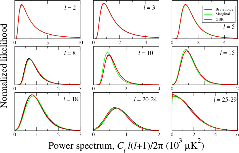
Figure 1.— Slices through the joint likelihood from a low-resolution simulation, computed by brute-force pixel space evaluation (black lines) and the Gaussianized Blackwell-Rao estimator (red lines). Green lines show the marginal distribution for each $\ell$, to illustrate the effect of mode coupling caused by the WMAP KQ85 sky cut used in this analysis.

The main problem with this approach is that one attempts to map out all possible $N$-point correlation functions between all multipoles. The number of such $N$-point functions is obviously overwhelming with increasing dimensionality. But this also hints at a possible resolution of the problem: We know by experience that the CMB likelihood is a reasonably well behaved function, in that 1) there are only weak correlations between multipoles for data sets with nearly full-sky coverage, and 2) that even including just two-point correlations (in transformed variables) produces very reasonable results (e.g., Bond, Jaffe & Knox 2000; Verde et al. 2003). This intuition will be used in the next section to define a stable likelihood estimator.

3. The Gaussianized Blackwell-Rao estimator

We now introduce a new Gibbs-based likelihood estimator we call the “Gaussianized Blackwell-Rao estimator” (GBR). The basic idea behind this approach is similar to that employed by, e.g., Bond et al. (2000) and Hamimeche & Lewis (2008), namely approximation by a multivariate Gaussian in a transformed set of variables.

Explicitly, our approximation is defined by transforming the univariate marginal distributions $P(C_{\ell}|\mathbf{d})$ into Gaussianized variables, $x_{\ell}$, and then assuming a multivariate Gaussian distribution in these transformed variables,

$$P(C_{\ell}|\mathbf{d})=\left(\prod_{\ell}\frac{\partial C_{\ell}}{\partial x_{\ell}}\right)^{-1}P(\mathbf{x}|\mathbf{d}).$$ (7)

Here $\frac{\partial C_{\ell}}{\partial x_{\ell}}$ is the Jacobian of the transformation, and $\mathbf{x}=\{x_{\ell}\}$ is a Gaussian random vector with mean $\mu=\{\mu_{\ell}\}$ and covariance matrix $\mathbf{C}_{\ell\ell^{\prime}}=\left<(x_{\ell}-\mu_{\ell})(x_{\ell^{\prime}}-\mu_{\ell^{\prime}})\right>$. Thus, the approximation of our likelihood estimator relies on the assumption that

$$P(\mathbf{x}|\mathbf{d})\approx e^{-\frac{1}{2}(\mathbf{x}-\mu)^{T}\mathbf{C}^{-1}(\mathbf{x}-\mu)}.$$ (8)

Note that this is by construction exact for the full-sky uniform noise case, because the covariance matrix in this case is diagonal, and the full expression factorizes in $\ell$; in that case we are only performing an identity operation.

3.1. Transformation to Gaussian marginal variables

The first step in our algorithm is to compute the change-of-variables rule from $C_{\ell}$ to $x_{\ell}$ that transforms the marginal distribution, $P(C_{\ell}|\mathbf{d})$, for each $\ell$ into a Gaussian distribution, $P(x_{\ell}|\mathbf{d})$. The data used for this process are the $\sigma_{\ell}$ samples drawn from the joint posterior $P(C_{\ell},\mathbf{s}|\mathbf{d})$ by the CMB Gibbs sampler.

We use two different methods of estimating the marginal distributions from these samples. The first approach is to estimate $P(C_{\ell}|\mathbf{d})$ with the Blackwell-Rao estimator as defined by Equation 5, over a grid in $C_{\ell}$ for each $\ell$. Then, a cubic spline is fitted to the resulting distribution. This is the preferred approach for high signal-to-noise or low-$\ell$ modes.

However, for low signal-to-noise and high-$\ell$ modes one observes similarly poor convergence properties of this marginal estimator as for the full joint estimator. In these cases we therefore instead compute a simple histogram directly from the $C_{\ell}$ samples, and fit a smooth spline (Green & Silverman, 1994) through this histogram. For further stability, we also produce $\mathcal{O}(10^{6})$ $C_{\ell}$ samples from $P(C_{\ell}|\sigma_{\ell})$ based on the same $\sigma_{\ell}$ set as used for the BR estimator. This essentially corresponds to computing the Blackwell-Rao estimator by Monte Carlo, and the computational cost of producing these extra samples is small. (The computational expense of the Gibbs sampler is driven by sampling from $P(\mathbf{s}|C_{\ell},\mathbf{d})$, not by $P(C_{\ell}|\mathbf{s})$.) Note that this approach naturally supports arbitrary $C_{\ell}$ binning schemes (Eriksen & Wehus, 2008), and also interfaces naturally with the hybrid MCMC scheme described by Jewell et al. (2004).

Given these spline approximations to $P(C_{\ell}|\mathbf{d})$ for each $\ell$, we compute the corresponding cumulative distributions by numerical integration,

$$F(C_{\ell}|\mathbf{d})=\int_{0}^{C_{\ell}}P(C_{\ell}^{\prime}|\mathbf{d})dC_{\ell}^{\prime}.$$

This is subsequently identified with a standard Gaussian distribution with zero mean and unity variance. Explicitly, we find $x_{\ell}(C_{\ell})$ over a grid in $C_{\ell}$ such that

$$F(C_{\ell}|\mathbf{d})=F_{\textrm{Gauss}}(x_{\ell})=\frac{1}{2}\left(1+\textrm{erf}\left(\frac{x_{\ell}}{\sqrt{2}}\right)\right),$$

where erf is the error function. This equation is straightforward to solve using standard numerical root-finding routines. The result is a convenient set of look-up tables $x_{\ell}(C_{\ell})$, again stored in the form of cubic splines, that allows for very efficient transformation from standard to Gaussian variables for arbitrary values of $C_{\ell}$. From these splines, it is also easy to compute the derivatives required for the Jacobian in Equation 7.

3.2. Estimation of the joint Gaussian density

Having defined a change-of-variables for each $\ell$, the remaining task is to estimate the joint distribution, $P(\mathbf{x}|\mathbf{d})$, in the new variables. In this paper, we approximate this distribution by a joint Gaussian, but any parametric function could of course serve this purpose. For example, we implemented support for the skew-Gaussian distribution (e.g., Azzalini & Capitanio, 2003) in our codes, but found that the improvement over a simple Gaussian was very small.

The only free parameters in this multivariate Gaussian distribution are the mean, $\mu$, and the covariance, $\mathbf{C}$. These are again estimated from the samples produced by the Gibbs sampler. First, we draw $N\sim\mathcal{O}(10^{6})$ $C_{\ell}$ samples from $P(C_{\ell}|\sigma_{\ell})$, as described above, but this time including all $\ell$’s for each sample. Then we Gaussianize these $\ell$-by-$\ell$, by evaluating $x_{\ell}(C_{\ell})$ for each sample and multipole moment. Finally, we compute the corresponding means and standard deviations,

$$\mu_{\ell} =\frac{1}{N}\sum_{i=1}^{N}x_{\ell}^{i}$$ (9)

$$C_{\ell\ell^{\prime}} =\frac{1}{N}\sum_{i=1}^{N}(x_{\ell}^{i}-\mu_{\ell})(x_{\ell^{\prime}}^{i}-\mu_{\ell^{\prime}}),$$ (10)

where the sums run over sample index.

4. Application to simulated data

Before applying the machinery described in the previous section to the 5-year WMAP data, we verify the method by a analyzing a simulated low-resolution data set. The reason for considering a low-resolution simulation is that only in this case is it possible to evaluate the exact likelihood by brute force in pixel space, without making any approximations.

The simulation is made by drawing a Gaussian realization from the best-fit 5-year WMAP $\Lambda$CDM power spectrum (Komatsu et al., 2008), smoothing this with a $10^{\circ}$ FWHM Gaussian beam, and projecting it on an $N_{\textrm{side}}=16$ HEALPix grid. Finally, $20\mu\textrm{K}$ RMS white noise is added to each pixel, and the (degraded) WMAP KQ85 sky cut (Gold et al., 2008) is applied to the data. The maximum multipole considered in this analysis was $\ell_{\textrm{max}}=47$, and the spectrum was binned with a bin size of $\Delta\ell=5$ from $\ell=20$. The signal-to-noise is unity at $\ell=19$, and negligible beyond $\ell\geq 30$.

Figure 2.— Comparison of amplitude—tilt likelihoods derived from the 5-year WMAP GBR estimator up to $\ell\leq 250$, for two independent sample sets (solid and dashed lines). Contours are where $-2\textrm{ln}\mathcal{L}(C_{\ell})$ rises by 0.1, 2.3, 6.17 and 11.8 from the minimum, corresponding to the peak and 1, 2 and $3\sigma$ confidence regions in a Gaussian distribution. See main text for full details. The cross marks the point $(q,n)=(1,0)$, corresponding to the best-fit model for WMAP including all $\ell$’s, and this is found to lie well inside the $1\sigma$ contour.

We now compute slices for each $\ell$ through the full multivariate likelihood, both with the method described in §3 and by brute-force pixel space evaluation (e.g., Eriksen et al., 2007a), fixing all other $\ell$’s at the input $\Lambda$CDM spectrum. For comparison, we also compute the the marginal distributions for each $\ell$.

The results from this exercise are shown in Figure 1. Black lines indicate the brute-force likelihoods, and red lines show the Gaussianized Blackwell-Rao likelihoods. The green lines show the marginal distributions, visualizing the effect of mode coupling due to the sky cut.

First, we see that all distributions agree very closely at $\ell\leq 8$. In this very large-scale regime, all harmonic modes are sufficiently well sampled with the KQ85 sky cut that mode coupling is negligible. However, from $\ell\geq 10$ the marginal distributions are noticeably different from the likelihood slices, with a typical shift in peak position of $\sim 100\mu\textrm{K}^{2}$’s. We also see that these correlations are accurately captured by the Gaussian approximation implemented in the GBR estimator, as the GBR likelihoods are essentially identical to the brute-force slices up to $\ell=18$.

At the very high $\ell$ and low signal-to-noise end, we see slight differences between the GBR and the pixel space slices, and in fact, the agreement is better with the marginal distributions. This is caused by poor convergence of the covariance matrix in this particular run, and is included here for pedagogical purposes only: In a real analysis, one must always make sure that all distributions have converged well, typically by analyzing different chain sets separately. Note also that with sufficiently wide bins, the correlations to neighboring bins eventually vanish, and in this case it may be better to remove these correlations by hand from the covariance matrix, rather than trying to estimate them by sampling. Whether this is the case or not for a given set can again be estimated by jack-knife tests. Finally, for the 5-year WMAP analysis presented in this paper, we will only use the GBR estimator in the high signal-to-noise regime, and in that case the distributions converge very quickly.

5. 5-year WMAP temperature analysis

We now apply the tools described in §3 to the 5-year WMAP temperature data. We only consider $\ell\leq 200$ in this paper, to avoid issues with error propagation for unresolved point sources and beam estimation. However, we do correct for the mean spectrum of unresolved point sources, as described below.

5.1. Data

We analyze the foreground reduced 5-year WMAP V-band temperature sky maps, which are available from Lambda. The V-band data was chosen because these are considered to be the cleanest in terms of foregrounds out of the five WMAP bands (Gold et al., 2008). Further, at $\ell\leq 200$ the V-band alone is strongly cosmic variance dominated, and one does therefore not gain any significant statistical power by co-adding with other bands. Instead, one only increases the chance of introducing foreground biases by adding more frequencies. We work with the individual differencing assembly (DA) maps (Hinshaw et al., 2003), and take into account the beam and noise pattern for each map separately.

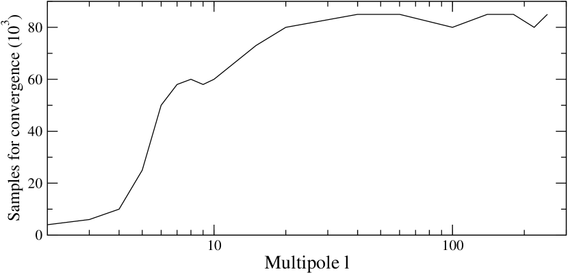
Figure 3.— Number of $C_{\ell}$ samples required for the GBR covariance matrix to converge, as a function of $\ell_{\textrm{max}}$.

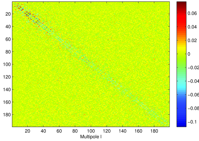
Figure 4.— GBR correlation matrix, $\tilde{\mathbf{C}}_{\ell\ell^{\prime}}$, for the 5-year WMAP V-band data.

The WMAP sky maps are pixelized at a HEALPix resolution of $N_{\textrm{side}}=512$, corresponding to a pixel size of $7^{\prime}$, and the instrumental beam of the two V-band channels has a FWHM of 21’. We therefore impose an upper harmonic mode limit of $\ell_{\textrm{max}}=700$ in the Gibbs sampling (Commander) step, probing deeply into the noise dominated regime. Note, however, that we only use $\ell\leq 200$ in the GBR estimator, to avoid high-$\ell$ complications, such as beam and point source error propagation, in the cosmological parameter stage.

We correct the spectrum for unresolved point sources using the WMAP model. Explicitly, the mean spectrum due to unresolved point sources in a single frequency, $\nu$, for the 5-year WMAP data is modelled as (Hinshaw et al., 2003, 2007; Nolta et al., 2008)

$$C_{\ell}^{\textrm{ps}}=A_{\textrm{ps}}a(\nu)^{2}\left(\frac{\nu}{\nu_{0}}\right)^{2\beta},$$ (11)

where $A_{\textrm{ps}}=0.011\pm 0.001$ is the point source amplitude relative to the Q-band channel ($\nu_{0}=41\textrm{GHz}$), $\beta=-2.1$ is the best-fit spectral index of the point sources, and $a(\nu)$ is the conversion factor between antenna and thermodynamic temperature units. To correct for this in our analysis, we subtract $C_{\ell}^{\textrm{ps}}$, evaluated at $\nu=61\textrm{GHz}$, from each $\sigma_{\ell}$ sample before computing the GBR estimator.

Finally, we impose the WMAP KQ85 sky cut (Gold et al., 2008) on the data that masks point sources, removing 18% of the sky. Note that we adopt the template corrected maps provided by the WMAP team in this analysis, and postpone an internal Gibbs sampling based foreground analysis to a future paper; for now our main focus is the new likelihood approximation, not the impact of foregrounds.

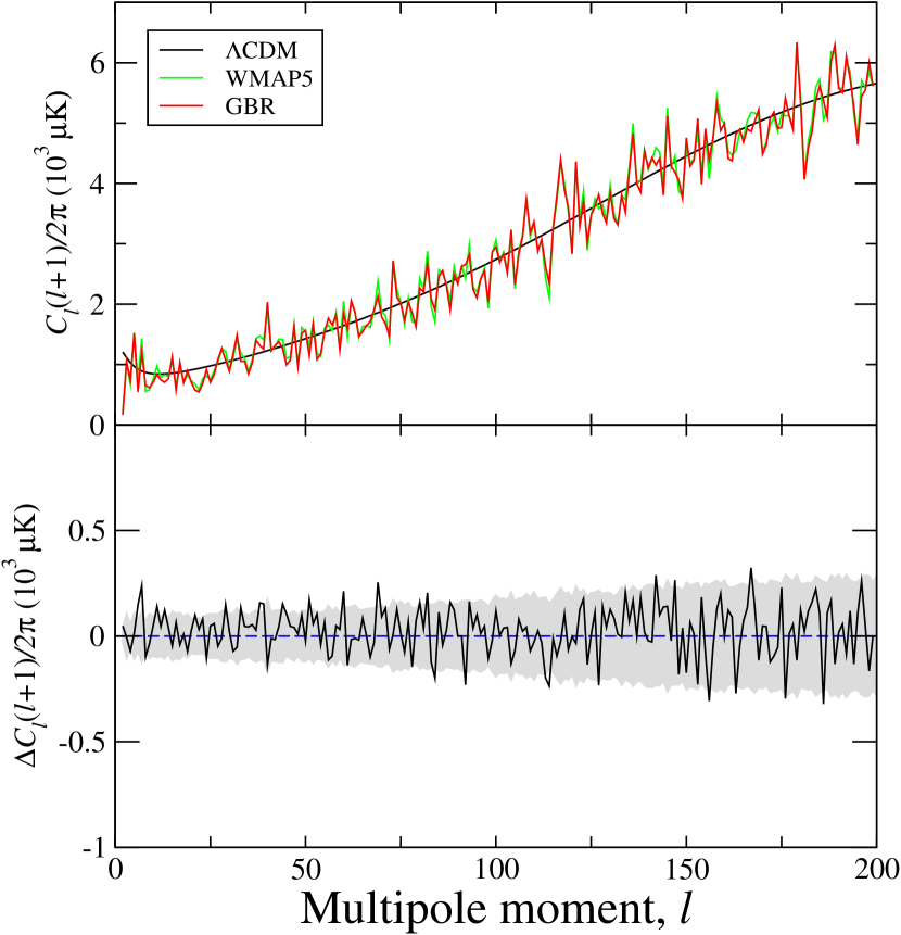
Figure 5.— Comparison of 5-year power spectra obtained by WMAP and Commander/GBR up to $\ell=200$. The bottom panel shows the difference of these two spectra, and the gray band indicates the 68% confidence region due to noise and sky cut only, not cosmic variance.

5.2. Analysis overview

The analysis consists of the following steps:

1. Generate 4000 $\sigma_{\ell}$ samples with Commander from the 5-year V1 and V2 differencing assemblies , including $\ell$’s up to $\ell_{\textrm{max}}=700$, divided over 8 chains.

2. Generate 500 000 $C_{\ell}$ samples from these $\sigma_{\ell}$’s, including $\ell$’s between $\ell=2$ and 250.

3. Compute the corresponding GBR parameters, i.e., transformation tables, means $\mu$ and covariance matrix $\mathbf{C}$.

4. Modify the 5-year WMAP temperature likelihood by replacing the existing low-$\ell$ part with Equation 7, with the parameters given in (3). The transition multipole between the low-$\ell$ and high-$\ell$ is increased from $\ell=32$ to 200. Multipoles between $\ell=201$ and 250 are included in the GBR estimator to avoid truncation effects, but the spectrum in this range is kept fixed at a fiducial spectrum, in order not to count these multipoles twice.

5. Cosmological parameters are estimated using CosmoMC (Lewis & Bridle, 2002).

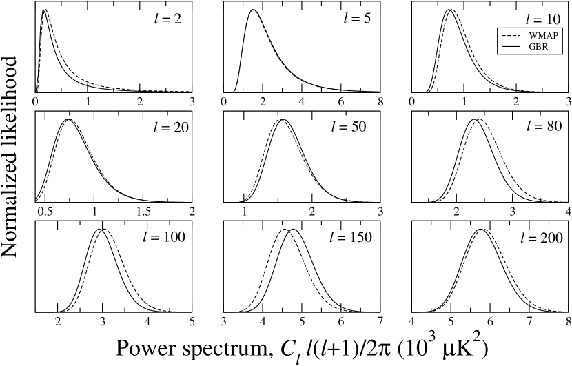
Figure 6.— Comparison of likelihood slices from the standard WMAP likelihood code (dashed lines) and the new GBR likelihood (solid lines).

5.3. Convergence analysis

Before presenting the results from the WMAP analysis, we consider the question of convergence. First, we compute the Gelman-Rubin statistic (Gelman & Rubin, 1992) for each $\sigma_{\ell}$ using the eight chains computed with Commander and removing the first 20 samples for burn-in. We find that $R-1$ is less than 0.01 for $\ell\lesssim 300$ and less than 1.1 for $\ell\lesssim 500$, indicating very good convergence in terms of power spectra.

However, the fact that each $\sigma_{\ell}$ individually is well converged does not automatically imply that the full likelihood is well converged, since the latter depends crucially on the correlations between $\sigma_{\ell}$’s. To assess the convergence in terms of cosmological parameters, we therefore analyse a toy model, by fitting a simple two-parameter amplitude and tilt, $q$ and $n$, model,

$$C_{\ell}=q\,\left(\frac{\ell}{\ell_{\textrm{pivot}}}\right)^{n}\,C_{\ell}^{\textrm{fid}},$$ (12)

to the WMAP data between $\ell=2$ and 250 with the GBR likelihood. Here $C_{\ell}^{\textrm{fid}}$ is a fiducial power spectrum, which is chosen to be the best-fit 5-year WMAP $\Lambda$CDM power spectrum (Komatsu et al., 2008), and $\ell_{\textrm{pivot}}=150$. We then map out the likelihood in a grid over $q$ and $n$. This is repeated twice, first including samples from chains number 1 to 4 and then from chains number 5 to 8.

The results from this exercise are shown in Figure 2 in terms of two sets of likelihood contours, corresponding to each of the two chain sets, respectively. The agreement between the two is excellent, indicating that we also have good convergence in terms of cosmological parameters with the existing sample set. Note also that the point $(q,n)=(1,0)$ lies well inside the $1\sigma$ confidence region, indicating that the best-fit WMAP model, which is obtained including $\ell$’s between $\ell=2$ and 1024, also is a good fit to $\ell=2$ to 250 separately.

Third, as described in §3, we construct the GBR covariance matrix from $N=\mathcal{O}(10^{6})$ $C_{\ell}$ samples drawn from the (smaller) set of $\sigma_{\ell}$ samples. An outstanding question is how large $N$ should be in order for this covariance matrix to reach convergence, as a function of $\ell_{\textrm{max}}$. To settle this question, we carry out the following simple exercise: First we produce two $C_{\ell}$ sample sets, each containing $N$ samples, and all drawn from a single $\sigma_{\ell}$ sample. Second, we compute the two corresponding covariance matrices, invert these, then subtract them from each other, and finally compute the standard deviation of all elements. Third, we define the inverse covariance matrix to be converged if the RMS MCMC noise is less than 0.005, corresponding to 0.5% of the diagonal elements. (We have checked that this produces robust parameter estimates.) We then find the smallest $N$ such that this is satisfied, as a function of $\ell_{\textrm{max}}$.

The results from this exercise are shown in Figure 3. Here we see that the number of samples required for convergence rises rapidly up to $\ell\sim 30$, reaching a maximum of $\sim 8\times 10^{4}$ samples, and then flattens to a plateau. To be on the safe side, we therefore always use either $5\times 10^{5}$ or $10^{6}$ samples in the WMAP analysis.

The reason for this behaviour becomes intuitive when considering the structure of the actual matrix. This is shown in Figure 4, on the form of a correlation matrix

$$\tilde{C}_{\ell\ell^{\prime}}=\frac{C_{\ell\ell^{\prime}}}{\sqrt{C_{\ell\ell}C_{\ell^{\prime}\ell^{\prime}}}}-\delta_{\ell\ell^{\prime}}.$$ (13)

The main features of this matrix are negative correlations around the diagonal, with the largest amplitudes observed between $\ell$ and $\ell\pm 2$. This is expected: First, two modes separated by $\Delta\ell=1$ have different parity, and can therefore not easily mimic each other. On the other hand, modes separated by $\Delta\ell=2$ have both identical parity and similar angular scale, and it is therefore possible to add power to one mode and subtract it from the other, and still maintain an essentially unchanged image. The result is a noticeable anti-correlation between $\ell$ and $\ell\pm 2$.

At larger separations in $\ell$, the correlations die off rapidly, since it is difficult for a large-scale mode to mimic a small-scale mode with a reasonably small sky cut. And this explains the convergence behaviour seen in Figure 3: The covariance matrix is strongly band-limited. Therefore, once one has a sufficiently large number of $C_{\ell}$ samples for a sub-block to converge, there is also enough samples for a sub-block further away to converge. These are essentially uncorrelated.

5.4. Results

We now present the main results derived from the 5-year WMAP temperature data with the GBR estimator between $\ell=2$ and 200. First, in the top panel of Figure 5 we plot the power spectrum obtained by maximizing the GBR likelihood together with the official 5-year WMAP power spectrum. The bottom panel shows the difference between these two, and the gray band indicates the standard deviation of $\sigma_{\ell}$, i.e., the uncertainty due to noise and sky cut, but not to cosmic variance. Clearly, the agreement between the two power spectra is very good.

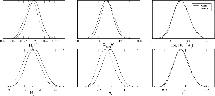
Figure 7.— Comparison of marginal cosmological parameter posteriors obtained with the standard WMAP likelihood code (dashed lines) and with the modified GBR likelihood code up to $\ell=200$ (solid line) for 5-year WMAP data.

Next, in Figure 6 we compare a few selected slices through the GBR likelihood with slices through the WMAP likelihood. All other $\ell$’s than the one currently considered are kept fixed at the best-fit $\Lambda$CDM spectrum. Here we see that there are small shifts in peak positions, corresponding to the small differences seen in the power spectra in Figure 5. However, a main point in this plot is that the GBR likelihood slices are well behaved even at the highest $\ell$’s, and this is not the case for the standard BR estimator (Chu et al., 2005).

Finally, in Table 1 and Figure 7 we summarize the marginal cosmological parameter posteriors obtained with the two likelihood codes from CosmoMC. Interestingly, there are some notable differences at the 0.3–$0.6\sigma$ level, with the most striking example being the spectral index of scalar perturbations, $n_{\textrm{s}}=0.973\pm 0.014$. This is only $1.9\sigma$ away from unity, and $0.6\sigma$ higher than the official WMAP values.

6. Conclusions

We have presented a new likelihood approximation to be used within the CMB Gibbs sampling framework. This approximation is defined by Gaussianizing the observed marginal power spectrum posteriors, $P(C_{\ell}|\mathbf{d})$, through a specific change-of-variables, and then coupling these univariate posteriors into a joint distribution through a multivariate Gaussian in the new variables. This process is exact, i.e., an identity operation, in the uniform and full-sky coverage case, and it is also an excellent approximation in for the moderate sky cuts relevant to satellite missions such as WMAP and Planck.

Our new approach relies on the previously described CMB Gibbs sampling framework (Jewell et al., 2004; Wandelt et al., 2004; Eriksen et al., 2004), and thereby inherits many important advantages from that. First and foremost, this framework allows for seamless propagation of uncertainties from various systematic effects (e.g., foregrounds, beam uncertainties, calibration or noise estimation errors) to the final cosmological parameters. This is not straightforward in the hybrid scheme used by the WMAP code. Second, this new approach corresponds to the exact low-$\ell$ pixel space likelihood part of the WMAP code, not the approximate high-$\ell$ MASTER part. Still, our method can handle arbitrary high $\ell$’s. Third, once the one-time pre-processing step has been completed, the computational expense of our estimator is determined by the cost of $\ell_{\textrm{max}}$ spline evaluations, while a pixel space approach requires a matrix inversion, and therefore scales as $\mathcal{O}(N_{\textrm{pix}}^{3})$. For the cases considered in this paper, the CPU time required for the GBR WMAP estimator up to $\ell=200$ was $\sim 0.2$ milliseconds, while it was $\sim 20$ seconds for the pixel space approach up to $\ell=32$, for a map with $~{}2500$ pixels.

In order to validate our estimator, we applied it to a low-resolution simulated data set, and compared it to slices through the exact joint likelihood as computed by brute-force evaluation in pixel space. The agreement between the two approaches was excellent. We then applied the same estimator to the 5-year WMAP temperature data, and estimated both a new power spectrum and new cosmological parameters within a standard six-parameter $\Lambda$CDM model.

The results from these calculations are interesting. First, our power spectrum is statistically very similar to the official WMAP spectrum, with no visible biases seen and relative fluctuations within the level predicted by noise and sky cut. Nevertheless, we do find significant differences in terms of cosmological parameters, and most notably in the spectral index of scalar perturbations, $n_{\textrm{s}}$. Specifically, we find $n_{\textrm{s}}=0.973\pm 0.014$, which is only $1.9\sigma$ away from unity and $0.6\sigma$ higher than the official WMAP result, $n_{\textrm{s}}=0.965\pm 0.014$.

This result resembles very much the outcome of a re-analysis we did with the 3-year WMAP temperature data (Eriksen et al., 2007a), for which we found a bias of $0.4\sigma$ in $n_{\textrm{s}}$ compared to the official WMAP results. This bias was due to the sub-optimal MASTER-based likelihood approximation (Hivon et al., 2002; Verde et al., 2003) used by the WMAP team between $\ell=12$ and 30, whereas we used an exact estimator in the same range. This study later prompted the WMAP to change their codes to use an exact likelihood evaluator up to $\ell=30$.

In the same study, we also tried to increase the $\ell$-range for our exact estimator to $\ell=50$, but found small differences. We therefore concluded, perhaps somewhat prematurely, that an exact estimator up to $\ell=30$ was sufficient for obtaining accurate results. On the contrary, in this paper we find still find significant changes when increasing the exact estimator up to $\ell=200$.

In retrospect, this should perhaps not come as a complete surprise, when realizing that the impact on a particular cosmological parameter typically depends logarithmically on $\ell$. For instance, Hamimeche & Lewis (2008) considered a simple power spectrum model with a single free amplitude, $C_{\ell}=q\,C_{\ell}^{\textrm{fid}}$, and found that, for a given likelihood estimator to be “statistically unbiased”, the systematic errors in that same estimator must fall off faster than $\sim 1/\ell$.

Table 1Marginal 5-year WMAP cosmological parameters

Parameter	WMAP	GBR	Shift in $\sigma$
$\Omega_{\textrm{b}}h^{2}$	$0.0228\pm 0.0006$	$0.0230\pm 0.0006$	0.4
$\Omega_{\textrm{c}}h^{2}$	$0.109\pm 0.006$	$0.0108\pm 0.006$	-0.3
$\textrm{log}(10^{10}A_{\textrm{s}})$	$3.06\pm 0.04$	$3.06\pm 0.04$	0.0
$h$	$0.722\pm 0.03$	$0.732\pm 0.03$	0.3
$n_{\textrm{s}}$	$0.965\pm 0.014$	$0.973\pm 0.014$	0.6
$\tau$	$0.090\pm 0.02$	$0.090\pm 0.02$	0.0

Note. — Comparison of cosmological parameters obtained with the standard 5-year WMAP likelihood code (second column) and with the new GBR estimator at $\ell\leq 200$ (third column), given in terms of marginal means and standard deviations. The shift between the two in units of $\sigma$ is listed in the fourth column.

A similar consideration holds for $n_{\textrm{s}}$. Intuitively, $n_{\textrm{s}}$ is as much affected by $\ell=2$ to 10 as it is between $\ell=20$ and 100. In the previous 3-year WMAP re-analysis paper, we increased the range of the accurate likelihood estimator from $\ell=12$ to 30, corresponding to a factor of 2.5 in $\ell$, and removed a bias of $\sim 0.4\sigma$ in $n_{\textrm{s}}$. In this paper, we increase the range from $\ell=30$ to 200, corresponding to a factor of 6.7 in $\ell$, and find an additional bias of $0.6\sigma$. However, increasing $\ell$ from 30 to 50 corresponds only to a factor of 1.7 in $\ell$, and this appears to be too small to produce a statistically significant result.

The main conclusions from this work are two-fold. First, it seems that an accurate likelihood description is required to higher $\ell$’s than previously believed, and at least up to $\ell=200$, in order to obtain unbiased results. By extrapolation, it also does not seem unlikely that even higher multipoles should be included. This issue will be revisited in a future publication.

Our second main conclusion is that we find a spectral index only $1.9\sigma$ away from unity, namely $n_{\textrm{s}}=0.973\pm 0.014$. To us, it therefore seem premature to make strong claims concerning $n_{\textrm{s}}\neq 1$; the statistical significance of this is rather low, and there are likely still unknown systematic errors in this number.

In a future publication we will generalize the GBR estimator to polarization. Once completed, this will enable a fully Gibbs-based CMB likelihood analysis at low $\ell$’s, and remove the need for likelihood techniques based on matrix operations, i.e., inversion and determinant evaluation. The computational cost of a standard cosmological parameter MCMC analysis (e.g., CosmoMC) will then once again be driven by the required Boltzmann codes (e.g., CAMB or CMBFast) and not by the likelihood evaluation. In turn, this will increase the importance of fast interpolation codes such as Pico (Fendt & Wandelt, 2007) or COSMONET (Auld et al., 2007). With such fast algorithms for both spectrum and likelihood evaluations ready at hand, the CPU requirements for cosmological parameter estimation may possibly be reduced by orders of magnitude.

References

- Auld et al. (2007) Auld, T., Bridges, M., Hobson, M. P., & Gull, S. F. 2007, MNRAS, 376, L11
- Azzalini & Capitanio (2003) Azzalini, A. & Capitanio, A. 2003, J.Roy.Statist.Soc, series B, vol.65, pp.367-389
- Bennett et al. (2003) Bennett, C. L., et al. 2003, ApJS, 148, 1
- Bond et al. (2000) Bond, J. R., Jaffe, A. H., & Knox, L. 2000, ApJ, 533, 19
- Chu et al. (2005) Chu, M., Eriksen, H. K., Knox, L., Górski, K. M., Jewell, J. B., Larson, D. L., O’Dwyer, I. J., & Wandelt, B. D. 2005, Phys. Rev. D, 71, 103002
- Eriksen et al. (2004) Eriksen, H. K., et al. 2004, ApJS, 155, 227
- Eriksen et al. (2007a) Eriksen, H. K., et al. 2007a, ApJ, 656, 641
- Eriksen et al. (2007b) Eriksen, H. K., Huey, G., Banday, A. J., Górski, K. M., Jewell, J. B., O’Dwyer, I. J., & Wandelt, B. D. 2007b, ApJ, 665, L1
- Eriksen et al. (2008a) Eriksen, H. K., Jewell, J. B., Dickinson, C., Banday, A. J., Górski, K. M., & Lawrence, C. R. 2008a, ApJ, 676, 10
- Eriksen et al. (2008b) Eriksen, H. K., Dickinson, C., Jewell, J. B., Banday, A. J., Górski, K. M., & Lawrence, C. R. 2008b, ApJ, 672, L87
- Eriksen & Wehus (2008) Eriksen, H. K. & Wehus, I. K. 2008, ApJS, in press, [arxiv:0806.3074]
- Fendt & Wandelt (2007) Fendt, W. A., & Wandelt, B. D. 2007, ApJ, 654, 2
- Gelfand & Smith (1990) Gelfand, A. E., & Smith, A. F. M. 1990, J. Am. Stat. Asso., 85, 398
- Gelman & Rubin (1992) Gelman, A., & Rubin, D. 1992, Stat. Sci., 7, 457
- Gold et al. (2008) Gold, B., et al. 2008, ApJS, [arXiv:0803.0715]
- Górski et al. (2005) Górski, K. M., Hivon, E., Banday, A. J., Wandelt, B. D., Hansen, F. K., Reinecke, M., & Bartelmann, M. 2005, ApJ, 622, 759
- Green & Silverman (1994) Green, P. J., & Silverman, B. W. 1994, Non-Parametric Regression and Generalized Linear Models, Chapman and Hall, 1994
- Groeneboom & Eriksen (2008) Groeneboom, N. E., & Eriksen, H. K. 2008, ApJ, in press, [arXiv:0807.2242]
- Hamimeche & Lewis (2008) Hamimeche, S., & Lewis, A. 2008, Phys. Rev. D, 77, 103013
- Hinshaw et al. (2003) Hinshaw, G., et al. 2003, ApJS, 148, 63
- Hinshaw et al. (2007) Hinshaw, G., et al. 2007, ApJS, 170, 288
- Hinshaw et al. (2008) Hinshaw, G., et al. 2008, ApJS, in press, [arXiv:0803.0732]
- Hivon et al. (2002) Hivon, E., Górski, K. M., Netterfield, C. B., Crill, B. P.,Prunet, S., & Hansen, F. 2002, ApJ, 567, 2
- Jewell et al. (2004) Jewell, J., Levin, S., & Anderson, C. H. 2004, ApJ, 609, 1
- Jewell et al. (2008) Jewell, J. B., et al. 2008, submitted, ApJ, [astro-ph/0807.0624]
- Komatsu et al. (2008) Komatsu, E., et al. 2008, ApJS, in press, [arXiv:0803.0547]
- Larson et al. (2007) Larson, D. L., Eriksen, H. K., Wandelt, B. D., Górski, K. M., Huey, G., Jewell, J. B., & O’Dwyer, I. J. 2007, ApJ, 656, 653
- Lewis & Bridle (2002) Lewis, A., & Bridle, S. 2002, Phys. Rev. D, 66, 103511
- Nolta et al. (2008) Nolta, M. R., et al. 2008, ApJS, in press, [arXiv:0803.0593]
- O’Dwyer et al. (2004) O’Dwyer, I. J., et al. 2004, ApJ, 617, L99
- Verde et al. (2003) Verde, L., et al. 2003, ApJS, 148, 195
- Wandelt et al. (2004) Wandelt, B. D., Larson, D. L., & Lakshminarayanan, A. 2004, Phys. Rev. D, 70, 083511