The effects of twisted magnetic field on coronal loops oscillations and dissipation

Abstract

The standing MHD modes in a zero-$\beta$ cylindrical magnetic flux tube modelled as a straight core surrounded by a magnetically twisted annulus, both embedded in a straight ambient external field is considered. The dispersion relation for the fast MHD waves is derived and solved numerically to obtain the frequencies of both the kink ($m=1$), and fluting ($m=2,3$) waves. Damping rates due to both viscous and resistive dissipations in presence of the twisted magnetic field is derived and solved numerically for both the kink and fluting waves.

Key words.   Sun: corona – Sun: magnetic fields – Sun: oscillations

1 Introduction

Solar corona is a highly structure of magnetic flux tubes namely coronal loops. Transverse oscillations of coronal loops were first identified by Aschwanden et al. (1999) and Nakariakov et al. (1999) using the observations of TRACE. Edwin & Roberts (1983) elaborated on the dispersion relation for a magnetic cylinder embedded in a magnetic environment typical of that of the solar photosphere and corona. They found that the existence of inhomogeneities in the form of structuring of the magnetic field enables loops to act as wave guides for a variety of different modes. Karami, Nasiri $\&$ Sobouti (2002) used the model of Edwin & Roberts (1983) but without limiting it to slender tubes. They solved numerically the dispersion relation for each mode in its full generality. They obtained that in presence of weak viscous and ohmic dissipations, the damping rate is inversely proportional to the Reynolds and Lundquist numbers, R and S, respectively.

An additional features of the flux tube is that of twist. Bennett, Roberts $\&$ Narain (1999) examined the influence of magnetic twist on the modes of oscillations of a magnetic flux tube. They found that twist introduces an infinite band of body modes. Klimchuk, Antiochos $\&$ Norton (2000) introduced twist to resolve the internal structure on an individual loop embedded within a much larger dipole configuration. Mikhalyaev $\&$ Solov’ev (2005) investigated the MHD waves in a double magnetic flux tube embedded in a uniform external magnetic field. The tube consists of a dense hot cylindrical cord surrounded by a co-axial shell. They found two slow and two fast magnetosonic modes can exist in the thin double tube.

Verwichte et al. (2004), using the observations of TRACE, detected the multimode oscillations for the first time. They found that two loops are oscillating in both the fundamental and the first-overtone standing fast kink modes. According to the theory of MHD waves, for uniform loops the period ratio $P_{1}/2P_{2}$ of the fundamental mode and its first overtone is exactly 1. But the ratios found by Verwichte et al. (2004) are 0.91$\pm$0.04 and 0.79$\pm$0.03 and thus clearly differ from 1. This may be caused by different factors such as the effects of curvature, see e.g. Van Doorsselaere et al. (2004), leakage, see De Pontieu et al. (2001), density stratification in the loops, see e.g. Andries et al. (2005), Erdelyi & Verth (2007), Karami & Asvar (2007) and magnetic twist, see Erdélyi & Fedun (2006) and Erdélyi & Carter (2006).

Erdélyi & Fedun (2006), studied the wave propagation in twisted cylindrical magnetic flux tube embedded in an incompressible but also magnetically twisted plasma. They found that magnetic twist will increase, in general, the periods of waves approximately by a few percent when compare to their untwisted counterparts. Erdélyi & Carter (2006) used the model of Mikhalyaev & Solov’ev (2005) but for a fully magnetically twisted configuration consisting of a core, annulus and external region. They investigated their analysis by considering magnetic twist just in the annulus, the internal and external regions having straight magnetic field. Two modes of oscillations occurred in this configurations; surface and hybrid modes. They found that when the magnetic twist is increase the hybrid modes cover a wide range of phase speeds, centered around the annulus, longitudinal Alfvén speed for the sausage modes.

Carter & Erdélyi (2007) investigated the oscillations of a magnetic flux tube configuration consisting of a core, annulus and external region each with straight distinct magnetic field in an incompressible medium. They found that there are two surface modes arising for both the sausage and kink modes for the annulus-core model where the monolithic tube has solely one surface mode for the incompressible case. Also they showed that the existence and width of an annulus layer has an effect on the phase speeds and periods. Carter & Erdélyi (2008) used the model introduced by Erdélyi & Carter (2006) to include the kink modes. They found for the set of kink body modes, the twist increase the phase speeds of the modes. Also they showed that there are two surface modes for the twisted shell configuration, one due to each surface, where one mode is trapped by the inner tube, the other by the annulus itself.

In the present work, our aim is to investigate the effects of the twisted magnetic field on oscillations and damping of standing MHD waves in the cold coronal loops observed by Verwichte et al. (2004) deduced from the TRACE data. This paper is organized as follows. In Section 2 we use the model introduced by Erdélyi & Carter (2006) to derive the equations of motion, introduce the relevant boundary conditions and obtain the dispersion relation. In Section 3 we discuss resistive and viscous dissipations to calculate contributions of the different modes to heating of the coronal loops. In Section 4 we give numerical results. Section 5 is devoted to conclusions.

2 Equations of Motion

The linearized MHD equations for a zero-$\beta$ incompressible plasma are

$$\frac{\partial\delta\mathbf{v}}{\partial t}=\frac{1}{4\pi\rho}\{(\nabla\times\delta\mathbf{B})\times\mathbf{B}+(\nabla\times\mathbf{B})\times\delta\mathbf{B}\}+\frac{\eta}{\rho}\nabla^{2}\delta\mathbf{v},$$ (1)

$$\frac{\partial\delta\mathbf{B}}{\partial t}=\nabla\times(\delta\mathbf{v}\times\mathbf{B})+\frac{c^{2}}{4\pi\sigma}\nabla^{2}\delta\mathbf{B},$$ (2)

$$P_{\rm T}=\frac{\mathbf{B}\cdot\delta\mathbf{B}}{4\pi},$$ (3)

$$\nabla\cdot\delta\mathbf{v}=0,$$ (4)

where $\delta\bf{v}$, $\delta\bf{B}$ and $P_{\rm T}$ are the Eulerian perturbations in the velocity, magnetic field and magnetic pressure, respectively; $\rho$, $\sigma$, $\eta$ and $c$ are the mass density, the electrical conductivity, the viscosity and the speed of light, respectively. Note that Eq. (4) satisfies the incompressibility condition.

The simplifying assumptions are:

• $\rho$ is constant over the loop;

• for a zero-$\beta$ loop, gas pressure is negligible;

• from Erdélyi $\&$ Carter (2006), background magnetic field is assumed to be

  $${\mathbf{B}}=\left\{\begin{array}[]{lll}{\mathbf{B}}_{i}=(0,0,B_{i}),~{}~{}~{}~{}~{}~{}~{}r<a,\\ {\mathbf{B}}_{0}=(0,A_{0}r,B_{0}),~{}~{}~{}a<r<R,\\ {\mathbf{B}}_{e}=(0,0,B_{e}),~{}~{}~{}~{}~{}~{}~{}r>R,\\ \end{array}\right.$$

  where $A_{0}$, $B_{i}$, $B_{0}$, $B_{e}$ are constant and $a$, $R$ are radii of the core and tube, respectively;

• tube geometry is a circular with cylindrical coordinates, ($r,\phi,z$);

• there is no initial steady flow over the tube;

• viscous and resistive coefficients, $\eta$ and $\sigma$ respectively, are constants;

• t-, $\phi$- and z- dependence for any of the components $\delta{\bf{v}}$ and $\delta{\bf{B}}$ is $\exp{\{i(m\phi+k_{z}z-\omega t)\}}$. Where $k_{z}=l\pi/L$, $L$ is length of the tube, and $l=(1,2,\cdot\cdot\cdot)$, $m=(0,1,2,\cdot\cdot\cdot)$ are the longitudinal and azimuthal mode numbers, respectively.

We will further assume that the dissipative terms in Eqs. (1) and (2) are much smaller. We will first solve the problem without these terms and re-introduce them later as small corrections in calculating contributions of the different modes to heating of the corona. Taking time derivative of Eq. (2) and substituting for $\partial\delta{\mathbf{v}}/\partial t$ from Eq. (1), the resulting equation yields to Bessel’s equation

$$\frac{d^{2}{P_{\rm T}}}{dr^{2}}+\frac{1}{r}\frac{d{P_{\rm T}}}{dr}-\Big{(}\frac{m^{2}}{r^{2}}+m_{0}^{2}\Big{)}{P_{\rm T}}=0,$$ (5)

where

$$m_{0}^{2}=k_{z}^{2}\Big{[}1-\frac{{A_{0}^{2}}{\omega_{A_{0}}^{2}}}{\pi\rho_{0}({\omega^{2}}-{\omega_{A_{0}}^{2}})^{2}}\Big{]},$$ (6)

and

$${\omega_{A_{0}}}=\frac{1}{\sqrt{4\pi\rho_{0}}}(mA_{0}+k_{z}B_{0}).$$ (7)

Equation (5) is same as the result exactly derived by Erdélyi $\&$ Carter (2006). Note that subscripts 0 (which correspond to annulus) are replaced by $i$, $e$ corresponding to the internal and external regions, respectively. Since for the internal and external regions $A_{i}$=$A_{e}$=0, hence $m_{i}^{2}=m_{e}^{2}=k_{z}^{2}>0$ and ${\omega_{A_{i}}}=\frac{k_{z}B_{i}}{\sqrt{4\pi\rho_{i}}}$, ${\omega_{A_{e}}}=\frac{k_{z}B_{e}}{\sqrt{4\pi\rho_{e}}}$.

Solutions of Eq. (5) are:

$$P_{\rm T}=\alpha I_{m}{(k_{z}r)},$$ (8)

for the interior region ($r<a$),

$$P_{\rm T}=\Big{\{}\begin{array}[]{ll}\beta I_{m}(m_{0}r)+\gamma K_{m}(m_{0}r),~{}~{}m_{0}^{2}>0,\\ \beta J_{m}(n_{0}r)+\gamma Y_{m}(n_{0}r),~{}~{}~{}~{}~{}n_{0}^{2}=-m_{0}^{2}>0,\\ \end{array}$$ (11)

for the annulus region ($a<r<R$) and

$$P_{\rm T}=\delta K_{m}{(k_{z}r)},$$ (12)

for the exterior region ($r>R$). Where ($J_{m},Y_{m}$) and ($I_{m},K_{m}$) are the Bessel and modified Bessel functions of the first and second kind, respectively. The coefficients $\alpha,\beta,\gamma$ and $\delta$ are determined by the boundary conditions. From both Karami, Nasiri $\&$ Sobouti (2002) and Erdélyi & Carter (2006), the necessary boundary conditions are that: at the boundaries $r=a$ and $r=R$, both the Lagrangian magnetic pressure and $\delta v_{r}$ should be continuous. These conditions yield to the dispersion relations for surface, $m_{0}^{2}>0$, and hybrid, $m_{0}^{2}<0$, modes which are same as the results obtained by Erdélyi & Carter (2006) in Eqs. (28a) to (28b), respectively. Note that numerical solution of the dispersion relation yields to eigenfrequencies, which are characterized by a trio of wave numbers ($n,m,l$) that actually count the number of nodes or antinodes along $r,~{}\phi$, and $z$ directions, respectively.

3 Dissipative Processes

Since the discovery of the hot solar corona about 66 years ago, different theories of coronal heating have been put forward and debated. For instance, Nakariakov et al. (1999) reported the detection of spatial oscillations in five coronal loops with periods ranging from 258 to 320 s. The decay time was $(14.5\pm 2.7)$ minutes for an oscillation of $(3.9\pm 0.13)$ millihertz. Also Wang & Solanki (2004) described a loop oscillation observed on 17 April 2002 by TRACE in 195${\AA}$. They interpreted the observed loop motion as a vertical oscillation, with a period of 3.9 minutes and a decay time of 11.9 minutes. All these observations indicate strong dissipation of the wave energy that may be the cause of coronal heating.

Following Karami & Asvar (2007), the finite conductivity and viscosity of plasma causes an exponential time decay of disturbances. Hence for weak dissipations one may assume

$$\delta{{\mathbf{B}}}^{\rm dissipative} = \delta{\mathbf{B}}({\mathbf{r}})e^{-(i\omega+\alpha)t},$$

$$\delta{{\mathbf{v}}}^{\rm dissipative} = \delta{{\mathbf{v}}}({\mathbf{r}})e^{-(i\omega+\alpha)t},$$ (13)

where $\omega$, $\delta{\bf{B}}$, and $\delta{\bf{v}}$ on the right hand side are the solutions of Eqs. (1), (2) in the absence of dissipations. Substituting Eq. (13) in Eqs. (1) and (2), canceling out the non dissipative terms, and keeping only the first order terms in $\alpha$, $c^{2}/4\pi\sigma$ and $\eta$ gives

$$2i\alpha\omega\delta{\mathbf{B}} = \frac{c^{2}}{4\pi\sigma}\Big{\{}\nabla^{2}[(\mathbf{B}\cdot\nabla)\delta\mathbf{v}]-\nabla^{2}[(\delta\mathbf{v}\cdot\nabla)\mathbf{B}]\Big{\}}$$ (14)

$$+ \frac{\eta}{\rho}\Big{\{}(\mathbf{B}\cdot\nabla)\nabla^{2}\delta\mathbf{v}-(\nabla^{2}\delta\mathbf{v}\cdot\nabla)\mathbf{B}\Big{\}},$$

where

$$\delta\mathbf{v} = -\frac{i}{4\pi\rho}\frac{\omega}{(\omega^{2}-\omega_{A}^{2})}\Big{\{}\mathbf{\nabla}(\mathbf{B}\cdot\delta\mathbf{B})-(\delta\mathbf{B}\cdot\mathbf{\nabla})\mathbf{B}\Big{\}}.$$ (15)

Rewriting Eq. (14) for either the transverse or the z-component and substituting for all quantities in terms of $\delta{B}_{z}$ gives

$$\alpha = \Big{(}\frac{k_{z}^{2}-m_{0}^{2}}{2}\Big{)}\Big{[}\frac{c^{2}}{4\pi\sigma}+\frac{\eta}{\rho_{0}}\Big{]},$$ (16)

$$= \frac{v_{A_{i}}{\rm R}}{\rho_{0}}\Big{(}\frac{\omega_{A_{0}}k_{z}A_{0}}{2\pi(\omega^{2}-\omega_{A_{0}}^{2})}\Big{)}^{2}\Big{[}\frac{1}{S}+\frac{1}{\mathcal{R}}\Big{]},$$

where $v_{A_{i}}=\frac{B_{i}}{\sqrt{4\pi\rho_{i}}}$, the Lundquist number $S=\Big{(}\frac{4\pi\sigma{\rm R}^{2}}{c^{2}}\Big{)}/\Big{(}\frac{2\pi{\rm R}}{v_{A_{i}}}\Big{)}$, is the ratio of the resistive time scale to the Alfvén crossing time and the Reynolds number ${\mathcal{R}}=\Big{(}\frac{{\rm R}^{2}\rho_{0}}{\eta}\Big{)}/\Big{(}\frac{2\pi{\rm R}}{v_{A_{i}}}\Big{)}$ is the ratio of the viscous time scale to the Alfvén crossing time. Equation (16) shows that when the twist is absent, $A_{0}=0$, the damping rate is vanished. Whereas for compressible plasma it is not zero. See Karami, Nasiri $\&$ Sobouti (2002).

4 Numerical Results

As typical parameters for a coronal loop, we assume $L=109\times 10^{3}$ km, ${\rm R/L}=0.01$, $\rho_{e}/\rho_{i}=0.1$, $\rho_{0}/\rho_{i}=0.5$, $\rho_{i}=2\times 10^{-14}$ gr cm^-3, $B_{e}/B_{i}=1$, $B_{0}/B_{i}=1$, $B_{i}=100$ G. For such a loop one finds $v_{A_{i}}=2000$ km s^-1, $\omega_{A_{\rm i}}:=\frac{v_{A_{i}}}{{\rm R}}=1.835$ rad s^-1. We use $S=10^{4}$ and ${\mathcal{R}}=560$, given by Ofman et al. (1994).

The effects of twisted magnetic field on both the frequencies $\omega$ and damping rates $\alpha$ are calculated by numerical solution of the dispersion relation, i.e. Eqs. (28a)-(28b) given by Erdélyi & Carter (2006), and Eq. (16), respectively. The results are displayed in Figs. 1 to 7. Figures 1 to 6 show the frequencies and damping rates of the fundamental and first-overtone $l=1,2$ kink $(m=1)$ and fluting $(m=2,3)$ surface modes versus the twist parameter, $B_{\phi}/B_{z}:=\frac{A_{0}R}{B_{0}}$, and for different relative core width $a/R=(0.65,0.8,0.9)$. Figures 1 to 6 reveal that: i) For a given $a/R$, both frequencies and their corresponding damping rates increase when the twist parameter increases. The result of $\omega$ is in good agreement with the that obtained by Carter $\&$ Erdélyi (2008). Note that there are two surface modes labelled by $(n=1,2)$ which are in accordance with Carter $\&$ Erdélyi (2008). Here we only show the first one $(n=1)$ in the figures, because the second one $(n=2)$ does not show itself in all selected twists. ii) For a given $m$ and $a/R$, when the longitudinal mode number, $l$, increases, both the frequencies and damping rates increase. iii) For a given $l$, $a/R$ and $B_{\phi}/B_{z}$, when the azimuthal mode number, $m$, increases, the frequencies and damping rates increase and decrease, respectively.

Figure 7 presents the frequencies and damping rates of the kink $(m=1)$ surface modes with $l=100$ versus the twist parameter. Figure 7 shows that for $l=100$, the damping becomes stronger and the ratio $\omega/\alpha$ decreases two order of magnitude compared with $l=1,2$. See again Figs. 1 to 2.

Here in our calculations, the sausage modes ($m=0$) are absent. Because following Edwin & Roberts (1983) and Karami, Nasiri $\&$ Sobouti (2002), the sausage modes have a lower longitudinal cutoff and they are only expected in fat and dense loops. For instance, according to Aschwanden (2005) for typical active region loops which have a density contrast in the order of $\rho_{\rm e}/\rho_{\rm i}\approx 0.1-0.5$, would be required to have width-to-length ratios of $L/(2R)\approx 1-2$.

The period ratio $P_{1}/2P_{2}$ of the fundamental and first-overtone, $l=1,2$ modes of both the kink ($m=1$), and fluting ($m=2,3$) surface waves versus the twist parameter plotted in Figs. 8 to 10, respectively. Figures 8 to 10 show that: i) For a given relative core width, the period ratio $P_{1}/2P_{2}$ decreases when the twist parameter increases. For $a/R$=0.65, for instance, $P_{1}/2P_{2}$ decrease from 1 (for untwisted loop) and approaches below 0.95, 0.88 and 0.82 for $m=(1,2,3)$, respectively, with increasing the twist parameter. ii) For a given twist parameter, the period ratio $P_{1}/2P_{2}$ increases when the relative core width increases. Figure 8 clears that for kink modes $(m=1)$ with $B_{\phi}/B_{z}$=0.0065 and $a/R=0.65$, the ratio $P_{1}/2P_{2}$ is 0.941. This is in good agreement with the period ratio observed by Verwichte et al. (2004), 0.91$\pm$0.04 deduced from the observations of TRACE. See also McEwan, Díaz $\&$ Roberts (2008).

Figure 11 displays the frequency band width, $\Delta\omega$, including infinite set of the fundamental kink $(m=1)$ hybrid modes versus the twist parameter and for different relative core width. Figure 11 presents that: i) For a given twist parameter, $\Delta\omega$ increases when the relative core width decreases. ii) For a given relative core width, $\Delta\omega$ increases when the twist parameter increases. This is in good agreement with the result obtained by Carter $\&$ Erdélyi (2008).

5 Conclusions

Oscillations and damping of standing fast MHD surface and hybrid waves in coronal loops in presence of twisted magnetic field is studied. To do this, a typical coronal loop is considered as a straight pressureless cylindrical incompressible flux tube with magnetic twist just in the annulus and straight magnetic field in the internal and external regions. The linearized MHD equations, when the dissipation is absent, are reduced to a Bessel’s equation for the perturbed magnetic pressure. The dispersion relation is obtained and solved numerically for obtaining the frequencies of both the kink and fluting modes. The damping rates of oscillations due to the resistive and viscous dissipation in presence of the magnetic twist is obtained and solved numerically. Our numerical results show that:

i) For a given relative core width, frequencies and damping rates of both the kink $(m=1)$ and fluting $(m=2,3)$ surface waves increase when the twist parameter increases.

ii) The period ratio $P_{1}/2P_{2}$, for both the kink ($m=1$) and fluting ($m=2,3$) surface modes are lower than 1 (for untwisted loop) in presence of the twisted magnetic field. The result of $P_{1}/2P_{2}$ for kink modes is in accordance with the TRACE observations.

iii) Frequency band width of the fundamental kink ($m=1$) hybrid modes increase when the twist parameter increases.

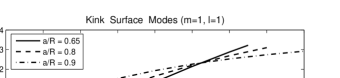
Figure 1: Frequency of the fundamental kink ($m=1$) surface mode and its damping rate versus the twist parameter, $B_{\phi}/B_{z}$, for different relative core width $a/R=$ 0.65 (solid), 0.8 (dashed) and 0.9 (dash-dotted). The loop parameters are: $L=109\times 10^{3}$ km, $R/L=0.01$, $\rho_{e}/\rho_{i}=0.1$, $\rho_{0}/\rho_{i}=0.5$, $\rho_{i}=2\times 10^{-14}$ gr cm^-3, $B_{e}/B_{i}=1$, $B_{0}/B_{i}=1$, $B_{i}=100$ G, $S=10^{4}$ and ${\mathcal{R}}=560$. Both frequencies and damping rates are in units of the interior Alfvén frequency, $\omega_{\rm A_{i}}=1.835{\rm~{}rad~{}s^{-1}}$.

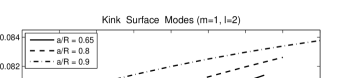
Figure 2: Same as Fig. 1, for the first-overtone kink ($m=1$) surface modes.

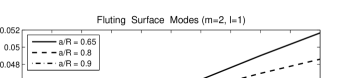
Figure 3: Same as Fig. 1, for the fundamental fluting ($m=2$) surface modes.

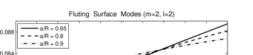
Figure 4: Same as Fig. 1, for the first-overtone fluting ($m=2$) surface modes.

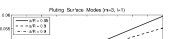
Figure 5: Same as Fig. 1, for the fundamental fluting ($m=3$) surface modes.

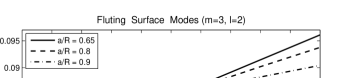
Figure 6: Same as Fig. 1, for the first-overtone fluting ($m=3$) surface modes.

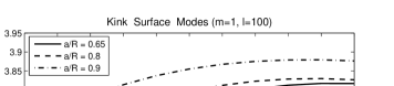
Figure 7: Same as Fig. 1, for the kink ($m=1$) surface modes with $l=100$.

Figure 8: The period ratio $P_{1}/2P_{2}$ of the fundamental and its first-overtone kink ($m=1$) surface modes versus the twist parameter for different relative core width $a/R=$ 0.65 (solid), 0.8 (dashed) and 0.9 (dash-dotted). Auxiliary parameters as in Fig. 1.

Figure 9: Same as Fig. 8, for fluting ($m=2$) surface modes.

Figure 10: Same as Fig. 8, for fluting ($m=3$) surface modes.

Figure 11: Frequency band width of the fundamental kink ($m=1$) hybrid modes versus the twist parameter for different relative core width $a/R=$ 0.65 (solid), 0.8 (dashed) and 0.9 (dash-dotted). Auxiliary parameters as in Fig. 1.

References

- [1] Andries J., Goossens M., Hollweg J.V., Arregui I., Van Doorsselaere T., 2005, A&A, 430, 1109
- [2] Aschwanden M.J., 2005, Physics of the Solar Corona. Springer, Berlin, p. 305
- [3] Aschwanden M.J., Fletcher L., Schrijver C.J., Alexander D., 1999, ApJ, 520, 880
- [4] Bennett K., Roberts B., Narain U., 1999, Sol. Phys., 185, 41
- [5] Carter B. K., Erdélyi R., 2007, A&A, 475, 323
- [6] Carter B. K., Erdélyi R., 2008, A&A, 481, 239
- [7] De Pontieu B., Martens P.C.H., Hudson H.S., 2001, ApJ, 558, 859
- [8] Edwin P.M., Roberts B., 1983, Sol. Phys., 88, 179
- [9] Erdélyi R., Carter B.K., 2006, A&A, 455, 361
- [10] Erdélyi R., Fedun V., 2006, Sol. Phys., 238, 41
- [11] Erdélyi R., Verth G., 2007, A&A, 462, 743
- [12] Karami K., Asvar A., 2007, MNRAS, 381, 97
- [13] Karami K., Nasiri S., Sobouti Y., 2002, A&A, 396, 993
- [14] Klimchuk J. A., Antiochos S.K., Norton D., 2000, ApJ, 542, 504
- [15] McEwan M.P., Díaz A.J., Roberts B., 2008, A&A, 481, 819
- [16] Mikhalyaev B.B., Solov’ev A.A., 2005, Sol. Phys., 227, 249
- [17] Nakariakov V.M., Ofman L., DeLuca E.E., Roberts B., Davila J.M., 1999, Science, 285, 862
- [18] Ofman L., Davila J.M., Steinolfson R.S., 1994, ApJ, 421, 360
- [19] Steinolfson R.S., Davila J.M., 1993, ApJ, 415, 354
- [20] Van Doorsselaere T., Debosscher A., Andries J., Poedts S., 2004, A&A, 424, 1065
- [21] Verwichte E., Nakariakov V. M., Ofman L., Deluca E. E., 2004, Sol. Phys., 223,77
- [22] Wang T.J., Solanki S.K., 2004, A&A, 421, L33