The Antares emission nebula and mass loss of $\alpha$ Sco A

Abstract

Aims. The Antares nebula is a peculiar emission nebula seen in numerous [Fe ii] lines and in radio free-free emission, probably associated with the H ii region caused by $\alpha$ Sco B in the wind of $\alpha$ Sco A. High-resolution spectra with spatial resolution were used to study the emission line spectrum, the physical nature of the nebula and to determine the mass-loss rate of the M supergiant $\alpha$ Sco A.

Methods. The Antares nebula was mapped with long-slit (10$\arcsec$) and high-resolution ($R=80\,000$) spectra using UVES at the VLT. The resulting 2-D images were used to reconstruct a 3-D picture of the H ii region and its absolute location in space relative to $\alpha$ Sco A.

Results. We found that the Antares nebula shows, in addition to numerous [Fe ii] lines, the Balmer line recombination spectrum H_α, H_β up to H₁₀, and [N ii] 6583/6548 Å, H_α and [N ii] with the same extent as seen in cm radio free-free emission. Combining velocity information from optical and GHRS/HST spectra with H_α velocities, the H ii region is found to be located $\sim 215$ AU behind the plane of the sky of $\alpha$ Sco A. From the H_α/[N ii] intensity ratio and the non-visibility of the [O ii] 3726/3729 Å lines we estimate a low mean electron temperature of $\overline{T}_{\rm e}=4900$ K and an N abundance enhanced by a factor of $\sim$ 3 due to the CNO cycle in $\alpha$ Sco A. The shape and size of the H ii region yield a mean mass-loss rate of (1.05 $\pm$ 0.3) $\times$ 10^-6 M_⊙ yr^-1. The [Fe ii] lines originate predominantly at the edges (rear and front) of the H ii region. UV continuum pumping as well as collisional excitation seem to be responsible for the observed iron lines.

1 Introduction

The Antares nebula is a unique object in the sky. Antares ($\alpha$ Sco A, M 1.5 Iab) and its blue visual companion $\alpha$ Sco B (B 2.5 V) are known to be surrounded by a circumstellar envelope seen in absorption in both components which can be used to determine the mass-loss rate of the M supergiant (Deutsch deu60 (1960); Kudritzki & Reimers kud78 (1978); Hagen et al. hag87 (1987); Baade & Reimers baa07 (2007)). The common envelope has also been known for a long time as an emission nebula with strong [Fe ii] lines (Wilson & Sanford wil37 (1937); Struve & Swings str40 (1940); Swings & Preston swi78 (1978)). The most extensive study was that by Swings & Preston (swi78 (1978)) based on high-resolution long-slit photographic Coudé spectra taken with the Mount Wilson 100 inch and Palomar 200 inch telescopes. They found that the “[Fe ii]-rich nebula” is strong roughly $3\aas@@fstack{\prime\prime}5$ around the B star surrounded by a zone of weaker lines which may extend in the NW-SE direction up to $15\arcsec$. It has been shown by Kudritzki & Reimers (kud78 (1978)) that the [Fe ii] emission lines are probably associated with the H ii region formed by the B star within the stellar wind of the M supergiant.

The H ii region has been detected and resolved at cm radio wavelengths with the VLA (Hjellming & Newell hje83 (1983)). The maximum H ii region radio emission was found to be centered roughly $0\aas@@fstack{\prime\prime}5$ from the B star on the line connecting the two stars.

Several questions remained unanswered. Why are the Balmer lines, expected in emission due to recombination within the H ii region, absent or weak compared to the [Fe ii] lines? Why are the “classical” H ii region emission lines absent or weak? Why are the [Fe ii] lines double west of B, but single east of B (between the two stars)? With the advent of UVES at the VLT it was obvious that progress in our understanding of the kinematics of the Antares nebula is now possible due to the high spectral resolution, high pointing accuracy, and stability of UVES. We used the spectrograph at a resolution of 80 000 to map the nebula in 2-D with 23 slit positions covering the whole nebula (Fig. 1).

In section 2 we describe the observations and the data reduction which was difficult due to (unexpected) scattered light from the M supergiant even 10$\arcsec$ away from the bright star. Section 3 gives a phenomenological description of the observations. In section 4 we present the analysis of the UVES spectra as well as a discussion of the obtained results.

2 Observations and data reduction

2.1 Observations

The observations were performed with the UVES spectrograph at the VLT/ESO (Dekker et al. dek00 (2000)) in service mode. To cover the spectral range from $\sim 3050$ to 11 000 Å two pairs of standard settings of the double-spectrograph were used: one with a central wavelength of 3460 Å for the blue arm covering the range from $\sim 3050$ to 3850 Å and simultaneously for the red arm with a central wavelength of 5800 Å covering the range from 4200 to 6800 Å with an exposure time of 100 s and the other with an exposure time of 50 s at a central wavelength of 3900 Å for the range from 3750 to 5100 Å in the blue and at 8600 Å for the range from 6600 to 11 000 Å in the red. The slit size in the blue arm was $0\aas@@fstack{\prime\prime}4\times 10\arcsec$ and $0\aas@@fstack{\prime\prime}4\times 12\arcsec$ in the red. We chose 23 different pointings for both setting pairs to cover the main part of the nebula in the sky (cf. Fig. 1). The 45° positions were observed on September 29, 2005, the inner 10 ones on February 17, 2006, and the remaining most westward positions on February 16, 2006. The typical seeing was $0\aas@@fstack{\prime\prime}6$, slightly larger than the slit separations.

Figure 1: Geometry of the Antares system together with true spectrograph slit sizes and positions projected to scale on the sky. The slit length is $10\arcsec$ referring to the blue arm. Slit positions are $0\aas@@fstack{\prime\prime}9$, $1\aas@@fstack{\prime\prime}4$. in steps of $0\aas@@fstack{\prime\prime}5$ (cf Fig. 2) relative to the M star, perpendicular to the line A-B. Two slit positions are tilted by 45° as displayed.

2.2 Data reduction

The position of the echelle orders were determined by searching for the exposed areas of the flat field exposures and corresponding masks were used for further data reduction. The flat-field corrected science data were aligned parallel to the order boundaries and calibrated with Th-Ar comparison exposures resulting in two-dimensional rectangular data arrays for each order with one axis representing the wavelength, the other the position along the slit.

Unexpectedly, all spectra – even $10\arcsec$ from the M supergiant – are completely corrupted by scattered light from the M star. This was a surprise also for the UVES team at ESO. ESO finally performed a test with the UVES slit $10\arcsec$ apart east and west of a bright star - with the same result as in our spectra. Apparently, light from the bright star is scattered by the slit jaws back to the slit viewing camera and from there again into the spectrograph slit. The UVES team comment: “Our conclusion is that one should not trust any light excess in the reconstructed image, since these are most likely due to reflexions caused by the bright star, as it is the case in the test.”

Due to the ubiquitous scattered light, no general background reduction was possible. For each spectral line a local background had to be determined. Due to the lack of a pure spectrum of $\alpha$ Sco A the central region of the data at the first slit position – where the scattered light of the M star is brightest and therefore the ratio of the nebula emission to the M star light is smallest – was used as a background template. The template was fitted to the data allowing a scale and an offset. A region of +/- 30 km s^-1 around the laboratory wavelength of the spectral line was excluded while fitting. This background was subtracted from the data. For slit positions near the B-star additional scattered light was present. This could be reduced using a square spline fit to the remaining continuum.

As a further consequence of the heavy contamination of the nebula spectrum with M star light – the nebula spectrum is always faint compared to the scattered light spectrum – we are not able to provide quantitative line fluxes, except for relative fluxes of neighboring lines.

Table 1: Antares nebula emission lines

$\lambda$  [Å]	ion		$\lambda$  [Å]	ion
3076.07	[Ni ii]		4276.83	[Fe ii]
3175.38	[Fe ii]		4287.40	[Fe ii]
3177.53	Fe ii		4305.90	[Fe ii]
3186.74	Fe ii		4319.62	[Fe ii]
3192.91	Fe ii		4326.24	[Ni ii]
3193.43			4340.47	H$\gamma$
3193.80	Fe ii		4346.85	[Fe ii]
3196.07	Fe ii		4352.78	[Fe ii]
3210.04	Fe ii		4358.37	[Fe ii]
3213.31	Fe ii		4359.34	[Fe ii]
3214.67	Fe ii		4372.43	[Fe ii]
3223.15	[Ni ii]		4382.75	[Fe ii]
3227.74	Fe ii		4413.78	[Fe ii]
3255.89	Fe ii		4416.27	[Fe ii]
3277.55	[Fe ii]		4452.11	[Fe ii]
3376.20	[Fe ii]		4457.95	[Fe ii]
3378.16	[Ni ii]		4474.91	[Fe ii]
3387.09	[Fe ii]		4488.75	[Fe ii]
3438.89	[Ni ii]		4492.64	[Fe ii]
3441.00	[Fe ii]		4514.90	[Fe ii]
3442.04			4728.07	[Fe ii]
3452.31	[Fe ii]		4774.74	[Fe ii]
3455.11	[Fe ii]		4814.55	[Fe ii]
3501.63	[Fe ii]		4861.33	H$\beta$
3504.02	[Fe ii]		4874.49	[Fe ii]
3504.51	[Fe ii]		4889.63	[Fe ii]
3514.05			4905.35	[Fe ii]
3538.69	[Fe ii]		4923.92	Fe ii
3539.19	[Fe ii]		5018.44	Fe ii
3559.41	[Ni ii]		5041.03	Si ii
3626.89	[Ni ii]		5055.98	Si ii
3856.02	Si ii		5056.32	Si ii
3862.59	Si ii		5111.63	[Fe ii]
3970.07	H$\epsilon$		5158.78	[Fe ii]
3993.06	[Ni ii]		5163.95	Fe ii
4101.74	H$\delta$		5169.03	Fe ii
4114.48	[Fe ii]		5261.62	[Fe ii]
4147.26	Fe ii		5273.35	[Fe ii]
4177.21	[Fe ii]		5333.65	[Fe ii]
4178.95	[Fe ii]		6347.11	Si ii
4211.10	[Fe ii]		6371.37	Si ii
4243.98	[Fe ii]		6548.05	[N ii]
4244.81	[Fe ii]		6562.85	H$\alpha$
4248.83			6583.45	[N ii]
4251.44	[Fe ii]?		7377.83	[Ni ii]

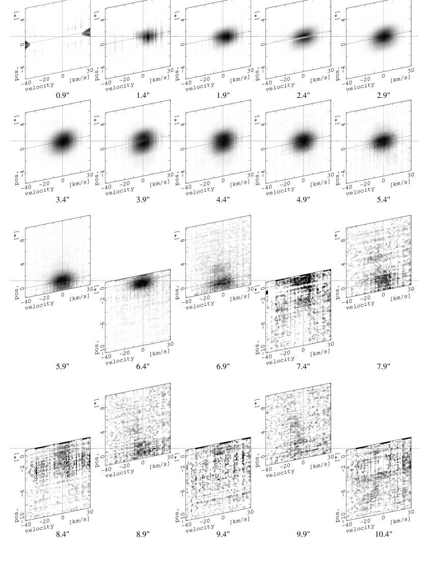
Figure 2: H_α 2-D brightness distributions as a function of the spectrograph slit position relative to $\alpha$ Sco A as shown in Fig 1. Notice that due to the M star wind expansion, the velocity coordinate corresponds to the spatial depth (perpendicular to the plane of the sky). The density in the plots has been rescaled in order to provide maximum visibility. The total counts vary by a factor of $\sim 150$ between $1\aas@@fstack{\prime\prime}9$ and $8\aas@@fstack{\prime\prime}9$.

Figure 3: Comparison of the distribution of H_α emission (dashed) with radio free-free emission (full lines) (Hjellming & Newell hje83 (1983)). Dashed lines represent half, fourth, and tenth contour levels of the central emission flux.

3 Phenomenological description of the observations

3.1 The emission line spectrum

A list of emission lines in the spectral range 3050 to 7400 Å is given in Table 1. Compared to the line list of Swings & Preston (swi78 (1978)) we cover a larger wavelength range with many new lines below 3225 Å and longward of 4500 Å. In addition, the higher spectral resolution combined with a digital detector (compared to Swings & Preston’s photographic spectra) allowed a better subtraction of the contaminating M star light which led to the removal of some of the lines given by Swings & Preston, e.g. 3427, 3991, 4018, 4088, 4127, 4178, 4233, 4423, 4471, and 4483 Å. Most of them had been classified already as doubtful by these authors. Altogether the number of unambiguously detected emission lines has been more than doubled. Identifications were made using the NBS online data bank NIST (Ralchenko et al. ral07 (2007)).

For the physical interpretation of the nebula, the detection of H_α to H₁₀ is important, since the recombination lines can be used to map the geometrical extent of the H ii region for a comparison with a radio map and to locate the H ii region in velocity space which should allow us to determine its position relative to the plane of the sky.

We confirm that the strongest lines are the forbidden iron lines [Fe ii] 4287, 4359, 4416, 4414, and 4814 Å. We have also detected a number of allowed Fe ii lines. The Fe ii mult. 42 lines 5169, 5018, and 4924 Å which feed the upper level of the strongest forbidden [Fe ii] lines 4287 and 4359 Å are noticable. The mult. 42 lines are obviously produced by UV pumping via the strong resonance scattering line of the UV mult. 3 at 2343 Å seen in UV spectra of $\alpha$ Sco B (Hagen et al. hag87 (1987)).

Figure 4: [Fe ii] 4814.55 Å 2-D brightness distributions as a function of the spectrograph slit position (see notes in caption of Fig. 2).

3.2 The spatial extent and velocity field in the Antares nebula

After having carefully subtracted the underlying continua of scattered light, the mapping of the nebula by long-slit spectroscopy in steps of 0$\aas@@fstack{\prime\prime}$5 in the E-W direction allows us to construct 2-D images (space versus velocity) of the emission nebula, in particular in the strongest lines as a function of the slit position. In the following we discuss the velocity-space images separately for different types of lines.

3.2.1 Balmer lines

Previous work (Kudritzki & Reimers kud78 (1978); Hjellming & Newell hje83 (1983)) has shown that the hot B star creates an H ii region within the wind of the M supergiant. The extent of the H ii region (ionization bounded or not) depends on the mass-loss rate of the supergiant and on the number of Lyman continuum photons of $\alpha$ Sco B. The H ii region was seen in free-free radio emission and its recombination spectrum should show Balmer lines in emission.

Swings & Preston (swi78 (1978)) did not see H_β and H_γ emission lines in their photographic spectra. Fig. 2 shows that H_α emission has an extent along the slit of $\sim 4\arcsec$, nearly independent of the slit position, except the position closest to the M star ($1\aas@@fstack{\prime\prime}4$ from the M giant) where the emission region appears narrower ($\sim 3\arcsec$). At position $0\aas@@fstack{\prime\prime}9$ from the M star there is no H_α emission. In velocity space the center of the H_α emission is always positive relative to the M star velocity, indicating that the B star is located beyond the plane of the M star (see below) in agreement with Baade & Reimers (baa07 (2007)).

A comparison of the extent of radio free-free emission observed with the VLA (Hjellming & Newell hje83 (1983)) with the extent of H_α emission measured from the data displayed in Fig. 3 shows that around the B star and in the direction of the M supergiant the location of H_α, H_β, and radio free-free emission is identical within the resolution. West of B, H_α is more extended, since it can be seen up to $4\arcsec$ in this direction. Apparently, the Balmer lines are a more sensitive probe of the H ii region. The Balmer line series can be seen up to H₁₀.

Table 2: Comparison of line strengths of H_α and [N ii] 6583.45 Å for slit positions in the H ii region.

distance to M star [″]	Hα/[N ii]
1.4	$2.7\pm 0.9$
1.9	$3.9\pm 1.7$
2.4	$3.7\pm 1.6$
2.9	$3.3\pm 1.0$
3.4	$3.8\pm 1.0$
3.9	$4.5\pm 1.3$
4.4	$5.8\pm 1.9$
4.9	$8.0\pm 1.8$
5.4	$10.3\pm 5.4$
5.9	$7.7\pm 3.3$
6.4	$11.5\pm 6.5$
6.9	$9.5\pm 10.7$

3.2.2 [N ii] emission

In all previous investigations of the Antares nebula the question remained open, why the “classical” emission lines, normally prominent in H ii region spectra, like [O iii] 4959/5007 Å, [O ii] 3726/3729 Å, [N ii] 6583/6548 Å, and [S ii] 6716/6731 Å, were not detected. Our UVES spectra allow a more critical assessment than earlier photographic spectra like those used e.g. by Swings & Preston (swi78 (1978)). In addition we have 10 long-slit positions covering the H ii region (cf. Fig. 1) which gave us the possibility of detecting faint H ii emission lines. The result is that except for [N ii] 6583 Å and 6548 Å none of the H ii region lines, in particular [O ii] 3726/3729 Å or [O i] 6300/6363 Å, were detected. [N ii] 6583 Å closely follows the H_α distribution shown in Fig. 2. Since it lies close to the H_α line, we can measure the H_α/[N ii] ratio as a function of the location in the nebula (Table 2).

Figure 5: [Fe ii] 4814.55 Å 2-D brightness distribution at the 45° NE slit position, logarithmically scaled.

3.2.3 The allowed lines

The Si ii lines 6347, 6371, 3862, and 3856 Å roughly follow the H_α distribution (Fig. 2) in that the emission does not extend beyond 1$\aas@@fstack{\prime\prime}$5 east of B. In velocity space they are narrower (0 to +10 km s^-1) than the H_α distribution. The reason cannot be the smaller thermal broadening of Si ii lines compared to H_α, since at 5000 K the thermal width is $\sim 1\,{\rm km\,s^{-1}}$, small compared to the much larger wind microturbulence that is typically half the wind velocity. The simplest interpretation would be that the Si ii lines are formed close to the B star by Si iii recombination in a narrower velocity space (wind sector) than H_α. Unfortunately we have no Si iii 1206 Å absorption data. However, the existence and velocity of Al iii absorption lines do show that they must be formed in the immediate surroundings of the B star (Baade & Reimers baa07 (2007)). The narrowness of the Si iii region is confirmed by our final H ii region model.

The strongest allowed line is Fe ii 3228 Å. Its distribution is similar to that of the [Fe ii] lines and distinctly different from Si ii. It is clearly present 0$\aas@@fstack{\prime\prime}$9 from the M supergiant, i.e. outside the H ii region. The most interesting allowed Fe ii line is 5169 Å, since the appearance of this line both in the neutral wind (position 0$\aas@@fstack{\prime\prime}$9 from the M star) and in the H ii region indicates that one channel for the excitation of the forbidden [Fe ii] lines is line scattering of B star photons in the strong UV Fe ii resonance lines. One of the strong UV resonance lines in the UV spectrum of $\alpha$ Sco B is the UV mult. 3 line at 2343 Å. These lines show P Cyg type profiles (cf. Hagen et al. hag87 (1987)). In case of the 2343 Å line a second downward channel exists via the Fe ii lines 4924, 5018, and 5169 Å. The branching ratio of the 2343 Å and 4924 - 5169 Å lines is $\sim 16$ (NIST-data base, Ralchenko et al. ral07 (2007)), so that part of the downward cascade is via the three 4923 - 5169 Å lines and this is what we observe. In the neutral wind we can detect both the 2343 Å reemission part of the P Cyg profile and the 4924 - 5169 Å channel in emission which populates the upper level of the strongest [Fe ii] lines 4287 Å and 4359 Å.

Figure 6: [Fe ii] 4814.55 Å 2-D brightness distributions of Fig. 4 transformed to spatial coordinates using an M star wind velocity of 20 km s^-1.

In conclusion: We have directly identified the [Fe ii] excitation mechanism in the cold neutral M supergiant wind, i.e. the faint extended emission region outside the H ii region which is marked by H_α emission, radio free-free emission, and Si ii emission. This Fe ii resonance line scattering mechanism is certainly also operating in the H ii region, but the comparison of the distribution of the strong [Fe ii] lines with Fe ii 5169 Å shows that within the H ii region either other excitation mechanisms are dominant, e.g. collisional excitation by free electrons in the H ii region, or iron is more abundant in the gas phase.

3.2.4 [Fe ii] emission

In the most extensive study of the emission spectrum of the Antares nebula by Swings & Preston (swi78 (1978)), the “[Fe ii] rich” nebula was described as an asymmetrical region of about 3$\aas@@fstack{\prime\prime}$5 around the B star with strong lines, surrounded by a much more extended region of weaker lines. Our data, shown in Fig. 4, are largely consistent with Swings & Preston (swi78 (1978)) but give a more detailed picture due to the higher spectral resolution (80 000) and angular resolution, since most of the data were taken at 0$\aas@@fstack{\prime\prime}$6 seeing. This means that the resolution corresponds roughly to the slit steps (Fig. 1). Below we summarize the main characteristics:

• We notice in particular that [Fe ii] emission is apparently concentrated on the ionization front in a cone-like structure. This can be seen clearly in Fig. 4 at slit positions 2$\aas@@fstack{\prime\prime}$9, 3$\aas@@fstack{\prime\prime}$4, 5$\aas@@fstack{\prime\prime}$9, and 6$\aas@@fstack{\prime\prime}$9. The reason for the [Fe ii] enhancement at the H ii/H i interface may be shock heating. Since the pressure in the H ii region is higher by a factor of $\sim 10$ than in the cool wind, a shock front will build up at the interface (cf. Kudritzki & Reimers kud78 (1978)). The occurrence of [Fe ii] in the Orion Nebula has also been observed close to the ionization front (Bautista et al. bau94 (1994)).

• Contrary to the nondetection in H_α, [Fe ii] is already seen 0$\aas@@fstack{\prime\prime}$9 from the M supergiant. This is a consequence of the origin of these lines that are produced via pumping processes as described in section 3.2.3 and 4.5.

• It is obvious that beyond $\sim 5\aas@@fstack{\prime\prime}$9 west of A, the [Fe ii] emission, although weak, becomes more extended and structured (“cloudy”).

  West of B and increasing with distance from B the lines appear as double and triple. The double lines were already reported by Deutsch (deu60 (1960)) and Struve & Zebergs (str62 (1962)).

  Both of the 45° positions with slit length 12$\arcsec$ starting from B (Fig. 5) show that the emission maximum is not close to B but $\sim 1\arcsec$ apart. Furthermore, weak [Fe ii] emission is seen all along the slit, confirming Swings & Preston (swi78 (1978)) who saw [Fe ii] up to 15$\arcsec$ in the SE direction.

• It can also be seen from Fig. 4 that in the emission line region the median in velocities moves systematically from $\sim 4$ km s^-1 1$\aas@@fstack{\prime\prime}$9 west of A over 3 km s^-1 at B to 0 km s^-1 5$\aas@@fstack{\prime\prime}$9 west of A and -5 km s^-1 at 9$\aas@@fstack{\prime\prime}$9 west of A.

• The nebula shows large scale deviations from a simple geometry like a smooth spherically expanding M star wind in which the B star produces an ellipsoid-like H ii region. In reality the [Fe ii] emitting regions have a clumpy structure with discrete “blobs”. This is in accordance with the shell structure seen in the IR (Marsh et al. mar01 (2001)) and the episodic mass loss seen in UV resonance lines (Baade & Reimers baa07 (2007)).

4 Analysis and discussion

4.1 The location of B relative to the plane of the sky

The velocity of the circumstellar Ti ii absorption lines in the line of sight had been used together with the assumption of a spherical wind with a constant expansion velocity to estimate a position of B $\sim 600$ AU in front of the plane of the sky (Kudritzki & Reimers kud78 (1978)). However, the observed episodic nature of mass loss of $\alpha$ Sco A (4 absorption components) disagrees with these assumptions and the derived location must be considered as erroneous (Baade & Reimers baa07 (2007)).

GHRS/HST spectra show that the Al iii absorption lines at +7.8 km s^-1, which must be formed close to the B star, favor a location of B roughly 224 AU behind the M star (Baade & Reimers baa07 (2007)). We can determine the B star position independently using the velocity of the H_α line at the eastern boundary of the H ii region at the slit positions 1$\aas@@fstack{\prime\prime}$4 and 1$\aas@@fstack{\prime\prime}$9. The basic underlying assumption is that the M star wind velocity is not severely disturbed and that the width of the emission defines the front and rear side of the H ii region. The mean observed velocity in the line of sight is $\sim 4.8$ km s^-1, i.e. 7.8 km s^-1 relative to the M supergiant. Using a constant M star wind velocity of 20 km s^-1 (Baade & Reimers baa07 (2007)), we obtain a position angle of 23^∘ behind the M star with an uncertainty of about 5^∘. A measurement of the [Fe ii] lines of the H i region in front of the H ii region, where the lines are formed by UV pumping, gives a nearly identical result.

4.2 Geometry and binary orbit

Long-term observations of the visual binary have shown that the orbit is nearly in the line of sight (Hopmann hop57 (1957)), and the binary separation has become smaller from 3$\aas@@fstack{\prime\prime}$01 in 1930 (photographic plates, Hopmann hop57 (1957)) to 2$\aas@@fstack{\prime\prime}$86 in 1989 (interferometric measurements, McAlister et al. mca90 (1990)), and to 2$\aas@@fstack{\prime\prime}$74 in 2005 (lunar occultation, Sôma som06 (2006)). The extrapolation yields a separation of 2$\aas@@fstack{\prime\prime}$73 in February 2006. With the Hipparcos distance of 185 pc and assuming a circular orbit we obtain a semi-major axis of 549 AU. With 18 M_⊙ and 7.2 M_⊙ for $\alpha$ Sco A and B, respectively (Kudritzki & Reimers kud78 (1978)), Kepler’s third law yields a binary period of 2562 yrs. The corresponding calculated orbital velocities are $v_{\rm M}=-1.82\,\rm km\,s^{-1}$ and $v_{\rm B}=4.56\,\rm km\,s^{-1}$, with radial components $v_{\rm M,r}=-1.68\,\rm km\,s^{-1}$ and $v_{\rm B,r}=4.20\,\rm km\,s^{-1}$. This is close to the observed values of -3 km s^-1 and +3 km s^-1 for the M and B star, respectively (Evans eva67 (1967); Kudritzki & Reimers kud78 (1978)), if a small systemic velocity of -1.25 km s^-1 is added. Unfortunately the observational data do not allow us to establish a reliable orbital solution. If we trust the 19th century measurements compiled by Hopmann (hop57 (1957)) the orbit cannot be circular. However, for the present work the uncertainties of the binary orbit can be neglected.

4.3 The shape of the H ii region

The apparent shape of the H_α emission nebula in the sky according to Fig. 2 is displayed in Fig. 3, together with the radio map of Hjellming & Newell (hje83 (1983)). Details of the H_α and [Fe ii] intensity projected onto the plane of the sky (2-D) have been presented in the sections 3.2.1 and 3.2.4. The emission nebula can be best described by a bow-shock shaped region with its front $\sim 1\arcsec$ east of B which opens slowly to an extent of roughly 6$\arcsec$ up to $\sim 3\arcsec$ west of B. Beyond 3$\arcsec$ the “shock cone” opens with filamentary structures to an extent of up to nearly 16$\arcsec$ ($\pm$ 8$\arcsec$). In velocity space the “double line” character becomes more distinct, and typically the red line edge is sharply limited. We appear to look through a shock cone with a front and rear edge (cf. Fig. 4 on and slightly west of B).

With the assumption that the M star wind continues at constant velocity through the H ii region without being grossly disturbed, we can construct a 3-D image of the [Fe ii] emitting gas since each velocity in Fig. 4 corresponds in that case to a location relative to the plane of the sky (positive velocities behind, negative velocities in front of the plane of the sky). The resulting 2-D slices for each slit position are presented in Fig. 6: East of B the emission comes from behind the plane of the sky, as expected, since the B star and the surrounding H ii region are behind the plane of the sky. Between the position of B and $\sim 3\arcsec$ west of B, the emission comes from a region of cylindrical shape with a diameter of $\sim 6\arcsec$. This extent is almost identical in the plane of the sky and in the vertical direction. A gradual apparent shift of the [Fe ii] emitting gas is seen from 200 AU behind the plane at 1$\aas@@fstack{\prime\prime}$4, slightly behind the plane of the sky (on average) to an extent of between 740 AU behind to 1480 AU in front of the plane of the sky. The shock cone apparently opens up beyond 3$\arcsec$ west of B to larger distances in front of the plane of the sky.

4.4 Where are the “normal” forbidden H ii region lines?

The Antares nebula has been considered as “peculiar” from its detection (cf. the extensive discussion in Struve & Zebergs str62 (1962)) because its spectrum is dominated by numerous strong [Fe ii] lines while the classical H ii region lines [O ii] 3287 Å, [O ii] 3726/3729 Å, [O iii] 4957/5007 Å, and [S ii] are missing. Only the [N ii] lines are present. Since $\alpha$ Sco B is with B 2.5 V of much later spectral class than the O stars normally exciting an H ii region, we expect a lower electron temperature. Swings & Preston (swi78 (1978)) had estimated $T_{\rm e}\approx 4000$ K from the [Fe ii] excitation, while Kudritzki & Reimers (kud78 (1978)) estimated $T_{\rm e}=4000$ K from the heating/cooling balance. The latter value , however, was based on normal H ii region cooling rates dominated by [O iii], [O ii] etc. and is not applicable according to the present work.

Figure 7: Theoretical run of the electron temperature in different directions as a function of distance from the B star. The CLOUDY models are presented for 11 equidistant angles in the H ii region between 0° and 180°, where 0° corresponds to the connecting line between the two stars. The density distribution used here and in Fig. 9 is $n\sim r^{-2}$ according to constant wind expansion from the M star.

Figure 8: “Look back” contours (solid lines) of H ii region borders in a plane perpendicular to the plane of the sky caused by the combination of wind expansion and orbital motion of $\alpha$ Sco B relative to $\alpha$ Sco A shown for present and previous phases (-120 yrs to -360 yrs; 130 years being the wind travel time for the projected distance between A and B). This can be interpreted as a qualitative model for the comet like structure of the [Fe ii] emission regions. For clarification we overlay the projected brightness distribution of Fig. 6.

The key to an understanding of the missing [O ii], [O iii] lines with the simultaneous presence of the [N ii] lines is twofold: electron temperature and abundance. At first, the electron temperature of the H ii region must be so low that for normal or slightly reduced O/H ratios [O ii] 3726/3729 Å must be below the detection limit. For [O ii] 3726/3729 Å we can give an upper limit: we have detected the Balmer line series up to H₁₀, H₁₁ (close to [O ii]) not being visible. Thus the H₁₀ intensity, as predicted by recombination theory, can be regarded as an upper limit to [O ii] which yields [O ii]/H${}_{\alpha}<$ 0.017 for 3726 Å. Models calculated for the Antares H ii region with the ionization code CLOUDY (version 07.02.00, last described by Ferland et al. fer98 (1998)) lead to $T_{\rm e}<5000$ K. At such a low $T_{\rm e}$, [N ii]/H_α would be $<0.1$ (see also Fig. 3 in Mierkewicz et al. mie06 (2006)) for solar abundances and thus below our detection limit, while the observed [N ii] 6583 Å/H_α is between 0.3 and 0.4 in the central region of the H ii region. The solution to this puzzle is that the atmospheric (and wind) composition of the M supergiant must have been altered by the CNO cycle.

When a star ascends the red giant branch the first dredge-up may alter the CNO abundance significantly. The exact amount of the depletion of O and enhancement of N depends on the initial mass. As a consequence it is difficult to derive exact CNO abundances for $\alpha$ Sco A on the basis of evolutionary tracks, since neither its current mass nor the mass it had on the main sequence are reliably known. Recently Balachandran et al. (bal06 (2006)) have published abundance measurements of a number of M type supergiants that suggest $\rm[N/O]\sim 0.7$ for $\alpha$ Sco A.

While the CNO abundance ratios have not been measured in $\alpha$ Sco A, Harris & Lambert (har84 (1984)) have found that ¹⁷O and ¹³C are enriched so that there is also clear observational evidence for CNO cycle material in the envelope of $\alpha$ Sco A. Our best model for the H ii region leads to $\rm N/N_{\odot}=3.3\pm 1$ and $\rm O/O_{\odot}\la 0.9\pm 0.1$, i.e $\rm[N/O]=0.56\pm 0.2$ which is consistent with the above-mentioned values for M supergiants. The final CLOUDY H ii region model used for Fig 7 and Fig 9 has solar abundances except for CNO for which we used the above numbers.

The nondetection of [S ii] 6716/6731 Å can be understood with the same arguments. In classical, relatively cool H ii regions, [S ii]/[N ii] is typically $\sim 0.3$ for solar abundances. With N being enhanced by a factor of more than 3, the expected [S ii]/[N ii] ratio is $<0.1$, consistent with the nondetection in our spectra.

The ionization structure and temperature of the H ii region depend primarily on the number of incident Lyman continuum photons emitted by the B star. The most reliable estimate of the Lyman continuum luminosity $L_{\rm Ly}$ comes from radio measurements of the H ii region by Hjellming & Newell (hje83 (1983)). It is possible to adjust the effective temperature of the B star until the measured radio flux is reproduced. These calculations have to be performed iteratively, since the electron temperature $T_{\rm e}$ of the H ii region is a priori unknown. Only the knowledge of $T_{\rm e}$ allows us to quantify the relation between the Lyman continuum luminosity and the radio flux. A final model that satisfies all observational constraints yields a mean electron temperature of 4900 K. A detailed plot of the temperature distribution in the H ii region is shown in Fig. 7. It should be noted that Fe ii has a considerable impact on the H ii region and its electron temperature. As a consequence we apply the CLOUDY code with the more accurate Fe ii model using 371 levels as described by Verner et al. (ver99 (1999)).

4.5 What excites the [Fe ii] lines?

The [Fe ii] lines have been observed in high-density regions such as the Orion Nebula (Bautista et al. bau94 (1994); Baldwin et al. bal00 (2000)) and it has been shown by multilevel collisional-radiative Fe ii models that under the Orion Nebula conditions (at $n_{\rm e}=10^{4}\,\rm cm^{-3}$ and $T_{\rm e}=10^{4}\,\rm K$) the optical [Fe ii] lines (4814, 4277 Å etc.) are due to UV continuum pumping, while the infrared [Fe ii] lines are produced by collisional excitation (Baldwin et al. bal96 (1996), Verner et al. ver00 (2000)). The strong [Fe ii] line at 4814 Å as presented in Fig. 4 is the result of a pumping route starting from level a⁴F which is excited to level x⁴F^o. The downward transition to b⁴F followed by a transition back to the a⁴F term finally produces the observed line. Details of this and other Fe ii pumping processes are discussed thoroughly by Verner et al. ver00 (2000) (see especially their Fig. 7 showing all relevant routes of the continuum pumping).

In the case of the $\alpha$ Sco wind we explicitly showed above that in the neutral, cool wind (H i region) the [Fe ii] lines are visible and are formed by UV pumping. So the question remains: Why is the contrast between H ii region and H i region (Figs. 2, 4) so strong? At first, the [Fe ii] lines are strongest at the interface between the H ii and the H i region. Part of the explanation for this behavior is the fact that the Fe iii zone around the B star nearly fills the H ii region (in contrast to the smaller Si iii zone). This may lead to the triple velocity structure in [Fe ii] clearly visible at position $5\aas@@fstack{\prime\prime}4$ and $5\aas@@fstack{\prime\prime}9$ (Fig. 4), where the central component comes from Fe iii recombination and the ‘edge’ components from close to the ionization front.

Figure 9: Comparison of the velocity-integrated H_α flux with CLOUDY simulations shown for a mass-loss rate of $1.05\times 10^{-6}$ M_⊙ yr^-1. Since we have no absolute fluxes, both the observed (solid line) and the theoretical fluxes (dashed line) are normalized.

Secondly, as has been shown by HST spectra, iron (and consequently Fe ii) is depleted onto dust by at least a factor of 10 in the M giant wind (Fig. 4 in Baade & Reimers baa07 (2007)). The combination of density enhancement and grain destruction in the shock heated zone might be a further reason for the apparent [Fe ii] line enhancement at the H ii/H i interface. A further argument against pure collisional excitation of the [Fe ii] lines within the H ii region is our observation that the density enhanced shock zone is visible outwards to at least 7$\arcsec$ west of B, far beyond the H ii region which extends to roughly 3$\arcsec$ only.

The density enhancements made visible through [Fe ii] emission are apparently carried outwards by the M supergiant wind far beyond the H ii region and remain visible although H ii has recombined. Notice in particular the bright rear side and the fainter front side of the shock cone. The wind travel time $t_{\rm w}$ for 550 AU is $\sim 130$ yrs, to be compared with the recombination time $t_{\rm rec}$ of roughly 18 yrs for a mass-loss rate of $10^{-6}$ M_⊙ yr^-1 at the western border of the H ii region ($\sim 3\arcsec$ or $\sim 550$ AU west of B). Though $t_{\rm rec}$ is short compared to the wind travel time, advection effects may explain the existence of weak H_α emission outwards to $\sim 6\arcsec$ west of B.

We have schematically sketched this behavior showing the combined effect of B star orbital motion and wind expansion on the movement of a “former” H ii region (as seen in Fe) relative to the M supergiant. The simple model (Fig. 8) reproduces the location of the front and the rear edge of former H ii region gas in velocity space. With increasing distance from the B star, the median velocity moves from $+$4 km s^-1 1$\arcsec$ E of B over $+$3 km s^-1 at B to 0 km s^-1 W of B and $-$5 km s^-1 at 7$\arcsec$ W of B, consistent with the – vertical to the plane of the sky – cometary shaped Fe ii emission region as a result of the wind-carried density enhancements of the H i/H ii region interface.

From the above discussion it is obvious that a quantitative explanation of the [Fe ii] emission requires substantial additional effort: In a final step a non-stationary hydrodynamical model of the H ii region moving with the B star through the M star wind has to be computed. In a second step this model will be the basis for a 3D-NLTE radiative transfer model of Fe ii including the B star with the UV photons which, as we have shown, is at least partly responsible for the excitation of the [Fe ii] lines. Such a model is beyond the scope of the present paper.

4.6 Mass-loss rate

To quantify the mass-loss outflow we proceeded in two steps. Following Nussbaumer & Vogel (nus87 (1983)) we calculated in a first step the shape of the H ii region as a function of the mass-loss rate assuming an electron temperature of 4000 K (Kudritzki & Reimers kud78 (1978)) which is considered to be constant throughout the envelope. The resulting theoretical H ii region was projected onto the plane of the sky and compared to the observed H_α emission along the slits. Thus we obtained a tentative mass-loss rate of $8\times 10^{-7}$ M_⊙ yr^-1 that was used as the initial value for the subsequent step. In order to achieve a self-consistent model we used the ionization code CLOUDY (Ferland et al. fer98 (1998)) and constructed a static H ii region considering all relevant heating and cooling processes. The resulting temperature distribution is shown in Fig. 7. Now a more elaborate estimate of the mass-loss rate is possible using the spatially dependent emissivity. The emergent intensity of the H_α emission has been integrated for all slit positions as a function of the perpendicular distance from the central line. The best match with the observed intensity distribution yields mass-loss rates between $8.4\times 10^{-7}$ M_⊙ yr^-1 and $1.26\times 10^{-6}$ M_⊙ yr^-1. Fig. 9 shows the result for the mean value. There is a clear tendency that the required mass-loss rate increases for the outer slit positions. It is, however, questionable whether this finding reflects a true change in the mass outflow or is only an artifact of inhomogeneities or curved wind trajectories. It should be noted that the first slit position covers only part of the H ii region, resulting in a reduced emission.

We are aware that the static results of the CLOUDY code should be interpreted with care, but for optically thin media a correct implementation of the microphysics is more important than kinematic effects. Future work should include dynamical and time-dependent processes. Especially advection terms and hydrodynamical effects have to be considered carefully. Some of the observed features are clearly beyond the capabilities of a stationary model, as discussed above.

References

- (1) Baade, R., & Reimers, D. 2007, A&A 474, 229
- (2) Balachandran, S. C., Carr, J. S., & Venn, K. A. 2006, Mixing and CNO Abundances in M Supergiants. In: Chemical Abundances and Mixing in Stars in the Milky Way and its Satellites, ESO ASTROPHYSICS SYMPOSIA, Springer-Verlag, p. 204
- (3) Baldwin, J. A., Crotts, A., Dufour, R. J., Ferland, G., Heathcote, S. et al. 1996, ApJ 468, L115
- (4) Baldwin, J. A., Verner, E. M., Verner, D. A., Ferland, G. J., Martin, P. G., Korista, K. T., & Rubin, R. H. 2000, ApJS 129, 229
- (5) Bautista, M. A., Pradhan, A. K., & Osterbrock, D. E. 1994, ApJ 432, L135
- (6) Dekker, H. et al. 2000, SPIE, 4008, 534
- (7) Deutsch, A. 1960 in Struve and Zebergs,e.c. p. 303
- (8) Evans, D. S. 1967, IAUS 30, 57
- (9) Ferland, G. J., Korista, K. T., Verner, D. A., Ferguson, J. W., Kingdon, J. B., & Verner, E. M. 1998, PASP 110, 761
- (10) Hagen, H.-J., Hempe, K., & Reimers, D. 1987, A&A 184, 256
- (11) Harris, M. J., & Lambert, D. L. 1984, ApJ 281 739
- (12) Hjellming, R. M., & Newell, R. T. 1983, ApJ 275, 704
- (13) Hopmann, J. 1957, Mitt. Univers.-Sternwarte Wien, 9, 135
- (14) Kudritzki, R., & Reimers, D. 1978, A&A 70, 227
- (15) McAlister, H. A., Hartkopf, W. I., & Franz, O. G. 1990, AJ 99, 965
- (16) Marsh, K. A., Bloemhof, E. E., & Koerner, D. W., Ressler, M. E. 2001, ApJ 548, 861
- (17) Mierkiewicz, E. J., Reynolds, R. J., Roesler, F. L., Harlander, J. M., & Jachnig, K. P. 2006, ApJ 650, L63
- (18) Nussbaumer, H., & Vogel, M. 1987, A&A 182, 51
- (19) Osterbrock, D. E. 1989
- (20) Ralchenko, Yu., Jou, F.-C., Kelleher, D. E., Kramida, A. E., Musgrove, A., Reader, J., Wiese, W. L., & Olsen, K. 2007, NIST Atomic Spectra Database (version 3.1.2), [Online]. Available: http://physics.nist.gov/asd3 [2007, June 25]. National Institute of Standards and Technology, Gaithersburg, MD.
- (21) Sigut, T. A. A., & Pradhan, A. K. 2003, ApJS 145, 15
- (22) Sôma, M. 2006, Results from the Recent Lunar Occultations of upsilon Geminorum and Antares. In: A. Brzeziński, N. Capitaine, & B. Kołaczek (eds.) Journées 2005: Systèmes de Référence Spatio-Temporels (Earth dynamics and reference systems: five years after the adoption of the IAU 2000 Resolutions), p. 83
- (23) Struve, O., & Swings, P. 1940, ApJ 92, 316
- (24) Struve, O., & Zebergs, V. 1962, Astronomy of the 20th Century, MacMillan Comp. New York, p. 303ff
- (25) Swings, J. P., & Preston, G. W. 1978, ApJ 220, 883
- (26) Tsuji, T. 1985, ASSL 114, 295
- (27) Verner, E. M., Verner, D. A., Korista, K. T., Ferguson, J. W., Hamann, F., & Ferland, G. J. 1999, ApJS 120, 101
- (28) Verner, E. M., Verner, D. A., Baldwin, J. A., Ferland, G. J., & Martin, P. G. 2000, ApJ 543, 831
- (29) Wilson, O.C., & Sanford, R. F. 1937, PASP 49, 221